


Abstract
We present visible multi-band photometry of trans-Neptunian objects (TNOs) observed by the Subaru Telescope in the framework of the Hyper Suprime-Cam Subaru Strategic Program (HSC-SSP) from 2014 March to 2016 September. We measured the five broad-band (g, r, i, z, and Y) colors over the wavelength range from 0.4 μm to 1.0 μm for 30 known TNOs using the HSC-SSP survey data covering ∼500 deg2 of sky within ±30° of ecliptic latitude. This dataset allows us to investigate the correlations between the dynamical classes and visible reflectance spectra of TNOs. Our results show that the hot classical and scattered populations with orbital inclination (I) of I ≳ 6° share similar color distributions, while the cold classical population with I ≲ 6° has a different color distribution from the others. The low-I population has reflectance increasing toward longer wavelengths up to ∼0.8 μm, with a steeper slope than the high-I population at ≲ 0.6 μm. We also find a significant anti-correlation between g − r/r − i colors and inclination in the high-I population, as well as a possible bimodality in the g − i color vs. eccentricity plot.
1 Introduction
Observational and theoretical studies of trans-Neptunian objects (TNOs) in the last quarter century have revolutionized not only our understanding of the outermost part of the solar system but also that of the formation of the solar system itself. The orbital distribution of TNOs provides clear evidence for Neptune’s outward migration (Malhotra 1993). In recent models of the origin of the solar system, all four giant planets are thought to have experienced significant radial migration (e.g., Tsiganis et al. 2005; Walsh et al. 2011; Nesvorný & Morbidelli 2012), which caused injection of TNOs into the orbits of the giant planets; some of them were captured as irregular satellites of these planets or as Jupiter Trojan asteroids (Morbidelli et al. 2005; Nesvorný et al. 2007, 2013, 2014). The scattered TNOs are thought to have reached even the outer asteroid belt region (Levison et al. 2009; Walsh et al. 2011). The orbital evolution of small bodies in the trans-Neptunian region has also been investigated based on such a model of giant planet migration (Gomes 2003; Levison et al. 2008). Thus, observations of physical and dynamical properties of TNOs are expected to provide us with important and unique clues to clarify the processes of radial mixing of small bodies during the evolution of the solar system.
Detailed information on the surface compositions and surface properties of TNOs can be acquired from spectroscopic observations (e.g., Barucci et al. 2008; Brown 2012). However, due to their faintness, it is difficult to obtain their spectra with sufficient quality for a large number of TNOs. On the other hand, photometric observations using broad-band filters allow us to constrain the surface properties of a larger number of objects and to obtain datasets relevant for statistical analysis (e.g., Hainaut & Delsanti 2002; Delsanti et al. 2004; Barucci et al. 2005; Doressoundiram et al. 2007; Peixinho et al. 2008; Hainaut et al. 2012, 2015; Fraser & Brown 2012; Fraser et al. 2015). For example, previous photometric observations revealed that the colors of TNOs in the visible wavelength show a wide distribution from neutral to very red values (e.g., Doressoundiram et al. 2008). On the other hand, analysis of near-infrared color–color diagrams shows clustering of TNOs around the solar colors indicating flat reflectance spectra, although some TNOs have bluish colors due to absorption by surface ices such as H2O and CH4. However, near-infrared color data for TNOs are rather limited. As for the correlation between colors and orbital elements, it is known that a population of the classical TNOs (e.g., Lykawka & Mukai 2007; Gladman et al. 2008) with low inclination are covered by reddish surfaces (e.g., Doressoundiram et al. 2008).
Several mechanisms have been proposed to explain the observed colors of TNOs. Models based on a primordial origin assume that the surface properties reflect the radial distance from the Sun to where the object formed (Lewis 1972), while evolutionary models propose that the subsequent evolution of TNOs such as impacts and/or space weathering could explain TNO color diversity (Doressoundiram et al. 2008; Wong & Brown 2016; Sekine et al. 2017). Thus, investigation of color distributions of TNOs and their correlations with other parameters such as orbital elements is expected to provide us with useful and unique clues to reveal the physical conditions of the planetesimal disk in the early stages of the solar system and/or the history of its dynamical evolution.
In the present work, we examine the color distribution of TNOs based on imaging data obtained through the Hyper Suprime-Cam Subaru Strategic Program (HSC-SSP) survey1 (Aihara et al. 2018a). The Hyper Suprime-Cam (HSC) is an optical imaging camera installed at the prime focus of the Subaru Telescope, and offers the widest field of view of existing 8–10 m class telescopes (Miyazaki et al. 2012, 2018). The HSC-SSP survey allows us to obtain unbiased high-quality photometric data even for faint objects such as TNOs. As part of our ongoing project based on this survey, in the present work we will examine the color distributions of known TNOs, which were obtained with five broad-band filters (g, r, i, z, and Y). We will describe the data used in the present work in section 2. The results of our data analysis are presented in section 3, and are further discussed in section 4. Our conclusions are summarized in section 5.
2 Data
2.1 HSC-SSP survey
We use imaging data obtained in the HSC-SSP survey. The HSC is a prime focus camera for the 8.2 m Subaru Telescope, and consists of 116 2 k × 4 k Hamamatsu fully depleted CCDs (104 for science, 8 for focus monitoring, and 4 for auto guiding) and has a 1.°5 diameter field of view (FOV) with a pixel scale of 0|${^{\prime\prime}_{.}}$|168 (Miyazaki et al. 2012, 2018; Komiyama et al. 2018). The HSC-SSP project is a multi-band imaging survey with g, r, i, z, Y broad-band and four narrow-band filters, covering 1400 deg2 of the sky for 300 nights over 5–6 yr from 2014 March (Aihara et al. 2018a). As of the first public data release on 2017 February 28, the HSC-SSP data taken between 2014 March and 2015 November over a total of 61.5 nights has been released2 (Aihara et al. 2018b). The exposure times of a single shot are 150–300 s in the g and r bands and 200–300 s in the i, z, and Y bands. Note that the original r- and i-band filters of HSC (“HSC-r” and “HSC-i”) were replaced with new ones (“HSC-r2” and “HSC-i2”) in 2016 July and February, respectively, but we regard the previous and present filters as having the same performance because the transmission curves for the old and new ones are similar.
In this paper, we perform photometric investigation of known TNOs using the HSC-SSP data obtained between 2014 March and 2016 September. The area covered by this dataset is ∼600 deg2 with the five broad-band filters, as shown in figure 1, which includes ∼500 deg2 of fields suitable for our detection of TNOs located within 30° of the ecliptic plane. The typical seeing size was 0|${^{\prime\prime}_{.}}$|5–0|${^{\prime\prime}_{.}}$|9 in all the broad-bands.
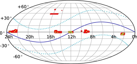
Sky map in equatorial coordinates covered by the Hyper Suprime-Cam Subaru Strategic Program survey between 2014 March and 2016 September. The dots represent the average coordinates of the observed TNOs listed in table 1. The solid and dotted curves show the ecliptic latitudes of 0° and ±30°, respectively. (Color online)
2.2 Data reduction
The data were processed with hscPipe, which is the HSC data reduction/analysis pipeline developed by the HSC collaboration team (Bosch et al. 2018) based on the Large Synoptic Survey Telescope (LSST) pipeline software (Ivezic et al. 2008; Axelrod et al. 2010; Jurić et al. 2015). First, a raw image is reduced by CCD-by-CCD procedures including bias subtraction, linearity correction, flat-fielding, artifacts masking, and background subtraction. Next, the pipeline detects sources and determines the World Coordinate System (WCS) and zero-point magnitude of the corrected data by matching to the Pan-STARRS 1 (PS1) 3π catalog (Tonry et al. 2012; Schlafly et al. 2012; Magnier et al. 2013). Then, the centroids, shapes, and fluxes of detected sources are measured with several different algorithms. We use the sinc aperture flux (Bickerton & Lupton 2013) with 12 pixel (i.e., ∼2|${^{\prime\prime}_{.}}$|0) radius aperture for photometry of TNOs, which is the same configuration as for estimating the zero-point magnitude. Note that the zero points are translated from PS1 into the native HSC system by a color term (Kawanomoto et al. 2017). Lastly, the pipeline generates source catalogs describing the measurement values and flags of detected objects in each CCD. The source catalogs and corrected images are stored in the HSC database, and can be queried by using the Catalog Archive Server (CAS) search3 and quarried by using the Data Archive System (DAS),4 respectively (T. Takata et al. 2017 in preparation).
2.3 Object sample
As of the end of 2016, more than 1700 TNOs have been discovered. The daily ephemeris of each object was retrieved from the Minor Planet & Comet Ephemeris Service website5 managed by the Minor Planet Center. We searched for known TNOs with coordinates located within the area of the HSC-SSP data at the acquisition date, and checked if there was a detected source corresponding to each of those objects in the source catalogs using the sub-hourly ephemeris. The identified source was checked by visual inspection. If the source was judged not to be a TNO (e.g., a star, galaxy, artifact) or had some kind of problem, such as being located at the edge of the image or too close to a very bright object, it was excluded from the color measurement. In addition, we selected objects measured in at least four broad-bands as the targets of this study. Based on the above criteria we finally found 30 TNOs suitable for the present multi-band color investigation in the HSC-SSP data. Table 1 shows these objects and their acquisition dates in each band. Twenty-eight objects were measured in all five broad-bands, and the other two objects (2014 DL143 and 2002 PD155) were measured in four bands.
Measured TNOs and their acquisition dates in each filter.*
| Object | g | r | i | z | Y |
|---|---|---|---|---|---|
| 1994 ES2 | 2015-03-25(1), 2016-04-04(6) | 2016-04-08(1), 2016-06-05(2) | 2015-03-22(1), 2016-04-02(8) | 2015-03-16(1), 2016-06-04(8) | 2015-03-29(1) |
| (60454) 2000 CH105 | 2015-03-25(5) | 2015-03-18(4) | 2015-03-22(1), 2015-03-20(5) | 2015-03-16(4), 2015-05-23(3) | 2015-03-29(5) |
| 2001 DC106 | 2015-03-25(2) | 2015-03-18(3) | 2015-03-20(2) | 2015-03-16(3) | 2015-03-29(3) |
| 2001 DD106 | 2015-03-25(4), 2016-04-04(1) | 2015-03-18(3), 2016-04-08(1) | 2015-03-22(1), 2015-03-20(4) | 2015-03-16(6), 2015-05-23(1) | 2015-03-29(4), 2016-02-12(1), 2016-04-15(1) |
| 2002 CT154 | 2015-03-25(1), 2016-04-04(4) | 2015-03-18(1), 2016-04-08(2) | 2015-03-20(1), 2016-04-02(6) | 2015-03-16(1), 2016-06-04(5) | 2015-03-29(1), 2016-04-15(4) |
| 2002 CY154 | 2015-03-25(2) | 2015-03-18(4) | 2015-03-20(6) | 2015-05-23(4) | 2015-03-29(3), 2015-05-19(2) |
| 2002 FV6 | 2015-03-25(3) | 2015-03-18(2) | 2015-03-20(2), 2015-05-21(2) | 2015-05-23(2) | 2015-03-29(2) |
| 2002 PD155 | 2014-10-01(3), 2016-09-06(1) | 2014-09-22(2), 2016-09-07(1) | 2014-09-22(3) | 2014-10-01(5) | n/a |
| (434194) 2003 FK127 | 2016-04-04(3) | 2016-06-05(1) | 2016-04-02(6) | 2016-06-04(2) | 2016-04-15(4) |
| 2003 FL127 | 2016-04-04(2) | 2016-04-08(4), 2016-06-05(3) | 2016-03-04(2) | 2016-03-12(5), 2016-06-01(4) | 2016-02-03(3) |
| (120178) 2003 OP32 | 2016-07-07(2) | 2016-06-11(3), 2016-09-02(3) | 2016-07-05(4), 2016-08-30(1), 2016-08-28(1) | 2016-06-04(3), 2016-06-01(1), 2016-07-12(3) | 2016-08-09(8), 2016-07-31(4) |
| (183963) 2004 DJ64 | 2016-04-04(6) | 2016-06-05(1) | 2016-04-02(8) | 2016-06-04(6) | 2016-04-15(7) |
| 2004 DM71 | 2016-04-04(5) | 2016-06-05(3) | 2016-04-02(7) | 2016-06-04(3) | 2016-04-15(2) |
| 2005 GX186 | 2016-04-04(7) | 2016-06-05(5) | 2016-04-02(8) | 2016-06-04(5) | 2016-04-15(3) |
| (145452) 2005 RN43 | 2014-09-18(2), 2015-07-14(5) | 2014-09-22(2), 2015-07-15(5) | 2014-11-23(2), 2015-07-21(5) | 2014-09-28(1), 2015-07-22(3), 2015-08-20(1) | 2014-09-18(2), 2015-07-23(5) |
| 2008 SO266 | 2015-10-14(3) | 2015-10-10(4) | 2015-11-10(5) | 2015-11-06(1), 2016-01-12(2) | 2015-10-20(7), 2015-10-06(1) |
| 2012 VR113 | 2014-10-01(1), 2014-11-18(3), 2015-10-14(2) | 2014-11-18(2), 2015-10-10(2) | 2014-09-22(1), 2014-11-28(2), 2014-11-23(1) | 2014-10-01(2), 2015-11-06(3) | 2014-09-18(1), 2014-11-28(5), 2015-10-20(3) |
| 2013 QO95 | 2014-10-01(3), 2014-11-18(4), 2015-10-14(4) | 2014-11-18(4), 2015-10-10(4) | 2014-09-22(6), 2015-01-21(1) | 2014-10-01(6), 2014-11-25(1), 2014-11-21(2) | 2014-09-18(4), 2014-11-21(2), 2016-01-09(5) |
| 2013 QP95 | 2014-10-01(6), 2014-11-18(6), 2015-10-14(1) | 2014-11-28(4), 2014-11-18(9), 2015-10-10(2) | 2014-09-22(8), 2014-11-23(11) | 2014-10-01(6), 2014-11-25(4), 2014-11-21(7), 2015-11-06(4) | 2014-09-18(7), 2014-11-21(14), 2016-01-09(2) |
| 2013 RD98 | 2014-10-01(4), 2014-11-25(1), 2014-11-18(4), 2015-10-14(3) | 2014-11-18(5), 2015-10-10(2) | 2014-09-22(5), 2014-11-23(6) | 2014-10-01(2), 2014-11-25(2), 2014-11-21(5), 2016-01-12(3) | 2014-09-18(1), 2015-10-06(2) |
| 2014 DL143 | 2016-04-04(6) | 2016-06-05(5) | 2016-04-02(2) | n/a | 2016-04-15(2), 2016-06-28(2) |
| 2014 GS53 | 2015-05-17(7), 2016-04-04(6) | 2015-07-13(2), 2016-03-09(3) | 2015-05-21(3), 2016-04-09(8) | 2015-07-12(7), 2016-03-12(5) | 2014-03-25(2), 2015-05-26(5), 2016-03-15(7), 2016-03-14(2) |
| 2014 GX53 | 2015-03-25(1), 2015-05-17(2) | 2015-03-18(1), 2015-05-15(2) | 2014-03-28(7), 2015-03-22(4), 2015-03-20(2) | 2015-03-29(1), 2015-05-23(5), 2015-05-13(1) | 2014-03-25(8), 2015-03-29(1), 2015-05-19(7) |
| 2014 NB66 | 2015-10-14(1), 2016-07-07(5) | 2016-07-03(3) | 2016-07-05(2), 2016-08-30(2) | 2016-07-29(3) | 2016-07-31(6) |
| (483002) 2014 QS441 | 2014-11-25(3) | 2014-11-28(2), 2014-11-18(1) | 2014-11-23(2), 2015-01-21(5), 2015-08-11(4) | 2014-11-25(5), 2015-01-16(4), 2015-08-20(11), 2016-08-01(4) | 2014-11-28(3), 2015-08-09(11) |
| 2014 TU85 | 2014-11-18(3) | 2014-11-18(3) | 2014-09-22(5), 2014-11-23(5), 2015-01-21(2) | 2014-10-01(1), 2014-11-25(2), 2014-11-21(1), 2015-01-16(1) | 2014-09-18(1) |
| 2014 UF224 | 2014-10-01(4), 2014-11-18(10), 2015-10-14(5) | 2014-11-28(5), 2014-11-18(10), 2015-10-10(5) | 2014-09-22(5), 2014-11-23(11), 2015-11-14(1), 2016-02-09(2) | 2014-10-01(3), 2014-11-25(8), 2014-11-21(7), 2015-11-06(5), 2016-01-12(9) | 2014-11-21(6) |
| 2014 WZ509 | 2015-03-25(1) | 2015-03-18(1) | 2015-01-21(8) | 2015-01-16(6), 2015-11-06(4) | 2015-01-27(6), 2015-10-20(1), 2016-01-09(1) |
| 2015 FM345 | 2015-05-17(5), 2016-04-04(3) | 2015-07-13(1), 2016-04-08(1) | 2015-05-21(1), 2016-04-09(8) | 2015-07-12(8), 2016-03-12(3) | 2015-05-26(4), 2016-03-15(4) |
| 2015 QT11 | 2015-10-14(3) | 2014-11-18(1), 2015-10-10(4) | 2014-11-23(2), 2016-02-09(1) | 2014-11-25(1) | 2015-10-06(2) |
*The number of shots taken on each date is also displayed in parentheses.
The semi-major axis (a), eccentricity (e), and inclination (I) of our target objects are listed in table 2. According to the Deep Ecliptic Survey (DES) online classification,6 the sample includes four TNOs located at mean motion resonances (MMR) with Neptune, three in the 3:2 MMR (2003 FL127, 2008 SO266, and 2013 RD98) and one in the 2:1 MMR (2012 VR113). Next, we divided the non-resonant TNOs in our sample into two dynamical classes: classical and scattered TNOs. Based on the classification scheme presented by Lykawka and Mukai (2007)— see also Gladman, Marsden, and Vanlaerhoven (2008)— the former objects have orbits with semi-major axes of 37 au < a < 47.5 au and perihelion distance q > 37 au, while the latter ones have orbits with 30 au < q < 37 au. Using the above definition, we classified 19 objects as classical TNOs and 7 objects as scattered TNOs. There was no object corresponding to the detached population in our sample.
Target TNOs.*
| Object | a | e | I | Class | Hg | Hr | Hi | Hz | HY |
|---|---|---|---|---|---|---|---|---|---|
| (au) | (°) | (mag) | (mag) | (mag) | (mag) | (mag) | |||
| 1994 ES2 | 46.158 | 0.12 | 1.1 | Cold classical | 8.66 ± 0.39 | 7.38 ± 0.25 | 6.74 ± 0.24 | 6.10 ± 0.51 | 7.64 ± 1.74 |
| 2000 CH105 | 44.636 | 0.09 | 1.2 | Cold classical | 7.52 ± 0.21 | 6.23 ± 0.14 | 5.70 ± 0.11 | 5.47 ± 0.11 | 5.32 ± 0.27 |
| 2001 DC106 | 42.488 | 0.06 | 1.9 | Cold classical | 7.52 ± 0.11 | 6.22 ± 0.12 | 5.43 ± 0.07 | 5.07 ± 0.11 | 5.16 ± 0.23 |
| 2001 DD106 | 44.338 | 0.10 | 1.8 | Cold classical | 8.60 ± 0.34 | 7.39 ± 0.10 | 6.63 ± 0.22 | 6.34 ± 0.28 | 6.05 ± 0.57 |
| 2002 CT154 | 47.159 | 0.12 | 3.5 | Cold classical | 7.79 ± 0.20 | 6.83 ± 0.17 | 5.87 ± 0.19 | 5.84 ± 0.15 | 5.48 ± 0.38 |
| 2002 CY154 | 44.564 | 0.07 | 1.0 | Cold classical | 7.93 ± 0.27 | 6.57 ± 0.12 | 5.86 ± 0.12 | 5.69 ± 0.34 | 4.86 ± 0.45 |
| 2002 FV6 | 47.267 | 0.15 | 3.1 | Cold classical | 8.01 ± 0.31 | 6.13 ± 0.12 | 5.78 ± 0.17 | 5.52 ± 0.36 | 4.90 ± 0.39 |
| 2002 PD155 | 43.051 | 0.00 | 5.8 | Cold classical | 8.28 ± 0.28 | 7.14 ± 0.74 | 6.53 ± 0.13 | 6.61 ± 0.26 | n/a |
| 2003 FK127 | 42.878 | 0.06 | 2.3 | Cold classical | 8.02 ± 0.16 | 6.44 ± 0.10 | 6.14 ± 0.12 | 5.47 ± 0.47 | 5.83 ± 0.40 |
| 2003 FL127 | 39.461 | 0.23 | 3.5 | Resonant | 7.79 ± 0.17 | 6.33 ± 0.12 | 5.50 ± 0.22 | 5.35 ± 0.20 | 5.01 ± 0.16 |
| 2003 OP32 | 43.086 | 0.11 | 27.2 | Hot classical | 4.18 ± 0.09 | 3.62 ± 0.14 | 3.20 ± 0.11 | 3.11 ± 0.09 | 3.03 ± 0.08 |
| 2004 DJ64 | 44.698 | 0.11 | 2.4 | Cold classical | 7.68 ± 0.17 | 6.99 ± 0.12 | 6.20 ± 0.15 | 6.32 ± 0.59 | 5.55 ± 0.27 |
| 2004 DM71 | 43.383 | 0.03 | 2.3 | Cold classical | 8.33 ± 0.19 | 7.12 ± 0.14 | 6.59 ± 0.11 | 6.46 ± 0.39 | 7.18 ± 1.14 |
| 2005 GX186 | 44.273 | 0.03 | 3.8 | Cold classical | 7.68 ± 0.21 | 6.29 ± 0.12 | 6.15 ± 0.15 | 5.60 ± 0.24 | 5.46 ± 0.60 |
| 2005 RN43 | 41.379 | 0.02 | 19.3 | Hot classical | 4.33 ± 0.06 | 3.32 ± 0.04 | 2.75 ± 0.04 | 2.45 ± 0.07 | 2.34 ± 0.06 |
| 2008 SO266 | 39.236 | 0.24 | 18.8 | Resonant | 7.25 ± 0.07 | 6.23 ± 0.09 | 5.42 ± 0.10 | 5.21 ± 0.12 | 4.95 ± 0.13 |
| 2012 VR113 | 47.466 | 0.17 | 19.3 | Resonant | 7.11 ± 0.12 | 6.21 ± 0.05 | 5.72 ± 0.10 | 5.52 ± 0.20 | 5.32 ± 0.30 |
| 2013 QO95 | 39.822 | 0.03 | 20.6 | Hot classical | 7.86 ± 0.31 | 6.42 ± 0.10 | 5.97 ± 0.34 | 5.54 ± 0.15 | 5.19 ± 0.47 |
| 2013 QP95 | 40.488 | 0.17 | 25.5 | Scattered | 7.68 ± 0.28 | 7.00 ± 0.10 | 6.47 ± 0.09 | 6.13 ± 0.15 | 6.05 ± 0.54 |
| 2013 RD98 | 39.315 | 0.23 | 19.6 | Resonant | 7.82 ± 0.17 | 7.03 ± 0.13 | 6.59 ± 0.27 | 6.24 ± 0.36 | 5.80 ± 0.33 |
| 2014 DL143 | 47.332 | 0.22 | 9.3 | Scattered | 6.71 ± 0.08 | 5.97 ± 0.09 | 5.22 ± 0.10 | n/a | 5.01 ± 0.31 |
| 2014 GS53 | 33.622 | 0.10 | 15.2 | Scattered | 7.41 ± 0.09 | 6.14 ± 0.16 | 5.37 ± 0.09 | 5.01 ± 0.12 | 4.83 ± 0.13 |
| 2014 GX53 | 40.988 | 0.14 | 14.5 | Scattered | 6.03 ± 0.11 | 4.98 ± 0.03 | 4.59 ± 0.10 | 4.24 ± 0.11 | 4.03 ± 0.10 |
| 2014 NB66 | 45.476 | 0.08 | 4.9 | Cold classical | 5.96 ± 0.19 | 5.49 ± 0.12 | 4.70 ± 0.12 | 4.12 ± 0.10 | 4.40 ± 0.28 |
| 2014 QS441 | 46.774 | 0.07 | 38.0 | Hot classical | 5.64 ± 0.14 | 5.14 ± 0.09 | 4.85 ± 0.06 | 4.74 ± 0.09 | 4.82 ± 0.33 |
| 2014 TU85 | 48.647 | 0.31 | 16.4 | Scattered | 8.92 ± 0.38 | 7.93 ± 0.26 | 7.64 ± 0.25 | 7.25 ± 0.38 | 6.88 ± 0.42 |
| 2014 UF224 | 45.273 | 0.13 | 27.2 | Hot classical | 7.52 ± 0.25 | 6.94 ± 0.17 | 6.43 ± 0.26 | 6.07 ± 0.34 | 5.79 ± 0.29 |
| 2014 WZ509 | 40.431 | 0.09 | 15.9 | Scattered | 5.87 ± 0.09 | 5.17 ± 0.09 | 4.67 ± 0.05 | 4.40 ± 0.20 | 4.39 ± 0.15 |
| 2015 FM345 | 42.862 | 0.04 | 17.1 | Hot classical | 7.23 ± 0.30 | 6.27 ± 0.09 | 5.29 ± 0.14 | 5.20 ± 0.23 | 5.02 ± 0.41 |
| 2015 QT11 | 38.676 | 0.07 | 26.6 | Scattered | 9.03 ± 0.17 | 8.15 ± 0.16 | 8.13 ± 0.64 | 7.44 ± 0.40 | 6.79 ± 0.26 |
*Semi-major axis (a), eccentricity (e), inclination (I), dynamical classification, and measured absolute magnitudes (H) in the g, r, i, z, and Y bands.
Furthermore, the classical TNOs contain a swarm of objects with inclination smaller than 6°, generally called “cold classical TNOs.” We divided the classical TNOs into two sub-populations with a boundary of inclination I = 6°, 13 cold (I < 6°) and 6 hot (I > 6°) objects. The a vs. e and a vs. I plots of our samples with the above classification are shown in figure 2.
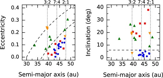
Semi-major axis vs. eccentricity (left) and semi-major axis vs. inclination (right) plots of our TNO sample. Our 30 target TNOs are shown according to distinct dynamical classes: cold classical (circles), hot classical (squares), scattered (triangles), and resonant objects (inverse triangles), respectively. The vertical dotted lines show the locations of the 3:2, 7:4, and 2:1 mean motion resonances with Neptune. The dashed curves in the left panel show the perihelion distances of 30 au and 37 au. The dashed curve in the right panel shows an inclination of 6°. (Color online)
2.4 Color measurements
Rabinowitz, Schaefer, and Tourtellotte (2007) examined the plot of B- and I-band phase coefficients obtained from 18 TNOs and 7 Centaurs (see figure 3 of their paper). Although there are several outliers among the TNOs, most of the objects have comparable values between the two bands. Using a sample of 52 icy bodies including TNOs, Centaurs, and planetary satellites, Schaefer, Rabinowitz, and Tourtellotte (2009) also showed that in general the phase curve slope in the B band differs from that in the I band by less than ∼0.02 mag deg−1. These data imply that the phase coefficient of TNOs can almost be regarded as wavelength independent. We assume a constant value of β = 0.11 mag deg−1 (Alvarez-Candal et al. 2016) for all the bands.
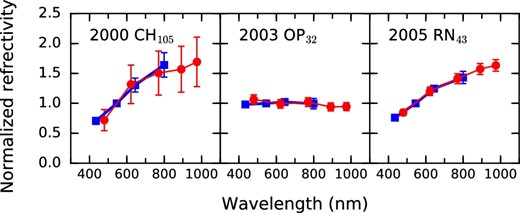
Normalized reflectance spectra of the objects whose colors were previously measured and compiled in the “Minor Bodies in the Outer Solar System” (MBOSS) database (Hainaut & Delsanti 2002; Hainaut et al. 2012). The circles and squares show the color data obtained by the present work from the HSC-SSP survey (g, r, i, z, and Y bands) and those compiled in MBOSS (B, V, R, and I bands), respectively. (Color online)
We estimate the color from the differences between Hx values, e.g., Hg − Hr for the g − r color. The deviation of the Hx value from the mean magnitude level of the lightcurve (ΔHx) could cause an additional uncertainty in the color measurement. According to the analysis by Duffard et al. (2009), the mean rotation period and lightcurve amplitude of TNOs are 6.95 hr and 0.25 mag, respectively. Using a Monte Carlo method, we generated synthetic lightcurves assuming a sinusoidal brightness fluctuation with 6.95 hr period, 0.25 mag amplitude, and random initial phase angles, and computed the standard deviation (|$\sigma _{\Delta H_x}$|) of ΔHx values at the actual acquisition epochs of each object/band. Then, the total Hx uncertainty is obtained by |$\sqrt{ \sigma _{H_x}^2 + \sigma _{\Delta H_x}^2 }$|. The Hx magnitudes and uncertainties obtained for all the sample objects are shown in table 2. Note that the magnitudes and colors are expressed in the Vega magnitude system hereafter.
Three of our sample objects have been observed with multi-band imaging by previous studies: (60454) 2000 CH105 (Peixinho et al. 2004; Benecchi et al. 2011), (120178) 2003 OP32 (Perna et al. 2010, 2013; Rabinowitz et al. 2008), and (145452) 2005 RN43 (DeMeo et al. 2009; Perna et al. 2013), and are also listed in the “Minor Bodies in the Outer Solar System” (MBOSS) database (Hainaut & Delsanti 2002; Hainaut et al. 2012). The reflectance spectra of these objects obtained from the MBOSS color data and our measurements are shown in figure 3. The solar colors were given by Holmberg, Flynn, and Portinari (2006) and were corrected into the HSC band system with color term conversion (see table 3).
Colors of the Sun in the Vega magnitude system.
| Color | SDSS* | HSC | ||
|---|---|---|---|---|
| g − r | 0.70 | 0.63 | ||
| r − i | 0.35 | 0.39 | ||
| i − z | 0.21 | 0.18 | ||
| z − Y | — | 0.07 |
| Color | SDSS* | HSC | ||
|---|---|---|---|---|
| g − r | 0.70 | 0.63 | ||
| r − i | 0.35 | 0.39 | ||
| i − z | 0.21 | 0.18 | ||
| z − Y | — | 0.07 |
*Take from Holmberg, Flynn, and Portinari (2006).
In the range of wavelengths where the two datasets overlap, namely from 0.5 μm to 0.8 μm, we confirmed that the two spectra agree well with each other for the three objects illustrated in figure 3, indicating that our measurements have sufficient accuracy. Note that our color data in the wavelength range from 0.4 μm to 1.0 μm are useful to complement the spectral coverage between the I (∼0.8 μm) and J (∼1.25 μm) bands. To our knowledge, except for the three aforementioned objects, the visible colors of our sample objects were measured for the first time by our present study.
3 Results
First, we examine the colors derived from the absolute magnitudes in two adjacent bands. Figure 4 shows the histogram plots of the sample objects in the g − r, r − i, i − z, and z − Y colors, separately displayed for each dynamical population. The dashed lines represent the solar color. This figure reveals the following properties: (1) The hot classical and scattered populations have similar color distributions, with a peak close to the solar color in all the band pairs. (2) The cold classical population exhibits a redder distribution compared to the hot classical and scattered populations in the g − r and r − i colors, while their i − z and z − Y colors are distributed around the solar color. (3) The resonant objects concentrate close to the solar color in the i − z and z − Y bands, but their colors apparently range from neutral to red in g − r and r − i colors. These findings are consistent with the results of, e.g., Gulbis, Elliot, and Kane (2006), Peixinho, Lacerda, and Jewitt (2008), and Benecchi et al. (2011).
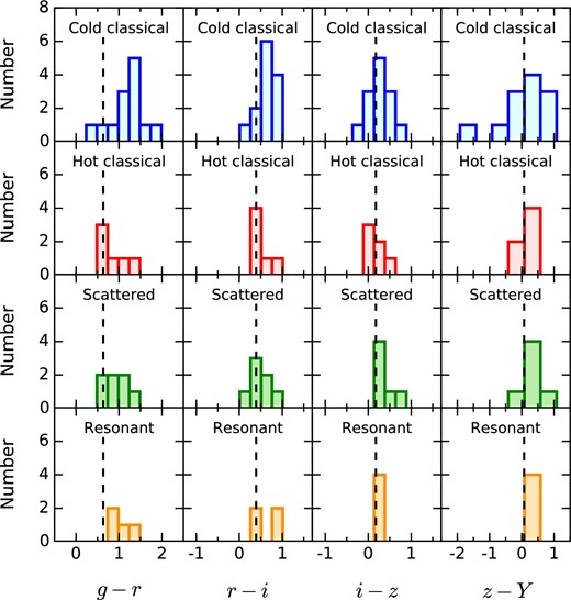
Color distributions of our target TNOs according to their dynamical classes. From top to bottom, the rows show the cold classical, hot classical, scattered, and resonant populations. The dashed lines show the solar color.
Figure 5 illustrates the color–color diagrams of the sample objects, separately displayed for each dynamical population. The star symbol shows the solar colors. The dashed line indicates a color track given from linear reflectance spectra called the “reddening line” (Hainaut & Delsanti 2002), which is useful for understanding the shape of spectra. Objects above/below the line have a slope increase/decrease toward longer wavelength, respectively, over the wavelength range of the two colors. In the i − z vs. z − Y plot, most of the objects are located on the upper right side from the solar color along the reddening line, suggesting that the typical reflectance spectra of TNOs are flat or linearly increasing with wavelength between the i and Y bands regardless of the dynamical population. Such a distribution is also seen for the hot classical and scattered populations in the g − r vs. r − i and r − i vs. i − z plots. On the other hand, the cold classical objects show a significant deviation to the right side of the reddening line in the g − r vs. r − i and potentially r − i vs. i − z plots, indicating a steeper slope in the short wavelength range. These properties can also be confirmed in the average reflectance spectra shown in figure 6. The spectra of the hot classical and scattered populations are approximated by linear slopes over all five bands, but the reflectance spectra of the cold classical population show a steep increase at the short wavelength edge.
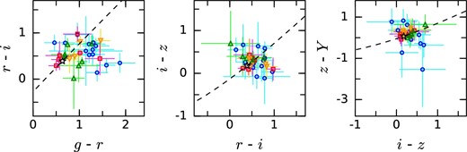
Color–color diagrams of our target TNOs according to distinct dynamical classes: cold classical (circles), hot classical (squares), scattered (triangles), and resonant objects (inverse triangles). The star symbol shows the solar colors. The dashed curves show the reddening lines (see text).
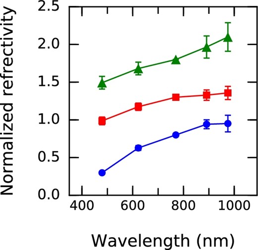
Average reflectance spectra of the cold classical (circles), hot classical (squares), and scattered (triangles) populations, which have been normalized at the i band and vertically shifted for clarity. (Color online)
By comparing the color plots of the dynamical populations in figures 4, 5, and 6, it appears that the hot classical and scattered populations have similar color distributions, while the cold classical population exhibits a different spectral property, especially in the short wavelength range. In the following, we investigate the similarity of the color distributions among the populations using two statistical tests based on Press et al. (2002).
Results of Student’s t-test and Kolmogorov–Smirnov (KS) test.
| Populations | Color | P t* | P KS † |
|---|---|---|---|
| Cold classical vs. hot classical | g − r | 0.04 | 0.06 |
| r − i | 0.57 | 0.28 | |
| Cold classical vs. scattered | g − r | 0.01 | 0.03 |
| r − i | 0.12 | 0.34 | |
| Hot classical vs. scattered | g − r | 0.34 | 0.28 |
| r − i | 0.48 | 0.95 |
*Probabilities for the null hypothesis in the t test.
†Probabilities for the null hypothesis in the KS test.
In addition to the color properties, considering the Tisserand parameter with respect to Neptune, TN,7 the low-I and high-I populations have TN > 3.0 and TN < 3.0, respectively, except for one scattered object, 2014 DL143 (see figure 7). Thus, the division of our sample into the low- and high-I populations is based on both physical (colors) and dynamical (TN) grounds. 2014 DL143 has a perihelion distance of 36.92 au, close to the boundary between the classical and scattered TNOs, and an inclination of 9.°3, which is by far the smallest in the high-I population. This object could have intermediate dynamical characteristics between the cold/hot classical and scattered TNOs, while its g − r color, 0.75 ± 0.12, is closer to the color distribution peaks of the hot classical and scattered TNOs rather than that of the cold classical TNOs. In this paper, 2014 DL143 was classified into the high-I population.
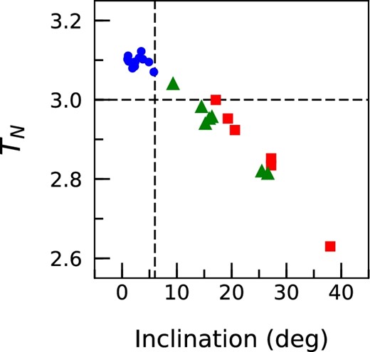
Inclination (I) vs. Tisserand parameter with respect to Neptune (TN) plot of our target TNOs according to their dynamical classes: cold classical (circles), hot classical (squares), and scattered (triangles). The vertical and horizontal dashed lines represent I = 6° and TN = 3.0, respectively. (Color online)
Figure 8 shows the color distributions of the low-I and high-I populations. It is clear that the two populations differ in the g − r and r − i color distributions. However, both populations are indistinguishable from each other in the i − z and z − Y color distributions. The high-I objects concentrate around the solar color in all the colors, with slight reddening with wavelength. In contrast, most of the low-I objects are notably redder than the solar color in the g − r distribution, but the peak approaches neutral in the long wavelength range (see also figure 6). This spectral distinction between these two populations may be caused by differences in their origin and/or evolution. In the next section, we analyze the characteristics of the low-/high-I populations, as well as their correlations with other parameters.
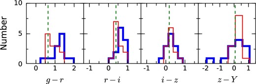
Color distributions of the low-I (thick line) and high-I (thin line) populations, defined by I < 6° and I > 6°, respectively. The dashed lines show the solar color.
4 Discussion
4.1 Correlations
Examination of the correlations between the TNO colors and the other parameters such as orbital elements could give us important clues on the origin and dynamical/chemical evolutions of TNOs. In particular, comparison of such correlations may be useful to better understand the cause of similarities/differences in the color properties. We assessed correlations of colors with the semi-major axis, perihelion distance, eccentricity, inclination, and absolute magnitude with the i band. The obtained colors vs. these parameters are displayed in figure 9.
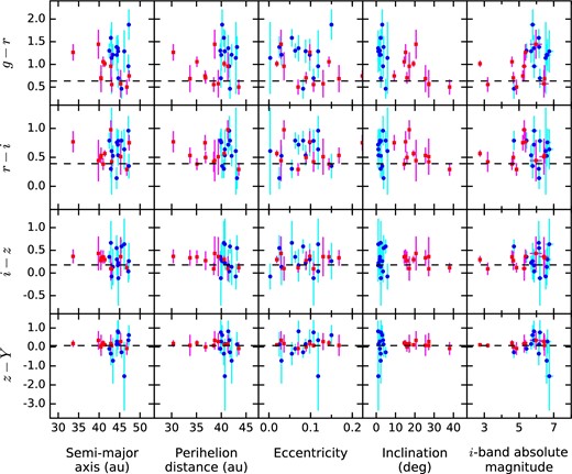
Colors vs. orbital elements and absolute magnitude of the low-I (circles) and high-I (squares) populations. The dashed lines show the solar color.
We referred to the JPL Small-Body Database Browser8 for information regarding the precision of orbit determination of the individual objects. As of 2017 March, we found that 28 of them have sufficiently accurate orbits, but 2014 TU85 and 2015 QT11 have large orbital uncertainties in both semi-major axis and eccentricity (Δa ∼ 22.2 au and Δe ∼ 0.58 for 2014 TU85, Δa ∼ 0.85 au and Δe ∼ 0.36 for 2015 QT11, where Δa and Δe are the 1 σ uncertainties in the semi-major axis and eccentricity, respectively). Therefore, these two objects were excluded from the following analysis of correlations.
Table 5 shows the results of the correlation tests. We found significant correlations between colors and inclinations for all the samples. Notably, the g − r color exhibits strong anti-correlation with inclination (Pt ∼ 0.0003), in agreement with previous studies (e.g., Trujillo & Brown 2002; Doressoundiram et al. 2008; Peixinho et al. 2008; Hainaut et al. 2012). In contrast, the other parameters investigated are not significantly correlated with the colors.
Results of the correlation tests.*
| All | Low-I | High-I | ||||||
|---|---|---|---|---|---|---|---|---|
| r s | P t | r s | P t | r s | P t | |||
| g − r vs. a | −0.15 | 0.73 | −0.31 | 0.14 | −0.39 | 0.07 | ||
| r − i vs. a | −0.07 | 0.33 | 0.03 | 0.09 | −0.39 | 0.53 | ||
| g − r vs. q | 0.10 | 0.49 | −0.27 | 0.84 | −0.31 | 0.12 | ||
| r − i vs. q | 0.02 | 0.10 | −0.41 | 0.08 | −0.31 | 0.13 | ||
| g − r vs. e | −0.22 | 0.08 | 0.07 | 0.22 | −0.08 | 0.27 | ||
| r − i vs. e | 0.08 | 0.37 | 0.46 | 0.06 | −0.08 | 0.03 | ||
| g − r vs. I | −0.60 | ≪0.01 | −0.19 | 0.57 | −0.54 | 0.02 | ||
| r − i vs. I | −0.37 | 0.02 | 0.05 | 0.18 | −0.54 | 0.06 | ||
| g − r vs. Hi | 0.19 | 0.10 | −0.21 | 0.63 | 0.04 | 0.15 | ||
| r − i vs. Hi | −0.21 | 0.09 | −0.35 | 0.12 | 0.04 | 0.72 | ||
*Significance of correlation between the colors and other parameters including semi-major axis (a), perihelion distance (q), eccentricity (e), inclination (I), and i-band absolute magnitude (Hi), for all the objects and for the low-/high-I populations separately. rs and Pt represent the Spearman rank-order correlation coefficient and the probability for the null hypothesis (no correlation), respectively. Small Pt with positive/negative rs implies a high degree of positive/negative correlation.
We also examined correlations for each of the low-/high-I populations in the same manner. The high-I population exhibits a moderate correlation between the g − r color and inclination, while the low-I population does not show such a trend. This may indicate that the correlation between color and inclination is not continuous across all data values, but is limited to the objects in the high-I population. If so, the low-/high-I populations could represent distinct populations with different origins or dynamical evolutions.
4.2 g − i color
As discussed in section 3, figure 8 illustrates that the low-/high-I populations seem to have different g − r and r − i color distributions. As suggested in previous works (e.g., Wong & Brown 2016, 2017), we take the g − i color as a useful index to characterize the two populations.
Figure 10 shows the g − i color distributions for the two populations. There is a clear distinction that the high-I population exhibits a peak around the solar color (0.75 ≲ g − i ≲ 1.25) while the low-I population has no corresponding objects near the solar color. The g − i color of the high-I distribution extends up to g − i ∼ 2.25, which corresponds to the higher end of the g − i distribution for the low-I population. Wong and Brown (2017) reported that the hot TNO population with I ≥ 5° has a bimodal distribution in the g − i color, “red” (R; g − i ≤ 1.53) and “very red” (VR; g − i ≥ 1.81) sub-populations. The high-I population of our data covers a similar range in g − i color to Wong and Brown (2017), but the small number of statistics prevent us from confirming bimodality. We note that the peak location of their VR population, g − i ∼ 1.9, agrees with that of the low-I distribution in our data.
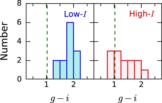
g − i color distributions of the low-I (left) and high-I (right) populations. The dashed lines show the solar color.
Furthermore, we also found a notable relationship between the g − i color and orbital elements. Figure 11 illustrates g − i color vs. eccentricity and g − i color vs. inclination for the low-/high-I populations. The g − i color vs. eccentricity distribution seems to be divided into two swarms. The first swarm consists of low eccentricity (e ≲ 0.1) and red objects (g − i ≳ 1.5), and the second one consists of objects with relatively high eccentricity (e ≳ 0.1) and close to the neutral color. The former is dominated by the low-I population, while the latter is dominated by the high-I population.
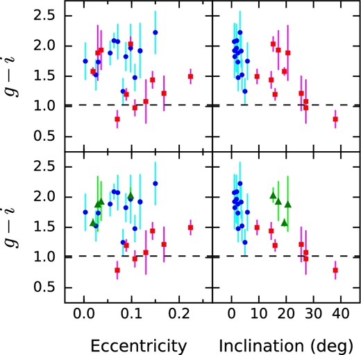
Top: g − i color vs. eccentricity/inclination of the low-I (circles) and high-I (squares) populations. Bottom: As the top panels, but the red high-I objects are marked with triangles. The dashed lines show the solar color.
The g − i vs. eccentricity plot also shows that four high-I objects with low eccentricity (2005 RN43, 2013 QO95, 2014 GS53, and 2015 FM345) are located in the low-e/red swarm. Intriguingly, these objects are concentrated at a < 43 au and I < 21°. Taken together with their redder g − i colors, these results suggest that the high-I population would consist of two distinct components, in agreement with the findings of Wong and Brown (2017). In particular, these four TNOs could be members of the VR TNOs, while the other high-I TNOs would not belong to the VR group (furthermore, most of them are even less red than the mean g − i color of the R TNOs). If we focus the analysis solely on the latter group, after excluding these four objects, the g − i distribution of the high-I population exhibits a positive correlation with eccentricity and negative correlation with inclination with high significance levels (Pt ∼ 0.004 and 0.0005, respectively). This may reflect the relationship among orbits, colors, and dynamical evolution of the neutral-color high-I population, as well as possibly different origins/evolutions between the red and neutral high-I objects. These two sub-populations of high-I objects probably form the color bimodality presented in Wong and Brown (2017), although the color distribution of the neutral high-I objects does not correspond to that of the R TNOs. While further data are required for detailed investigation, the presence of the red high-I objects has potential for being an essential clue for understanding the cause of difference in reflectance spectra between low-I and high-I populations.
4.3 Interpretation
Our analysis shows that: (1) the hot classical and scattered populations have similar reflectance spectra with a constant (flat or reddish) slope in the wavelength range at least from 0.4 μm to 1.0 μm; (2) the cold classical population exhibits distinctive spectra with reflectance increasing below the i band (∼0.8 μm) with a steeper slope at the short wavelength end (≲0.6 μm); (3) the high-I population shows an anti-correlation between g − r/r − i colors and inclination; (4) for the high-I TNOs with less-red color, there is a strong anti-correlation between g − i color and inclination. The depth, shape, and wavelength range of this reflectance decay is potentially useful for elucidating the reddening mechanism as well as the factor of the color diversity of TNOs, which can provide a unique constraint on the origins and evolutions of these populations.
The difference in the color distributions among the dynamical classes and the color–inclination correlation have been noted in previous studies (e.g., Doressoundiram et al. 2008; Hainaut et al. 2012; Peixinho et al. 2015; Wong & Brown 2017). Two main hypotheses have been proposed to explain these features, as we describe below.
4.3.1 Collisional resurfacing
The diversity of colors would reflect different collisional evolutions experienced by the TNOs. While giant impacts may darken the surfaces of large TNOs (Sekine et al. 2017), it is often thought that impacts excavate surfaces reddened by space weathering (Doressoundiram et al. 2008). In particular, objects with dynamically excited orbits, i.e., with high eccentricity and/or inclination, can suffer more energetic collisions. Such impacts can excavate the surface layers covered by irradiated reddish materials, thus exposing the subsurface fresh (neutral color) materials. Hainaut, Boehnhardt, and Protopapa (2012) reported an anti-correlation between color and the orbital excitation parameter |$\varepsilon = \sqrt{e^2 + \sin ^2 I}$| among the hot classical objects. However, this parameter seems mostly dominated by the inclinations, since most of the classical objects have moderately low eccentricities (e ≲ 0.2). The color–ε correlation possibly reflects nothing but the color–inclination correlation. Thébault and Doressoundiram (2003) argued that the colors of TNOs under collisional resurfacing should have a much stronger correlation with eccentricity than with inclination. The present work shows no correlation between color and eccentricity in the low-I population, which has a narrow range of inclinations. Therefore, our results do not seem to support the collisional resurfacing scenario for TNO color diversity.
4.3.2 Formation sites
The diversity of colors would reflect the distinct formation environments. That is, the birthplaces of TNOs distributed across the protoplanetary disk in the early solar system. Based on recent planetary migration models, the high-I population would consist of objects transported from the inner regions of the disk due to migration of the giant planets, while the low-I population would have formed near its present location (e.g., Levison et al. 2008; Wolff et al. 2012; Fraser et al. 2014). This suggests that the low-I TNOs remained on more distant orbits than the high-I TNOs since their formation, thus allowing them to retain some volatile ices on their surfaces, such as CH3OH, NH3, CO2, H2S, and C2H6 (e.g., Brown et al. 2011; Wong & Brown 2016). These ices are considered to be able to create red material such as organics via irradiation by energetic particles and UV (e.g., Moroz et al. 2003; Brunetto et al. 2006).
In contrast, the surfaces of objects formed in the inner regions with the temperature beyond the sublimation points of such ices maintain the original (neutral) color. Assuming this hypothesis, the similarity of color distribution between the hot classical and scattered population seems to indicate a common origin. Furthermore, the close anti-correlation between g − i color and inclination of the high-I population with relatively high eccentricities, and the existence of the reddish high-I objects with low eccentricities, could provide useful information about their dynamical evolution processes.
5 Summary
We measured the visible five-band colors of 30 known TNOs using the HSC-SSP survey data. The object sample contains 13 cold classical, 6 hot classical, 7 scattered, and 4 resonant TNOs.
The color distributions of the hot classical and scattered populations have peaks close to the solar color in all the colors examined in this work, while the cold classical population shows deviations toward redder colors in the g − r and r − i distributions. Statistical tests suggest that the hot classical and scattered populations share the same color property that the reflectance spectra are approximately linear. On the other hand, the cold classical population deviates from the “reddening line” in the g − r vs. r − i diagram, indicating that its reflectance spectra have a steep increase at the short wavelength edge. This leads us to divide the samples (excluding resonant objects) into two groups, the low-I population consisting of the cold classical objects and the high-I population consisting of the hot classical and scattered objects.
The whole sample exhibits a significant anti-correlation between g − r/r − i colors and inclination. This correlation has also been detected in the high-I population, but not in the low-I population, suggesting that this relationship is probably not continuous over the entire inclination range.
The g − i color is a useful index to characterize the low-/high-I populations. In agreement with the findings of Wong and Brown (2017), our high-I population data support the bimodal distribution in g − i. We also found that the sample can be separated into two swarms in the g − i vs. eccentricity plot: red/low-e and neutral/high-e groups. Although most of the high-I objects are contained in the neutral/high-e group, four of them are located in the red/low-e region. Excluding these objects, the g − i color of the high-I population exhibits a highly significant positive correlation with eccentricity and negative correlation with inclination. Our results showed that these color properties of TNOs can provide important and useful clues for a better understanding of the formation and evolution of small bodies in the outer solar system.
Acknowledgements
This study is based on data collected at Subaru Telescope and retrieved from the HSC data archive system, which are operated by Subaru Telescope and Astronomy Data Center, National Astronomical Observatory of Japan.
The Hyper Suprime-Cam (HSC) collaboration includes the astronomical communities of Japan and Taiwan, and Princeton University. The HSC instrumentation and software were developed by the National Astronomical Observatory of Japan (NAOJ), the Kavli Institute for the Physics and Mathematics of the Universe (Kavli IPMU), the University of Tokyo, the High Energy Accelerator Research Organization (KEK), the Academia Sinica Institute for Astronomy and Astrophysics in Taiwan (ASIAA), and Princeton University. Funding was contributed by the FIRST program from the Japanese Cabinet Office, the Ministry of Education, Culture, Sports, Science and Technology (MEXT), the Japan Society for the Promotion of Science (JSPS), the Japan Science and Technology Agency (JST), the Toray Science Foundation, NAOJ, Kavli IPMU, KEK, ASIAA, and Princeton University.
This paper makes use of software developed for the Large Synoptic Survey Telescope. We thank the LSST Project for making their code available as free software at http://dm.lsst.org.
The Pan-STARRS1 Surveys (PS1) have been made possible through contributions of the Institute for Astronomy, the University of Hawaii, the Pan-STARRS Project Office, the Max-Planck Society and its participating institutes, the Max Planck Institute for Astronomy, Heidelberg and the Max Planck Institute for Extraterrestrial Physics, Garching, The Johns Hopkins University, Durham University, the University of Edinburgh, Queen’s University Belfast, the Harvard-Smithsonian Center for Astrophysics, the Las Cumbres Observatory Global Telescope Network Incorporated, the National Central University of Taiwan, the Space Telescope Science Institute, the National Aeronautics and Space Administration under Grant No. NNX08AR22G issued through the Planetary Science Division of the NASA Science Mission Directorate, the National Science Foundation under Grant No. AST-1238877, the University of Maryland, Eotvos Lorand University (ELTE), and the Los Alamos National Laboratory.
We also thank the anonymous referee for providing helpful comments and suggestions. KO was supported by JSPS KAKENHI (No. 15H03716).
Footnotes
DAS Quarry 〈https://hsc-release.mtk.nao.ac.jp/das_quarry/〉 and DAS Search 〈https://hsc-release.mtk.nao.ac.jp/das_search/pdr1/〉 are available for accessing the HSC-SSP image data.
|$T_N = a_N/a + 2 \sqrt{ a ( 1 - e^2 )/a_N } \cos I^{\prime }$|, where aN is Neptune’s semi-major axis and I΄ is the inclination with respect to the orbital plane of Neptune.
References
