


Abstract
We present the luminosity function of z ∼ 4 quasars based on the Hyper Suprime-Cam Subaru Strategic Program Wide layer imaging data in the g, r, i, z, and y bands covering 339.8 deg2. From stellar objects, 1666 z ∼ 4 quasar candidates are selected via the g-dropout selection down to i = 24.0 mag. Their photometric redshifts cover the redshift range between 3.6 and 4.3, with an average of 3.9. In combination with the quasar sample from the Sloan Digital Sky Survey in the same redshift range, a quasar luminosity function covering the wide luminosity range of M1450 = −22 to −29 mag is constructed. The quasar luminosity function is well described by a double power-law model with a knee at M1450 = −25.36 ± 0.13 mag and a flat faint-end slope with a power-law index of −1.30 ± 0.05. The knee and faint-end slope show no clear evidence of redshift evolution from those seen at z ∼ 2. The flat slope implies that the UV luminosity density of the quasar population is dominated by the quasars around the knee, and does not support the steeper faint-end slope at higher redshifts reported at z > 5. If we convert the M1450 luminosity function to the hard X-ray 2–10 keV luminosity function using the relation between the UV and X-ray luminosity of quasars and its scatter, the number density of UV-selected quasars matches well with that of the X-ray-selected active galactic nuclei (AGNs) above the knee of the luminosity function. Below the knee, the UV-selected quasars show a deficiency compared to the hard X-ray luminosity function. The deficiency can be explained by the lack of obscured AGNs among the UV-selected quasars.
1 Introduction
After the discovery that every massive galaxy harbors a super massive black hole (SMBH) in its center (see review by Kormendy & Richstone 1995), the issue of how these SMBHs formed and evolved over cosmic history became one of the major unanswered questions in observational cosmology (see review by Kormendy & Ho 2013). The cosmological evolution of the active galactic nucleus (AGN) luminosity function, which reflects the growth history of SMBHs through accretion, has been intensively investigated using large AGN samples (e.g., Richards et al. 2006; Croom et al. 2009; McGreer et al. 2013; Ross et al. 2013; Ueda et al. 2014). There is an overall trend that the number density of more luminous AGNs peaks at higher redshift, so-called “down-sizing” and “antihierarchical” growth, and the number density of the most luminous AGNs, i.e., quasars, shows rapid decline in the period from its peak at z ∼ 3 to the local universe (e.g., Ueda et al. 2003; Hasinger et al. 2005).
On the other hand, the number density of less-luminous AGNs beyond peak redshift shows a hint of milder decline (Ueda et al. 2014). Such evolution would be the first evidence of a different evolutionary trend in the early universe; that less-luminous AGNs are more numerous at first, then luminous AGNs grow later, i.e., the “up-sizing” and “hierarchical” growth of SMBHs. In order to conclude the discussion of the evolutionary trend seen in the early universe,
it is important to determine the shape of an AGN luminosity function, especially around its knee, at each redshift, and examine the redshift evolution of the shape.
The faint-end slope of an AGN luminosity function in the early universe is also important for evaluating the contribution of AGNs to the UV ionizing photon budget. Recently, utilizing X-ray-selected AGNs, Giallongo et al. (2015) derived z = 4, 5, 6 AGN luminosity functions with a steep slope and high number density in the faint-end. While their results are controversial (e.g., Ricci et al. 2017; Parsa et al. 2018), if we take the high number density of less-luminous AGNs at face value, the AGN emissivity of UV ionizing photons would be as high as the value required to keep the intergalactic medium highly ionized, and can significantly contribute to the cosmic reionization.
The strategic survey program of the Subaru telescope with the Hyper Suprime-Cam (HSC-SSP: Aihara et al. 2018a), which started in 2014 March and is assigned 300 nights over five years, provides us with a unique opportunity to determine the shape of the quasar luminosity function in the early universe, with unprecedented accuracy. An overview of the camera and details of the dewar system are given in Miyazaki et al. (2018) and Komiyama et al. (2018), respectively. The Wide-layer component of the survey covers 1400 deg2 in the equatorial region down to 26.8, 26.4, 26.4, 25.5, and 24.7 mag in the g, r, i, z, and y bands, respectively, with 5σ for point sources in the five-year survey. The latest internal release of the data, S16A-Wide2, covers 339.8 deg2, including the edge regions where the final depth has not been achieved (Aihara et al. 2018b). The depths of the Wide-layer component are about 1 mag deeper than previous wide-field surveys covering a similar area (e.g., Canada–France–Hawaii Telescope Legacy Survey wide fields covering 150 deg2). Furthermore, the image quality is better than other wide-field surveys; the median seeing size in the i band is 0|${^{\prime\prime}_{.}}$|61 (Aihara et al. 2018b).
Thanks to the depth and image quality of the data, we can select candidate z ∼ 4 quasars with g-band dropout selections and stellarity reliably down to i = 24.0 mag, which corresponds to M1450 = −22 mag, i.e., well below the knee of the quasar luminosity function. In combination with the spectroscopically identified z ∼ 4 quasars from the Sloan Digital Sky Survey (SDSS) data release 7 (DR7) (Schneider et al. 2010), we can construct the z ∼ 4 quasar luminosity function covering a wide-luminosity range. The selection criteria and definition of the sample are described in section 2. The completeness of the z ∼ 4 quasar selection is discussed using SDSS quasar and X-ray selected AGN samples. We evaluate the effective survey area by constructing z ∼ 4 quasar photometric models based on a spectral energy distribution (SED) library of quasars and a noise model of the HSC Wide-layer data set. The statistical contamination rate of the sample is estimated using photometric data of Galactic stars and galaxies. The effective survey area and the contamination rate are discussed in section 3. Because most of the selected candidates do not have spectroscopic information, we derive their photometric redshifts with a Bayesian method using the library of quasar photometric models. In order to construct the z ∼ 4 quasar luminosity function covering a wide luminosity range, we combine our results with a sample of luminous quasars in the same redshift range utilizing the SDSS DR7 quasar catalog. The properties of the sample and the derivation of the z ∼ 4 quasar luminosity function are described in section 4. In section 5, we discuss the evolution of the quasar luminosity function at z > 2, and we compare the z ∼ 4 quasar luminosity function with the luminosity function of X-ray selected AGNs at z ∼ 4. Throughout the paper, we use cosmological parameters of H0 = 70 km s−1 Mpc−1, Ωm = 0.3, and Ωλ = 0.7. All magnitudes are described in the AB magnitude system.
2 Sample definition
2.1 HSC-SSP Wide-layer catalog
Candidates z ∼ 4 quasars have been selected from the Wide-layer component of the HSC-SSP data base. The S16A-Wide2 internal release of the survey covers an area of 339.8 deg2, where the g-, r-, i-, z-, and y-band data are available. The area includes edge regions where the integration time has not reached the target value and the final depth has not been achieved, therefore the area is larger than the area covered in the public data release, in which only regions with the final depth in the five bands, “full-color and full-depth”, are released (Aihara et al. 2018a). The data are reduced using hscPipe-4.0.2 (Bosch et al. 2018).
In the S16A-Wide2 release, the Wide-layer survey data is separated into seven continuous fields. Rough central coordinates of the fields are summarized in table 1. We divide the fields into four sub-regions of WideA-D. The total area of each sub-region is listed in table 1. The total area only considers the area covered by all five bands. We remove some patches where the color sequence of stars brighter than i < 22 mag shows significant offset from that expected from the Gunn–Stryker stellar spectro-photometric library (Gunn & Stryker 1983): patches which have an offset in the patch_qa table larger than 0.075 mag in the g − r vs. r − i, r − i vs. i − z, or i − z vs. z − y color–color planes (see sub-subsection 5.8.4 in Aihara et al. 2018b). We also remove a small region where the photometric data are unreliable (tract 8284).
Sub-regions defined in this paper.
| Sub-regions | Field name | Central coordinate | Galactic coordinate | Area | Eff. area* | Eff. area† | N org | N sample |
|---|---|---|---|---|---|---|---|---|
| J2000.0 | ||||||||
| (RA, Dec in deg) | (l, b) | (deg2) | (deg2) | (deg2) | ||||
| WideA | XMM-LSS | (34, − 4) | (168, − 59) | 62.8 | 41.6 | 35.1 | 594 | 372 |
| WideB | GAMA09H | (135, 0) | (229, 28) | 81.1 | 45.2 | 38.1 | 747 | 341 |
| WideC | WIDE12H | (180, 0) | (276, 60) | 107.9 | 68.5 | 58.6 | 984 | 527 |
| GAMA15H | (218, 0) | (349, 54) | ||||||
| WideD | HECTOMAP | (243, 43) | (68, 47) | 88.0 | 46.4 | 40.2 | 902 | 428 |
| VVDS | (340, 0) | (68, − 48) | ||||||
| AEGIS | (215, 52) | (95, 60) | ||||||
| Total | 339.8 | 201.7 | 172.0 | 3227 | 1668‡ |
*Effective survey area without masks around i < 22 mag objects.
†Effective survey area with masking around i < 22 mag objects.
‡Including two spectroscopically identified quasars at z ∼ 1, see subsection 4.1.
We first select objects which are not flagged as being affected by saturation, bad pixel, or cosmic-ray hit and are not located at the edge of the detector. In the HSC pipeline, crowded objects are deblended by a deblending process. We consider the objects after the deblending process. The selection conditions are summarized in table 2.
Database selection criteria.
| Flag | Condition |
|---|---|
| detect_is_primary | True |
| flags_pixel_edge | not True |
| flags_pixel_saturated_center | not True |
| flags_pixel_cr_center | not True |
| flags_pixel_bad | not True |
| Flag | Condition |
|---|---|
| detect_is_primary | True |
| flags_pixel_edge | not True |
| flags_pixel_saturated_center | not True |
| flags_pixel_cr_center | not True |
| flags_pixel_bad | not True |
We use point spread function (PSF) magnitudes for stellar objects. The PSF magnitude is determined by fitting a model PSF at each position to an image of an object. For discussions on extended objects, we refer to their CMODEL magnitudes. CMODEL magnitudes are determined by at first fitting exponential and de Vaucouleurs profiles separately, then fitting them together (Bosch et al. 2018). Both profiles are convolved with the model PSF at the position of each object. The profiles of stellar objects are fitted with exponential and/or de Vaucouleurs profiles with a radius of 0; CMODEL magnitudes should be consistent with the PSF magnitudes. However, PSF magnitudes are more stable, because the fitting is not affected by the uncertainty in the profile model. All the magnitudes are corrected for Galactic extinction based on dust maps of Schlegel, Finkbeiner, and Davis (1998).
2.2 Selecting stellar objects
The completeness and contamination of the above criteria in the selection of stellar objects are evaluated with simulated images for the Wide-layer data set in the Cosmic Evolution Survey (COSMOS) region, where i-band imaging data with Advanced Camera for Surveys (ACS) on the Hubble Space Telescope (HST) is available. The simulated images are constructed with selected images from the Ultra-Deep layer of the HSC-SSP survey in the COSMOS region. Three stacked images, which have a depth corresponding to that of the Wide-layer and simulate good, median, and bad seeing conditions during the Wide-layer observations, are provided in the data base as the COSMOS wide-depth stacks. They have FWHMs of 0|${^{\prime\prime}_{.}}$|5, 0|${^{\prime\prime}_{.}}$|7, and 1|${^{\prime\prime}_{.}}$|0. It should be noted that the i-band images of the Wide-layer data set are selectively taken under good seeing conditions, therefore most of the i-band data are taken under the conditions that correspond to the good and median stacks, and are rarely taken under the bad seeing condition (see figure 3 of Aihara et al. 2018b). The ACS image is deeper than the Wide-layer survey, and stellarity classification is available in the object catalog (Leauthaud et al. 2007). The classification is more robust than that based on the HSC images, thanks to the sharper PSF with HST. The completeness of the stellarity selection is defined by the fraction of ACS stellar objects that are mis-classified as extended objects with the above criteria in the HSC catalog. The contamination of the stellarity selection is defined by the fraction of the ACS extended objects that are classified as stellar with the above criteria among the entire HSC stellar objects.
Figure 1 shows the resulting completeness and contamination of the classification. In the median condition, the completeness is more than 80% down to i = 23 mag and decreases to 40% at i = 24 mag, while the fraction of contaminating objects is less than 5% down to i = 23 mag and increases to 30% at i = 24 mag. In the good and bad seeing conditions, the completeness and contamination vary accordingly. As we explained above, most of the i-band data are taken under the condition simulated as the good and median conditions, therefore hereafter we refer to the completeness and contamination evaluated with the median condition. We need to note that the current survey area includes regions with shallower depth, and in such regions the above completeness and contamination rates may not be applicable. Because the contamination rate increases rapidly at i > 24 mag, hereafter we only consider objects brighter than i = 24 mag.
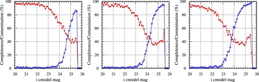
Fractions of the ACS stellar objects classified as stellar in the HSC stellar selection (red filled circles connected with solid line), and of the ACS extended objects contaminating among the HSC stellar objects as a function of i-band magnitude (blue open circles connected with solid line). Left: Based on the stack simulating the best seeing conditions with FWHM = 0|${^{\prime\prime}_{.}}$|5. Middle: Simulating the median seeing conditions with FWHM = 0|${^{\prime\prime}_{.}}$|7. Right: Bad seeing conditions with FWHM = 1|${^{\prime\prime}_{.}}$|0. It should be noted that i-band data in the Wide-layer are mostly taken under good and median seeing conditions. (Color online)
2.3 Color selection criteria for z ∼ 4 quasars
Candidate z ∼ 4 quasars are selected from stellar objects on the g − r vs. r − z color–color diagram. Figure 2 summarizes the distribution of the S16A-Wide2 stellar objects with known spectroscopic information on the color–color diagram. The selection criteria are determined with the aim of including as many quasars between 3.5 < z < 4.0 as possible, while minimizing the contamination by other objects. The determined selection criteria are shown with solid lines. They are
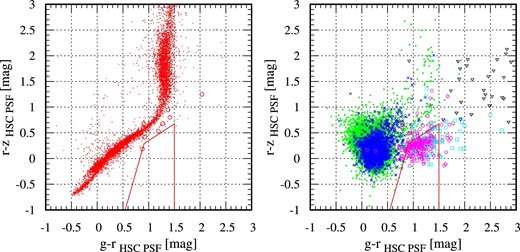
Distribution of HSC stellar objects with spectroscopic information on g − r vs. r − z color–color diagram. Left: Distributions of Galactic stars. Red dots represent Galactic stars; large red open circles represent HSC colors of Galactic stars identified in the z ∼ 4 quasar survey in the COSMOS region (Ikeda et al. 2011). Right: Distributions of extragalactic objects at five different redshift ranges: 0.5 < z < 2.5 (green dots), 2.5 < z < 3.5 (blue crosses), 3.5 < z < 4.0 (pink open circles), 4.0 < z < 4.5 (cyan open squares), 4.5 < z (black triangles). Red solid lines in both of the panels indicate the color selection criteria used in this paper. (Color online)
In order to constrain the quasar luminosity function at z ∼ 4 without conducting further spectroscopic follow-up observations, we set relatively tight color selection criteria to minimize contamination of red Galactic stars. For example, Ikeda et al. (2011) use wider selection criteria to select z ∼ 4 quasar candidates for spectroscopic follow-up observations in the COSMOS region, and they found a significant contamination by Galactic stars. The HSC colors of their Galactic stars are shown with open red circles in the left-hand panel of the figure. We set the tighter selection criteria of not including these stars by rejecting a non-negligible fraction of z ∼ 4 quasars with known spectroscopic redshift. The fraction of quasars missed in the color selection is accounted for in the statistical evaluation of the survey effective area, discussed in the next section.
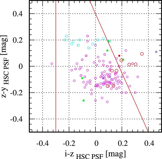
Distribution of HSC stellar objects with spectroscopic information on i − z vs. z − y color–color diagram. Symbols are the same as in figure 2. Only objects that meet the g − r vs. r − z color selection criteria are shown, except for Galactic stars identified in the z ∼ 4 quasar survey in the COSMOS region (Ikeda et al. 2011). Red solid lines indicate the color selection criteria used in this paper. (Color online)
After applying the stellarity and color criteria to the 20.0 < i < 24.0 objects which meet the flag conditions in table 2, we select 3227 candidate z ∼ 4 quasars. The number of candidates in each sub-region is summarized in the column Norg of table 1. However, if we check the five band images of the selected candidates, we find that junk objects contaminate the sample. Therefore, we apply further masking based on the mask image and the bright star catalogs as described below.
2.4 Additional masking and masking junk objects
In addition to the flags listed in the data base as shown in table 2, we further check similar flags in the mask images provided in the stacked image data base. The primary aim of this further masking process is to remove the junk objects. Additionally, we try to mimic the flag conditions shown in the table 2 simply, by constructing mock random objects uniformly distributed in the survey region, which is necessary in the evaluation of the effective survey area (see subsection 3.4). We mask objects which have the MP_EDGE, MP_BAD, MP_SAT, MP_NODATA, or MP_NOT_DEBLENDED flag within a radius of 5″ and MP_CR in the central 3 × 3 pixels. This masking is usually stricter than the flag cuts in table 2, therefore we only consider this masking in the process of generating the random mock objects.
The above flags and masking are not sufficient to remove objects with bad photometry in the catalog. For example, satellite tracks remaining in the stacked images can be cataloged as objects detected in one band. Such tracks themselves are not selected as a z ∼ 4 quasar candidates, but affect the photometry of real objects close to them. Ghost images and faint halos around bright stars can also be cataloged as objects meeting the above flag conditions, and also affect the photometry around them.
First, we remove objects around bright stars and galaxies. In the HSC catalog, objects around bright stars are flagged based on the Naval Observatory Merged Astrometric Data set (Zacharias et al. 2005). We remove objects that have the MP_BRIGHT_OBJECT flag within the radius of 5″ in the mask image. The process should mimic the flags_pixel_bright_object_any flag in the data base. In addition to the flag, we further consider bright objects cataloged in the Guide Star Catalog (GSC) version 2.3.2. We remove objects within rmask[″] = 150.0 from stars brighter than 10 mag, and rmask[″] = 20.0 + 17.1 × (13.5 − mag) from stars down to 15 mag. Among the multiple magnitudes available for one object in the GSC, we use the brightest magnitude of the object in the above calculation. The size of the additional masks are empirically determined by checking the distribution of “junk” objects around bright stars.
We also remove objects close to satellite tracks and faint halos around bright stars, because photometries of such objects are often unreliable. In the current data base, such satellite tracks and faint halos are detected as widely extended objects, and the pixels associated with them are flagged as MP_DETECTED in the mask image in the same way as for other real astronomical objects. We check the 10″ × 10″ region around each cataloged object and if more than 60% of the pixels around an object are flagged as MP_DETECTED in either of the five bands, the object is removed. Additionally, we examine the connected pixels around the object with this flag and if the total number of the connected pixels is more than 30% of the 10″ × 10″ pixels, we also mask the object. Furthermore, if the number of detected pixels in the i band is 2.0× larger than that in either of the r or z band, or those in the g, r, z, y bands are 2.0× larger than the i band, we mask the object. The size and fraction of the mask are determined by checking objects around remaining satellite tracks and faint halos.
The deblending process of the HSC pipeline does not provide reliable photometry for faint objects in the outskirts of relatively bright galaxies (i < 21). The above masks around very bright objects are not sufficient to remove such faint objects around bright galaxies. Therefore, we remove objects around stars and galaxies brighter than i < 22.0 mag. The radius of the mask, rmask, is determined with the adaptive moment of the object with |$r_{\rm mask}=1.8 \sqrt{\rm i\_hsm\_moment\_11}$|. In order to recover real candidates with i < 22.0 mag, we only consider the mask for objects fainter than i > 22.0 mag.
In the selection process, we apply all of the above additional masking processes after selecting 3227 candidate z ∼ 4 quasars with the stellarity and color selections described above. Once we apply the above masking processes, there are 1668 candidates left. The number in each sub-region is summarized in table 1. We check the selected candidates by eye, and confirm almost all of the junk objects and objects in the outskirts of bright objects are removed. We do not apply a junk object removal with the eyeball check. The same masking processes are also applied to random mock objects described in subsection 3.4 to mimic the object detection process.
2.5 Comparison with the z > 3 SDSS quasar selection
In order to compare the sample of the z ∼ 4 quasars based on the HSC Wide-layer photometric data with the spectroscopically identified quasars in the SDSS survey, we plot the size, color, and magnitude distributions of the 534 quasars at z = 3.0–4.5 from the spectroscopic data base of the 12th data release (DR12) of the SDSS (Alam et al. 2015) in the S16A-Wide2 coverage in figure 4. They are within the coverage and neither masked nor flagged by the masking process described in subsections 2.1 and 2.4, except for the HSC i < 22 mask. Red open and blue filled circles represent quasars which are recovered and missed in the above selection, respectively, with the photometric data of the HSC.

Top left: zspec vs. adaptive moment ratio of the SDSS quasars in the S16A-Wide2 coverage. Red open and blue filled circles represent SDSS quasars selected and missed by our HSC z ∼ 4 quasar selection criteria, respectively. The blue solid line indicates the criteria for stellar object selection. Top right: i-band magnitude vs. g − r color of the 534 SDSS quasars at z = 3.0–4.5. The magnitudes and colors are based on the SDSS photometry converted to the HSC system with the conversion discussed in subsection 3.3. Objects brighter than i < 20.0 mag are not selected by the HSC selection due to the effect of the saturation or non-linearity. Bottom left: zspec vs. g − r color of the 379 SDSS quasars fainter than i > 20.0 mag. Bottom right: zspec vs. r − z color of the 379 SDSS quasars fainter than i > 20.0 mag. (Color online)
The top left-hand panel of figure 4 shows the distribution of the adaptive moment ratio of the SDSS z > 3 quasars as a function of redshift. Most of the SDSS z > 3 quasars have an adaptive moment ratio consistent with the stellar object selection discussed in subsection 2.2 in the HSC Wide-layer image size and depth. Stellar morphological selection of quasars with deep imaging data can miss significant fraction of low-luminosity quasars due to their host galaxy contribution (Palanque-Delabrouille et al. 2013), however such an effect is negligible in the current data set for the SDSS z > 3 quasars.
In the top right-hand panel of figure 4, we show the distribution of g − r colors of the SDSS z > 3 quasars as a function of i-band magnitudes. Because the bright end of the sample can be affected by saturation or non-linearity, the top right-hand and bottom panels of figure 4 are plotted with the colors in the SDSS photometry converted to the HSC system using the conversion method discussed in subsection 3.3. Quasars with red g − r colors should be selected with the color selection, but they are missed above around i < 19.8 mag. Although in this plot we remove objects which have saturated pixels at the central 3 × 3 pixels by the saturation flag discussed in subsection 2.1, still some bright i < 20.0 mag stellar objects seem to be affected by saturation or non-linearity effects. Therefore, we limit the sample fainter than >20.0 mag in all of the r, i, z, and y bands, as mentioned above. There are 379 objects fainter than i > 20.0 mag among the 534 objects.
In the bottom left- and right-hand panels of the figure, we plot the g − r and r − z colors as a function of spectroscopic redshift for the 379 SDSS quasars, respectively. The g − r color of the quasars at z > 3.5 are red, and most of them are selected by the above color selection criteria; 92 quasars are above z = 3.5 and 61 are selected by the above z ∼ 4 quasar selections, i.e., 66% of the SDSS quasars are selected. Among the 31 missed quasars, one object is rejected by the stellarity criteria, 26 objects fail the g − r vs. r − z color selection, and four objects fail the i − z vs. z − y color–color selection.
2.6 Comparison with the X-ray selected z > 3 AGN samples
The blue color and stellar morphology selection of quasars is biased against obscured and/or less-luminous AGNs, because obscured and/or less-luminous AGNs can have extended morphology dominated by their host galaxy and/or red UV color due to the dust extinction. They can be missed in our selection criteria. X-ray selection of AGNs is one effective method to construct a sample of AGNs with little bias against obscured and/or less-luminous AGNs. In order to evaluate the bias associated with the stellarity and color selection, we examine distributions of stellarity and color of X-ray selected AGNs at z > 3 in the HSC Wide-layer data set.
We construct a sample of z > 3 X-ray selected AGNs by matching the HSC Wide-layer catalog with optical identification results in the X-ray survey of Subaru XMM-Newton Deep Survey (SXDS: Hiroi et al. 2012), XMM Large Scale Structure survey (XMM-LSS: Melnyk et al. 2013), XMM-XXL (Menzel et al. 2016), and AEGIS-X Deep (AEGIS-XD: Nandra et al. 2015) regions covered in the Wide-layer data set. We also include z > 3 X-ray selected AGNs in the COSMOS region (Vito et al. 2014: Marchesi et al. 2016a) by using the simulated stacked images of the Wide-layer depth under the median seeing condition (see subsection 2.2). After excluding overlapping identifications, there are 130 z > 3 X-ray AGNs matched with HSC sources in the magnitude range of iPSF = 20.0–24.0 mag. In order not to be biased toward stellar AGNs, we include AGNs with a photometric redshift. It should be noted that the combined sample is not statistically complete; the sample consists of AGNs selected in the surveys with various X-ray flux limits and areas.
The top left- and right-hand panels of figure 5 show the distribution of the adaptive moment ratio as a function of redshift and i-band magnitude, respectively. Red open and blue filled circles represent the z > 3 X-ray AGNs which are recovered and missed in the HSC z ∼ 4 quasar selection, respectively. Most of the X-ray selected AGNs at z > 3.6 have stellar morphology, thus at a face value the stellarity selection seems not to miss a significant fraction of X-ray selected AGNs in this redshift range. However, the fraction of stellar objects among the z > 3 AGNs show strong dependence on magnitude; 88% (65 out of 74) of z > 3 X-ray AGNs brighter than i = 22.5 mag are unresolved, but only 32% (18 out of 56) z > 3 X-ray AGNs fainter than i = 22.5 mag have stellar morphology. It is suggested that the stellarity selection can miss a significant part of AGNs fainter than i = 22.5 mag due to the host galaxy contamination. The magnitude corresponds to a quasar with M1450 ∼ −23.5 mag at z = 4. The bottom left- and right-hand panels show the g − r and r − z colors of the z > 3 AGNs; z ∼ 4 X-ray selected AGNs cover a similar color range to the SDSS quasars. Thus the g-dropout selection will not introduce severe bias against obscured AGNs. Further statistical discussion based on the comparison with the X-ray luminosity function of AGNs will be made in subsection 5.3.
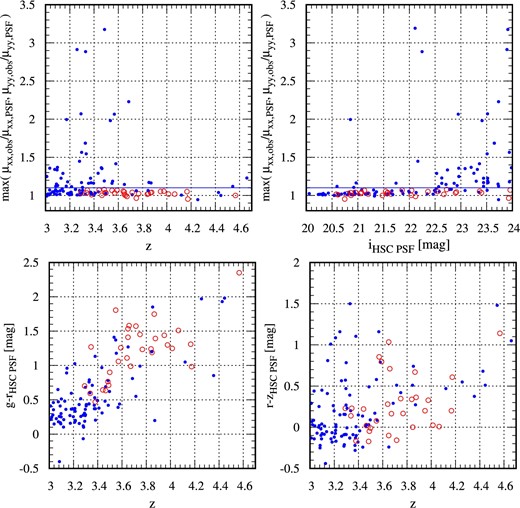
Top-left: z vs. adaptive moment ratio of the X-ray selected AGNs at z > 3.0 with i = 20.0–24.0 in the Wide-layer data set (see text for details). Red open and blue filled circles represent X-ray AGNs selected and missed by our HSC z ∼ 4 quasar selection criteria, respectively. The blue solid line indicates the criteria for stellar object selection. Top right: i mag vs. adaptive moment ratio of the X-ray selected AGNs at z = 3.0–4.5. X-ray selected AGNs with i > 22 mag show significantly extended morphology in the Wide-layer data set. Bottom left: z vs. g − r color of the X-ray selected AGNs. Bottom right: z vs. r − z color of the X-ray selected AGNs. (Color online)
3 z ∼ 4 quasar number counts
3.1 Modeling photometric uncertainty at each position
In order to derive the number counts of the z ∼ 4 quasar sample, we evaluate the effective survey area of the S16A-Wide2 data set for the quasars as a function of magnitude and redshift. We consider the variation of the depth of the images due to the variation of seeing and atmospheric transparency conditions and the number of available raw frames at each location.
The depth at each position is represented by the photometric uncertainty, which is estimated with the variance images of the stacked images. The photometric uncertainties of real objects correlate well with the variance values at the object positions. The correlation shows the dependence on the size of the object, i.e., extended objects have larger photometric uncertainty than stellar objects at the same magnitude. Therefore, we construct equations to calculate photometric uncertainties for a given magnitude based on the model PSF size and the variance at each position. In this uncertainty model, it is assumed that the photometric uncertainty is dominated by the background noise and is not affected by the object Poisson noise. In reality the objects at the detection limits are faint enough to meet the assumption.
The effective survey area is evaluated as follows. First, we construct libraries of quasar photometric models. Then, we randomly locate the quasar models within the survey region, and add random photometric error evaluated with the variance value at the random position as described above. Finally, we apply the same magnitude and color selection to the random quasar models and evaluate the effective survey area using the ratio of recovered z ∼ 4 quasar models to total input models at each redshift and magnitude. Details of the process are described in the next three subsections.
3.2 Constructing a library of quasar photometric models with templates
The quasar photometric models are constructed based on a library of SEDs of z ∼ 4 quasars, which describes the distribution of the SEDs of broad-line quasar populations. We make a library of quasar SEDs considering the scatter of the power-law slope, the broad-line equivalent width (EW), and strength of absorption by the intergalactic medium (IGM). We assume quasar SEDs depend on luminosity, but do not depend on redshift.
The library of the quasar SEDs is constructed in the same way as described in Niida et al. (2016). The underlying power-law component, fν ∝ να, is modeled using three components covering different wavelength ranges. Below 1100 Å, we use α of −1.76 following Telfer et al. (2002). We apply α values of −0.46 and −1.58 between 1100 Å and 5011 Å and above 5011 Å, respectively, following Vanden Berk et al. (2001). For the slopes of two power-law components below 1100 Å and between 1100 Å and 5011 Å, we assume both of the slopes have a scatter with standard deviation of 0.30 around the average α, following Francis (1996).
The strength of emission lines is modeled relative to the C iv emission line following the emission line ratios tabulated in Vanden Berk et al. (2001). The strength of the C iv emission line is modeled by considering the dependence of the EW on quasar luminosity; the so-called Baldwin effect. We do not consider the luminosity dependence of the emission line ratios. The average and standard deviation of the C iv emission line’s EW are measured as a function of luminosity from quasar spectra of the Baryon Oscillation Spectroscopic Survey (BOSS) in the SDSS III. The measurement covers a luminosity range of M1450 = −21.5 mag to −29.5 mag with 1 mag bin (Niida et al. 2016). No correction for a contamination by a host galaxy component is made. In addition to the isolated emission lines, the Fe ii multiplet emission features and Balmer continuum are added by using the template in Kawara et al. (1996).
Finally, we apply the effect of the absorption by the IGM. We use the updated number density of a Lyα absorption system in Inoue et al. (2014). We also consider the scatter of the number density via a Monte Carlo method described in Inoue and Iwata (2008).
We construct 1000 quasar SEDs in each magnitude bin from M1450 = −21.5 mag to −29.5 mag. Therefore, a total of 8000 quasar SEDs are constructed. Each spectrum is redshifted, and converted to observed flux. In figure 6, averages and 1σ scatters of the g − r and r − z colors of the model quasars are shown as a function of redshift. In the plot, we only consider model quasars with apparent magnitude between i = 20.0 to 22.0 mag. Green dots in the figure represent the colors of the SDSS DR12 quasars in the same magnitude range. The model quasars reproduce the distribution of the SDSS DR12 quasars. In figure 7, the distributions of the model quasars with magnitude between i = 20.0 and 22.0 mag in the redshift ranges z = 2.5–3.0 and z = 3.5–4.3 are plotted with contours in the left- and right-hand panels, respectively. The contours enclose 30%, 60%, 90% of the models in the redshift range from top to bottom. The distributions are compared to those of the SDSS DR12 quasars which are in the same magnitude range.
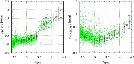
Distribution of the model quasars in the color vs. redshift plane compared to SDSS quasars with i = 20–22 mag within the S16A-Wide2 coverage. For a description of the model, see subsection 3.2. Left- and right-hand panels are for g − r and r − z colors, respectively. Open squares with error bars indicate the average and 1σ scatter of the model quasar color at each dz = 0.1 bin. Green points indicate colors of each SDSS quasar. In order not to be affected by the difference in the absolute magnitude, only model quasars in the same magnitude range are plotted. (Color online)
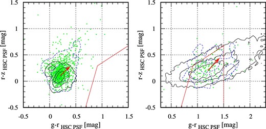
Distribution of the model quasars in the g − r vs. r − z color–color plane (solid contour) compared to SDSS quasars with i = 20–22 mag within the S16A-Wide2 coverage. For a description of the model, see subsection 3.2. Green points indicate colors of each SDSS quasar, and dashed contours show the distribution. Left- and right-hand panels are for quasars at z = 2.5–3.0 and z = 3.5–4.3, respectively. There are 1407 and 234 SDSS DR12 quasars in the redshift and magnitude ranges in the S16A-Wide2 coverage. In order not to be affected by the difference in the absolute magnitude, only model quasars in the same magnitude range are plotted. The contours represent 30%, 60%, and 90% enclosing areas. Red arrows indicate the effect of SMC-like dust-extinction with E(B − V) = 0.04 mag. Red solid lines represent the z ∼ 4 quasar selection criteria on the plane. It should be noted that the photometric uncertainty of the HSC is negligible for objects brighter than the SDSS spectroscopy. (Color online)
The 60% enclosing contour of the SED library reproduces that of the SDSS z = 2.5–3.0 quasars. However, the 90% enclosing contour of the SDSS z = 2.5–3.0 quasars shows extended distribution toward red r − z color. Reddening of the quasar spectrum by dust associated with the quasar can explain the extended distribution. The direction of the extension is consistent with the reddening vector with Small Magellanic Cloud-like dust extinction; the red arrows in the figure show the reddening vector with E(B − V) = 0.04 mag. The extended distribution that only appears in the 90% enclosing contour is broadly consistent with the fraction of reddened quasars in the SDSS sample. Richards et al. (2003) report 6% of SDSS quasars show red color, which is explained by E(B − V) larger than 0.04 mag. After correcting for the bias against reddened quasars, they estimate a total contribution of such dust-reddened broad-line quasars in the total quasar population of 15%. It should be noted that the fraction at the depth of the HSC Wide-layer can be higher. The fraction of missed AGNs due to obscuration is discussed in subsection 2.6.
In the current SED library, we do not include a population of quasars with dust reddening, primarily because current quasar samples at higher redshifts do not cover such a population (e.g., Richards et al. 2006; Ross et al. 2013; McGreer et al. 2013). In the higher redshift range, z = 3.5–4.3, the r − z color distribution of the SDSS quasars is well reproduced by the distribution of the quasar SED library. That means the current sample of z = 3.5–4.3 SDSS quasars does not include the reddened quasar population seen at z < 3 or that the fraction of such reddened quasars is really decreasing. In the current photometric sample, it is hard to tackle such reddened quasar populations due to heavy contamination by Galactic stars. We will need future wide-field multi-wavelength surveys to pick up the population.
On the other hand, the g − r color distribution of the SDSS quasars is narrower than that of the model quasars. The g − r color distribution in this redshift range is mostly determined by the strength and scatter of the IGM absorption. Currently, the number of z = 3.5–4.3 SDSS quasars covered by HSC photometry is rather limited to quantitatively determine the range of the color distribution, therefore we use the color distribution of the model quasars as a baseline sample of the full quasar population in this paper. Hereafter, we refer to the library of the quasar models as the library of quasar photometric models with templates.
It should be noted that the quasar SED library is constructed over a wide luminosity range using the spectra of less-luminous quasars at lower redshifts, assuming that the spectral shapes of the quasars do depend on luminosity but do not depend on redshift. Therefore, the library extends to a fainter luminosity range than the SDSS sample at z = 4 and is therefore applicable in this HSC study.
3.3 Quasar photometric models with a SDSS photometric sample
The other library of quasar photometric models is constructed by converting quasar PSF photometry from the SDSS DR12 quasar catalog into the HSC photometric system. Because the HSC survey area is not wide enough to cover large numbers of SDSS quasars at high-redshifts, and quasars brighter than i < 20.0 mag are affected by saturation in the HSC photometry, we construct a library of model quasars by converting SDSS photometry to HSC photometry instead of directly using the HSC photometry of the SDSS quasars.
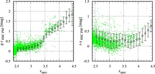
Distribution of the quasar photometric models with SDSS photometry in the color vs. redshift plane compared to SDSS quasars with i = 20–22 mag within the S16A-Wide2 coverage. For a description of the quasar photometric models, see subsection 3.3. Left- and right-hand panels are for g − r and r − z colors, respectively. Open squares with error bars indicate the average and 1σ scatter of the model quasar color at each dz = 0.1 bin. Green points indicate colors of each SDSS quasar. (Color online)
In figure 9, we compare the distribution of the model quasars with SDSS photometry at z = 2.5–3.0 and z = 3.5–4.3 with that of the SDSS quasars observed by the HSC system in the magnitude range i = 20–22 mag. The distribution of the converted photometry is broadly consistent with the HSC colors of SDSS quasars directly measured in the HSC images. For quasars at z = 2.5–3.0, the g − r colors of the quasars with red r − z colors show systematically bluer distribution. Hereafter, we refer to the library as the library of quasar photometric models with SDSS photometry.
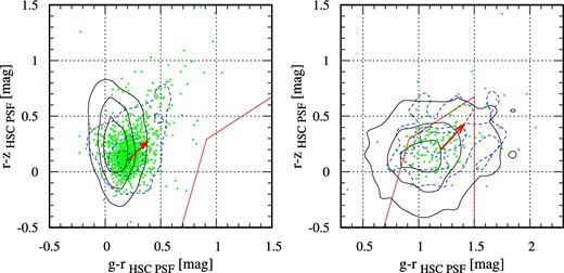
Distribution of the quasar photometric models with SDSS photometry in the g − r vs. r − z color–color plane is shown with the solid contour. For a description of the quasar photometric models, see subsection 3.3. SDSS photometry is converted to the HSC system. Green points indicate HSC colors of SDSS quasars with i = 20–22 mag within the S16A-Wide2 coverage, with the dashed contour showing their distribution. Left- and right-hand panels are for quasars at z = 2.5–3.0 and z = 3.5–4.3, respectively. There are 43123 and 4522 quasars in the redshift and magnitude ranges in the SDSS DR12 quasar catalog. The contours represent 30%, 60%, and 90% enclosing areas. Red arrows indicate the effect of SMC-like dust-extinction with E(B − V) = 0.04 mag. Red solid lines represent the z ∼ 4 quasar selection criteria on the plane. (Color online)
3.4 Estimating survey area as a function of redshifts and magnitudes
The effective survey area is determined as a function of magnitude and redshift for the quasar sample. We consider the effective survey area including the redshift selection function of the color selection. We use the above two libraries of quasar models to derive the effective survey area correcting the fraction of missed quasars among the “complete” sample. In order to derive the survey area at a certain magnitude limit, first random positions are selected within the survey region and then we apply the same masking processes described in subsection 2.4. We pick up 6000 random positions per deg2. The concept of the random positions is the same as is available in the data base as random objects (Aihara et al. 2018b). Secondly, we randomly assign one quasar model from one of the libraries. For the quasar models with template, we randomly draw a quasar model in the considered magnitude range, and for the quasar models with SDSS photometry, we randomly select one quasar, and normalize the SED to match the considered magnitude. Therefore, in the calculation with the quasar models with SDSS photometry, we ignore the luminosity dependence of the quasar SEDs. Then, we calculate uncertainties associated with the photometry in each band and we apply random fluctuations to the photometric model. Finally, we apply the magnitude (20.0 < i < 24.0) and color selection criteria to examine the fraction of recovered objects at the magnitude.
The resulting effective survey areas as a function of redshift at each magnitude are shown in figure 10. The left- and right-hand panels show the effective areas estimated with the quasar models with templates and those with SDSS photometry, respectively. They are broadly consistent with each other, though the area derived using the models with templates shows a broader redshift distribution than that which used the models with SDSS photometry as expected from the color distributions shown in figure 7. Both areas show a break at i = 22.0 mag, caused by the mask around objects with i < 22.0 mag. The peak of the survey area is 133.0 deg2 for i = 21.4 mag quasars at z = 3.65. In table 1, effective areas after removing masked regions are summarized. The effective areas are calculated applying the same masking process described in subsection 2.4. For the sixth and seventh columns, the areas without and with the masks with objects brighter than i < 22 mag, respectively, are shown. The total effective survey area for i < 22 mag objects is 172.0 deg2. The effective area for z ∼ 4 quasars includes the color selection efficiency of the quasars at each redshift as well as the effect of the masked regions and shallow areas. The peak of the survey area for z ∼ 4 quasars is 77% of the total effective survey area for i < 22 mag objects. The fraction is broadly consistent with the fraction of z > 3.5 SDSS quasars meeting the z ∼ 4 quasar selection criteria (66%), as discussed in subsection 2.3.
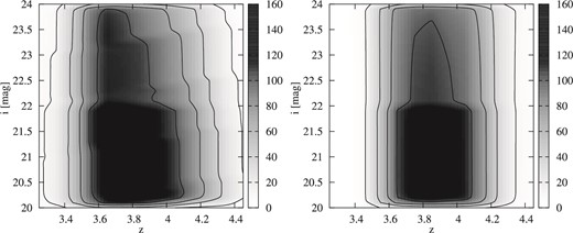
Survey area as a function of redshift and i-band magnitude. Left: Derived with the quasar templates. Right: Derived with the SDSS quasar photometry. The contours are plotted at 10 deg2, 40 deg2, 70 deg2, 100 deg2, and 130 deg2.
The differential number counts of the z ∼ 4 quasars are shown in figure 11 and summarized in table 3. The second and third columns show the raw number and surface number density of the quasars, respectively. We apply the average effective survey area between z = 3.6–3.8, where the color selection efficiency is maximized. In the number counts, we correct for the completeness of the stellarity selection assuming the median condition in figure 1. We do not correct for the contamination by the extended objects, because we consider the contamination in the next subsection. The number counts show a steady increase toward the faint-end, and excess at magnitudes fainter than i > 23.0 mag. We also examine the number counts in each sub-region. The results are shown with open squares with error bars estimated with the Poisson statistics. The number counts are consistent with those derived in the entire region, and the effect of the cosmic variance seems to be small, thanks to the large survey area. The scatter at the brightest end is large due to the limited number of the samples.
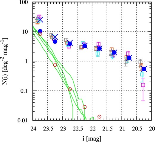
Differential number counts of z ∼ 4 quasar candidates. Blue crosses represent the number counts derived in the entire S16A-Wide2 region. Open squares are the number counts after dividing the region into the four sub-regions (pink: WideA, cyan: WideB, orange: WideC, and gray: WideD). The uncertainties associated with the number count in each sub-region are determined with the Poisson statistics. The open squares in each sub-region are shifted in horizontal direction for clarity. The filled circles show the number counts after correcting for the expected contamination by Galactic stars (green solid line for each sub-region) and the compact galaxies (red open circles). (Color online)
Number count of the z ∼ 4 quasars.
| i | N obs | n | n corr |
|---|---|---|---|
| (mag) | (deg−2 mag−1) | (deg−2 mag−1) | |
| 20.00–20.50 | 34 | 5.50 × 10⁻¹ | 5.48 × 10⁻¹ |
| 20.50–21.00 | 78 | 1.30 × 100 | 1.30 × 100 |
| 21.00–21.50 | 121 | 1.97 × 100 | 1.97 × 100 |
| 21.50–22.00 | 162 | 2.70 × 100 | 2.69 × 100 |
| 22.00–22.50 | 170 | 3.35 × 100 | 3.31 × 100 |
| 22.50–23.00 | 189 | 4.17 × 100 | 3.88 × 100 |
| 23.00–23.50 | 258 | 6.65 × 100 | 4.62 × 100 |
| 23.50–24.00 | 656 | 2.54 × 101 | 1.03 × 101 |
3.5 Contamination by extended objects
The expected contamination from extended objects that meet the z ∼ 4 quasar color selection criteria is evaluated. In addition to the Lyman Break Galaxies (LBGs) at z ∼ 4, foreground z < 1 galaxies can be contaminants to the z ∼ 4 quasar sample, because they can have similar colors to z ∼ 4 quasars due to their 4000 Å break.
Even with the ground-based HSC images, most of the z ∼ 4 LBGs are extended, thanks to the good image quality in the i band; thus only compact LBGs are contaminating the stellar object selection. In figure 12, the distribution of the measured adaptive moment ratios in the S16A-Wide2 data set of the 306 z > 3 and i > 23 galaxies that are spectroscopically identified in deep surveys is shown. Broad-line AGNs are removed in this plot. The red line indicates the selection criteria of the stellar objects. Thanks to the good image quality of the i-band image of the Wide-layer data set, the z > 3 galaxies are significantly extended compared to the stellar objects. The fraction of the galaxies that are classified as stellar is 6%. The fraction is larger than that observed among all galaxies with i = 24 mag (2%); in this evaluation we use the distribution of all galaxies in each magnitude range, because it is possible that the spectroscopically identified sample can be biased toward compact galaxies, and we do not know the true size distribution of z > 3 galaxies.
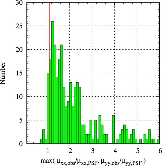
Distribution of the measured adaptive moment ratios of the 306 z > 3 i > 23 galaxies with spectroscopic identification. The red solid line indicates the selection criteria for stellar objects. (Color online)
At first, we construct a catalog of extended objects that meet the color criteria from the HSC-SSP S16A-Wide2 data base. This sample should contain not only z ∼ 4 LBGs, but also z < 1 galaxies that are contaminating the LBG selection. Then, we apply the masking processes described above. The number counts of the objects that are not masked in the process are calculated with the same survey area used for the z ∼ 4 quasar number count. The number count of extended objects that cause contamination is calculated by multiplying the fraction of ACS extended objects classified as stellar in HSC criteria as a function of magnitude. The fraction is determined in the same way as described in subsection 2.2, but this time the fraction of HSC stellar objects among the ACS extended objects is calculated. We use the results with the median condition. In this calculation, we assume that the contaminating extended galaxies have the same size distribution as the entire galaxies in the same magnitude range. The resulting contamination by extended objects is shown with red open circles in figure 11. The estimated result suggests that contamination by extended objects can contribute to the number counts below i = 23.5 mag, and one third of the z ∼ 4 quasar candidates in the i = 23.5–24.0 mag bin can be a result of contamination by extended objects, which are non-AGN galaxies. The estimation is consistent with the rapid increase in the contamination by extended objects shown in figure 1.
3.6 Contamination by Galactic stars
The contamination by Galactic stars is evaluated by multiplying the observed number counts of Galactic stars in each sub-region with the fraction of Galactic stars meeting the z ∼ 4 quasar color selection criteria evaluated as a function of i-band magnitude. Both of the number counts and the fraction are estimated with a photometric library of Galactic stars in the HSC system.
A photometric library of Galactic stars is constructed as follows. At first, we collect a list of spectroscopically identified Galactic stars in the S16A-Wide2 data base which are flagged and masked in the same way as described in subsections 2.1 and 2.4. Then, we remove some outliers, which are outside of the stellar sequence seen in the g − r vs. r − z color–color diagram. The distribution of resulting stars on the color–color diagram is shown in figure 13 with red dots. This list of stars covers a wide range of stellar types. However, they can have a different mixture of types from that at the HSC Wide-layer depth because most of the spectroscopic identifications are from the SDSS DR12 data base, the depth of which is shallower. Therefore, we match the list of flagged and masked stellar objects in the S16A-Wide2 data base with the above list of the spectroscopically identified Galactic stars on the g − r vs. r − z color–color diagram, based on the distance in the diagram, rcol, being less than 0.1 mag. The distribution of resulting stars are shown in the figure using gray scale. It follows the distribution of the spectroscopically identified stars, but is more heavily populated with late-type stars compared to that of the spectroscopically identified stars. Open green circles indicate the colors of stars in the spectrophotometric library of Gunn and Stryker (1983). The circles show a systematic offset from the observed sequence of the late type stars redder than r − z > 1.0. The difference in the stellar metallicity is thought to be the cause of the systematic offset (Fukugita et al. 2011).
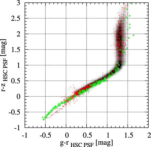
g − r vs. r − z color–color distribution of Galactic stars. Red dots indicate the spectroscopically identified Galactic stars in the S16A-Wide2 data base (a randomly selected 30% of stars are plotted for clarity), and the gray scale represents the distribution of the stellar objects in the S16A-Wide2 data base which are selected based on the distance on the diagram, rcol < 0.1 mag, from red dots. Green dots indicate colors of Gunn–Stryker stars (Gunn & Stryker 1983) in the HSC system. (Color online)
Then, the number counts of Galactic stars are derived in the same way as for the z ∼ 4 quasars. First, we apply the masking process described in subsections 2.1 and 2.4 to the list of stellar objects in the HSC data base. Then the area of survey region is determined by random model objects constructed from a photometric library of Galactic stars. We assume that the photometric error in the photometric library is negligible, because we only consider stars which have similar colors to the bright, spectroscopically identified stars with negligible photometric errors. Then, we add a random photometric error predicted at each location in the same way described in subsection 3.4 and pick up random objects above the detection limit, i.e., i < 24.0 mag and the predicted photometric errors in i and z bands are smaller than 0.1 mag. The resulting number counts are shown in figure 14. The raw number counts in each sub-region are shown by a thin blue line. Sub-region WideA shows smaller number counts than the other three regions in the magnitude range i < 23 mag, and the solid line is located lower than the other three lines. In order to derive the intrinsic number counts of Galactic stars, we correct for the completeness and contamination of the star–galaxy separation by applying the fraction shown in figure 1. The resulting number count after the corrections are shown by thick red lines. The number count shows steady increase toward i = 22–24 mag, but then shows a plateau or decline towards the faint-end.
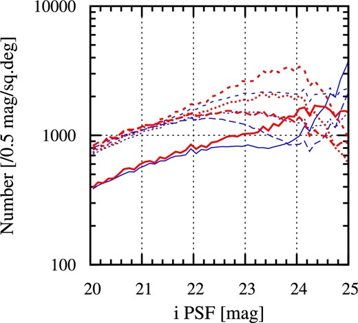
Differential number counts of Galactic stars in the four sub-regions (solid, dotted, dashed, and long-dashed lines represent WideA, WideB, WideC, and WideD sub-regions, respectively). Blue thin lines show raw count, and red thick lines represent after-correcting for contamination by extended galaxies following the contamination rate shown in figure 1. (Color online)
The expected contamination rate in the quasar number counts in each sub-region is shown in figure 11 by the green solid lines. Because photometric uncertainty increases toward fainter objects, the expected contamination of Galactic stars increases rapidly, although the number counts themselves show plateau at i = 22–24 mag. The expected number of contaminations varies in the four sub-regions depending on the distance from Galactic plane. The contamination by Galactic stars can contribute one third of the number counts in the i = 23.5–24.0 and i = 23.0–23.5 mag bins.
3.7 Number counts after correcting for the contamination
Based on the estimated number counts for the contamination, we evaluate the contamination rate, which is the fraction of contaminating objects among the candidates of z ∼ 4 quasars. For the contamination by Galactic stars, where the expected number depends on the Galactic coordinate of a sub-region, we average the number after weighting the survey area of each sub-region. The resulting contamination rate in each i-band magnitude bin is shown in figure 15 with crosses. In the magnitude range fainter than i > 23.5 mag, the contamination rate is estimated to be higher than 50%. In order to correct for the contamination statistically, we fitted the contamination rate with the error function. The best-fitting function is derived as pcont = erfc[ − 1.15(i − 23.59)]/2, and plotted as solid line in figure 15.
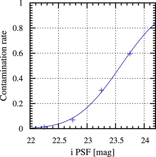
Contamination rate of the z ∼ 4 quasar selection. Contamination by Galactic stars as well as compact LBGs are considered. The solid curve indicates the best-fitting model with the error function. (Color online)
We correct for the expected contamination by assigning weight for each object based on the probability of non-contamination, i.e., the contamination rate subtracted from 1. If the contamination rate is 0.8 at the magnitude of an object, we assign a weight of 0.2 for the object, and the weight is summed when we calculate the number count and the luminosity function. The total sum of the weight of 1666 candidates is 1155.2, i.e., one third of the sample can be contamination mostly contributing i > 23.5 mag. The number counts after correcting for the contamination are shown using blue filled circles in figure 11 and summarized in the fourth column of table 3. Once we correct for the contamination statistically, the number density shows a monotonic increase towards the faint-end. The excess seen in the magnitude range i > 23 mag can be explained by the contamination from Galactic stars and compact galaxies that meet the g-dropout selection.
4 Results
4.1 Redshifts and absolute magnitudes
Among the 1668 z ∼ 4 quasar candidates, 76 of them have spectroscopic redshift information in the literature. Most of the redshift identifications come from the SDSS quasar surveys. A few of them are from deeper surveys (e.g., Akiyama et al. 2015). Their redshift distribution ranges between 3.4 and 4.2, shown by the red histogram in figure 16. Two SDSS quasars that have redshift z ∼ 1 are contaminating the sample. The two quasars have g − r colors of 0.37 and 0.50 in the SDSS data base, while those in the HSC are 0.81 and 0.95. Because they are located within 34΄ of each other, their HSC photometry could be affected by an unknown photometric problem in that specific region.

Redshift distribution of the z ∼ 4 quasar candidates. Green and blue histograms show the distributions of candidates with i < 24.0 and 21.0 < i < 23.5, respectively. Red histograms indicate the redshift distribution of quasars with spectroscopic redshifts. (Color online)
The resulting photometric redshift is plotted against the spectroscopic redshift in figure 17. The derived photometric redshifts do not show catastrophic errors, and follow the range of the spectroscopic redshifts. If we remove two outliers whose spectroscopic redshifts are z ∼ 1, the average and σ of the difference between zphot and zspec are −0.007 and 0.143, respectively. The systematic offset between the zphot and zspec is negligible.
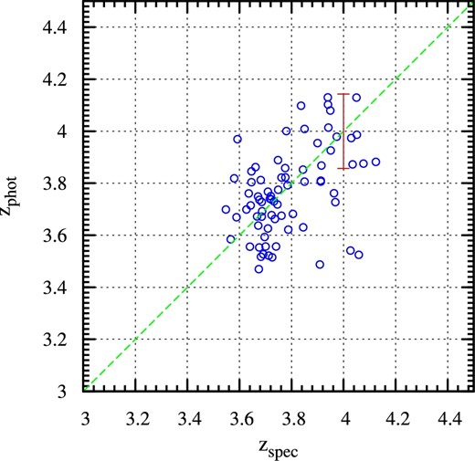
Photometric redshift vs. spectroscopic redshift. The green dashed line indicates the equality. The error bar indicates the σ of the difference between zspec and zphot. (Color online)
The distribution of the zphot and zspec is shown in figure 16 with a green histogram. Most of the selected quasars are distributed between z = 3.5 and 4.3. The range is consistent with the selection function evaluated in figure 10. The average of the redshift of the sample is 3.9. The redshift distribution of quasars in 21.0 < i < 23.5, which are less affected by contamination and are used in a clustering analysis (He et al. 2018), shows a similar distribution as the entire sample.
We derive M1450 either with zphot or zspec. M1450 is derived by interpolating the broad-band photometry around rest-frame 1450 Å. The uncertainty of M1450 associated with zphot is evaluated by the difference of M1450 with zspec and zphot for the 74 objects with zspec. The resulting σ of the difference is 0.082 mag. The estimated M1450 are plotted against redshift in figure 18 with red filled and blue open circles for objects with zspec and zphot. Most of the spectroscopically identified objects are from the SDSS catalog, and distributed in the magnitude range smaller than −24 mag.
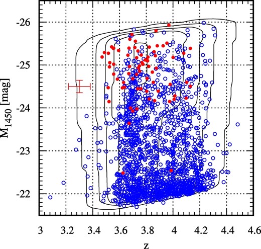
Estimated redshift and M1450 of the z ∼ 4 quasar candidates. Red filled and blue open circles represent quasars with spectroscopic and photometric redshifts, respectively. The error bar shows the uncertainty associated with the redshift and M1450 estimations. Contours represent the survey area at each redshift and M1450. The contours are plotted at 10 deg2, 40 deg2, 70 deg2, 100 deg2, and 130 deg2. (Color online)
4.2 Binned quasar luminosity function at z ∼ 4
The luminosity function of quasars at z ∼ 4 is calculated, using the photometric redshifts, M1450, and the survey area as a function of redshift and M1450. We evaluate the survey area again using the library of quasar models with templates. The resulting effective survey area as a function of redshift and M1450 is shown in gray scale in figure 19. We also plot the effective survey area using contours in figure 18. The distribution of the sample in the redshift-M1450 plane is consistent with that expected from the effective survey area. It should be noted that the effective survey area includes the efficiency of the quasar color selection, and the quasar models do not contain reddened quasar SEDs (see subsection 3.2).
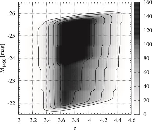
Effective survey area as a function of redshift and M1450. The contours are plotted at 10 deg2, 40 deg2, 70 deg2, 100 deg2, and 130 deg2. The effective survey area includes the efficiency of the color selection for the mock quasars. The upper and lower edges are determined with i > 20.0 and i < 24.0 mag selection criteria. The gap seen in the middle reflects the effect of the masks around HSC objects brighter than i < 22.0 mag. For objects brighter than i < 22.0 mag, the masks are not applied. The completeness of the stellar classification is not included in the calculation.
The resulting luminosity function is shown in figure 20 with red filled squares. Thanks to the wide and deep coverage of the HSC Wide-layer data set, the faint-end of the quasar luminosity function at z ∼ 4 is constrained with unprecedented accuracy, and the break of the luminosity function is clearly detected at around M1450 ∼ −25 mag. The binned luminosity function is shown in table 4. The uncertainty, σ, in each bin is determined with the Poisson statistics.
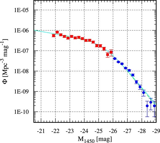
Luminosity function of z ∼ 4 quasars derived in this work. Red filled squares and blue filled circles represent results based on the HSC and SDSS DR7 quasar samples, respectively. Cyan solid and green dashed lines show the best-fitting double power-law model with the maximum likelihood fit to the sample and the χ2 fit to the binned luminosity functions. (Color online)
Binned z ∼ 4 quasar luminosity function.
| M 1450 | N corr | log (Φ) | σ |
|---|---|---|---|
| (mag) | (Mpc−3 mag−1) | (10−9 Mpc−3 mag−1) | |
| HSC S16A-Wide2 | |||
| −21.875 | 47.7 | −6.253 | 80.733 |
| −22.125 | 129.0 | −6.088 | 71.892 |
| −22.375 | 103.7 | −6.219 | 59.367 |
| −22.625 | 92.8 | −6.298 | 52.208 |
| −22.875 | 78.5 | −6.382 | 46.855 |
| −23.125 | 95.8 | −6.297 | 51.538 |
| −23.375 | 81.4 | −6.369 | 47.366 |
| −23.625 | 90.4 | −6.341 | 47.960 |
| −23.875 | 84.7 | −6.405 | 42.783 |
| −24.125 | 74.0 | −6.493 | 37.343 |
| −24.375 | 76.0 | −6.487 | 37.385 |
| −24.625 | 63.0 | −6.577 | 33.384 |
| −24.875 | 43.0 | −6.745 | 27.422 |
| −25.125 | 42.0 | −6.756 | 27.088 |
| −25.375 | 30.0 | −6.899 | 23.032 |
| −25.625 | 14.0 | −7.189 | 17.287 |
| −25.875 | 8.0 | −7.077 | 29.581 |
| SDSS DR7 z = 3.6–4.2 | |||
| −26.125 | 260.0 | −7.387 | 2.545 |
| −26.375 | 287.0 | −7.552 | 1.657 |
| −26.625 | 234.0 | −7.642 | 1.490 |
| −26.875 | 144.0 | −7.853 | 1.169 |
| −27.125 | 111.0 | −7.966 | 1.026 |
| −27.375 | 66.0 | −8.192 | 0.791 |
| −27.625 | 30.0 | −8.534 | 0.534 |
| −27.875 | 17.0 | −8.781 | 0.402 |
| −28.125 | 9.0 | −9.057 | 0.292 |
| −28.375 | 2.0 | −9.710 | 0.138 |
| −28.625 | 3.0 | −9.534 | 0.169 |
| −28.875 | 2.0 | −9.710 | 0.138 |
4.3 z ∼ 4 quasar sample from SDSS DR7
In order to construct the luminosity function covering a wide luminosity range based on quasars selected with consistent selection criteria, we combine z = 3.6 to 4.2 quasars from the spectroscopically identified quasar catalog from SDSS DR7 (Schneider et al. 2010). We use the DR7 catalog because it fully covers the SDSS legacy survey with a uniform color selection for high-redshift quasars. In the SDSS legacy survey, candidates of high-redshift quasars are selected with stellar morphology and multi-color selection for spectroscopic follow-up (Richards et al. 2002). A uniform target selection is applied for spectroscopy, except for the early phase of the SDSS survey. In order to construct a statistical sample, we only consider objects which are spectroscopically observed as science primary objects based on the final uniform target selection (objects with SCIENCEPRIMARY =1 and with “selected with the final quasar algorithm” =1 based on the TARGET photometry; see table 1 of Schneider et al. 2010). The effective survey area of the SDSS DR7 sample is determined to be 6248 deg2 by Shen and Kelly (2012).
The selection function of the uniform target selection is evaluated in Richards et al. (2006) as a function of redshift and magnitude. In the redshift range between z = 3.6 and 4.2, the SDSS target selection efficiency is estimated to be larger than 90%, mostly ∼100% (figure 6 of Richards et al. 2006). The target selection for high-redshift quasar is complete down to i < 20.2 mag, therefore we select 1260 quasars brighter than Mi(z = 2) < (z − 3.0) − 26.85 as a statistically complete sample in the above effective area (figure 17 of Richards et al. 2006). We assume that the sample is complete in the redshift range above the absolute magnitude limit. Utilizing the absolute magnitude limit as a function of redshift, we calculate the effective survey volume for each object with its Mi(z = 2). UV absolute magnitudes, M1450, of the quasars in the sample are derived from the broad-band SDSS photometry of the quasars in the same way as for the HSC z ∼ 4 quasars.
The resulting luminosity function is shown in figure 20 with blue filled circles and summarized in table 4. The second column indicates the number of the quasars in each absolute magnitude bin after correcting for the contamination rate. The luminosity function smoothly connects to the luminosity function determined with the HSC z ∼ 4 quasar candidates. Because the magnitude range of the HSC z ∼ 4 quasar candidates is fainter than i > 20.0 mag and the SDSS DR7 sample is i < 20.2 mag, there is no overlap in the bin of the luminosity function.
4.4 Double power-law model
Parameters of the best-fitting z ∼ 4 quasar luminosity function with a double power-law model.
| Method | Φ* | α | β | |$M_{1450}^{*}$| | Note |
|---|---|---|---|---|---|
| (1 × 10⁻⁷ Mpc−3 mag−1) | [Faint end] | [Bright end] | (mag) | ||
| Maximum Likelihood | 2.66 ± 0.05 | −1.30 ± 0.05 | −3.11 ± 0.07 | −25.36 ± 0.13 | Fitting to the sample |
| χ2 minimization | 2.41 ± 0.56 | −1.32 ± 0.08 | −3.18 ± 0.11 | −25.44 ± 0.19 | Fitting to the binned |
| luminosity function |
We also fit the binned luminosity function with a double power-law model through the χ2 minimization. The resulting best-fitting parameters are summarized in the second line of table 5 and the best-fitting function is shown in figure 20 as a green dashed line. The best-fitting parameters are consistent with each other.
5 Discussion
5.1 Comparison with previous results on the z ∼ 4 quasar luminosity function
The luminosity function derived in this work is compared with previous work in figure 21. In the bright-end, the binned luminosity function of z ∼ 4 SDSS DR7 quasar is fully consistent with those at z = 3.75, with the DR3 sample plotted with blue crosses (Richards et al. 2006) and the DR7 sample plotted with green open triangles (Shen & Kelly 2012). We convert Mi(z = 2) used in those papers to M1450 with M1450 = Mi(z = 2) + 1.486 (appendix B of Ross et al. 2013). Thanks to the larger effective area of the DR7 sample, the luminosity function from the DR7 sample extends to higher luminosities than the DR3 sample.
![Luminosity function of z ∼ 4 quasars derived in this work (red filled squares: HSC, and blue filled circles: SDSS DR7, with cyan solid and green dashed lines showing the best-fitting double power-law model same as in figure 20) compared with previous results [blue crosses: 3.5 < z < 4.0 luminosity function from SDSS DR3 (Richards et al. 2006), green open triangles: 3.5 < z < 4.0 luminosity function with SDSS DR7 quasar sample (Shen & Kelly 2012), blue open circles: 3.5 < z < 4.0 luminosity function derived with time-variability selection (Palanque-Delabrouille et al. 2013), pink open diamonds: 3.7 < z < 4.7 luminosity function derived from the COSMOS quasar survey (Niida et al. 2016), blue open squares: 3.5 < z < 5.0 luminosity function derived from the COSMOS quasar survey (Masters et al. 2012), red asterisks: 3.7 < z < 5.1 luminosity function derived from NDWFS (Glikman et al. 2011)]. For the last three luminosity functions, their normalizations are corrected by a factor of 1.2 to correct for the difference in the covered redshifts. Red pentagons show z = 4.0–4.5 X-ray-selected AGN luminosity functions from Giallongo et al. (2015). The normalization is corrected by a factor of 1.6. The blue dashed line is the best-fitting luminosity function from the COSMOS survey (Masters et al. 2012) after correcting for the normalization. (Color online)](https://oup.silverchair-cdn.com/oup/backfile/Content_public/Journal/pasj/70/SP1/10.1093_pasj_psx091/2/m_pasj_70_sp1_s34_f14.jpeg?Expires=1749170037&Signature=t-A7hSLIMUO7Ip68paGLGrzUiJnUB7xu62We5TFWW3a7hiSaqKFnRSnHOTvA4NmQ3g4dXScUtUC--M8evSipr~XfgKiHBdcdzm3lI~Ow9sEl-JrRR4HQHBmDMDdZhdq1kWetRVILChQtSHiGUZPcld2ZbIKu9AZmqWuIqBNOe9u9TjCmIRQPLSA7O16FJkLGeb0PrWynS0RpYykFVnsioAhqyP699W48th5WJOViiaNIVR5GrJo2ffjg~1q4vl0W8OxNmoZA3~CElSAT8jsUtrnFeOqp7x-mWXRfRPd8ZPnwXOevqNrzmt~-bJgiBd8~imFx-oJjrPoK3tLHPQxIHg__&Key-Pair-Id=APKAIE5G5CRDK6RD3PGA)
Luminosity function of z ∼ 4 quasars derived in this work (red filled squares: HSC, and blue filled circles: SDSS DR7, with cyan solid and green dashed lines showing the best-fitting double power-law model same as in figure 20) compared with previous results [blue crosses: 3.5 < z < 4.0 luminosity function from SDSS DR3 (Richards et al. 2006), green open triangles: 3.5 < z < 4.0 luminosity function with SDSS DR7 quasar sample (Shen & Kelly 2012), blue open circles: 3.5 < z < 4.0 luminosity function derived with time-variability selection (Palanque-Delabrouille et al. 2013), pink open diamonds: 3.7 < z < 4.7 luminosity function derived from the COSMOS quasar survey (Niida et al. 2016), blue open squares: 3.5 < z < 5.0 luminosity function derived from the COSMOS quasar survey (Masters et al. 2012), red asterisks: 3.7 < z < 5.1 luminosity function derived from NDWFS (Glikman et al. 2011)]. For the last three luminosity functions, their normalizations are corrected by a factor of 1.2 to correct for the difference in the covered redshifts. Red pentagons show z = 4.0–4.5 X-ray-selected AGN luminosity functions from Giallongo et al. (2015). The normalization is corrected by a factor of 1.6. The blue dashed line is the best-fitting luminosity function from the COSMOS survey (Masters et al. 2012) after correcting for the normalization. (Color online)
Around the knee of the luminosity function, Palanque-Delabrouille et al. (2013) evaluate the luminosity function based on a quasar sample selected by a variability selection. The luminosity function is described with Mg(z = 2) and we convert M1450 = Mg(z = 2) + 1.272 based on figure 12 of Palanque-Delabrouille et al. (2013). The binned luminosity function covering 3.5 < z < 4 is plotted with blue open circles in the figure. The binned luminosity function is fully consistent with the luminosity function of this work, within the uncertainty.
In Ikeda et al. (2011), Glikman et al. (2011), Masters et al. (2012), and Niida et al. (2016), the quasar luminosity functions are derived down to M1450 = −21 mag in deeper but narrower surveys than the SDSS. These functions are determined in the redshift ranges 3.7 < z < 4.7, 3.7 < z < 5.1, 3.5 < z < 5.0, and 3.7 < z < 4.7. They cover a redshift range that has a higher average redshift of the samples, z = 4.0, than the HSC sample (z = 3.9), therefore we compare with them after correcting for the evolution effect. In this redshift range, the number density of quasars evolves as (1 + z)−6.9 (Richards et al. 2006), and we correct for the difference by multiplying the averages of the samples by 1.2. The binned luminosity functions in the results are shown with pink open diamonds, red asterisks, and blue open squares for Niida et al. (2016), Glikman et al. (2011), and Masters et al. (2012) samples, respectively, in figure 21. The binned luminosity functions derived in the COSMOS regions (Niida et al. 2016; Masters et al. 2012) matches that of this work well, except for the faintest luminosity bin at M1450 = −21 mag. They select z ∼ 4 quasars with stellar morphology and a dropout selection method in a similar way to this study. On the other hand, the luminosity function in Glikman et al. (2011), based on the NOAO Deep Wide-Field Survey (NDWFS) data set, shows significantly higher number density than the other results. They use a similar selection method with dropout color and stellar morphology, but they use loose selection criteria for stellarity based on ground-based imaging data with a FWHM of 1″, and it would be possible that their sample is significantly contaminated by extended non-AGN objects below R > 22.5 mag (figure 4 in Glikman et al. 2010). It should be noted that the number density of LBGs rapidly increases below i > 23 mag, and they can not be distinguished from the quasars with the loose stellarity criteria.
Although the binned luminosity functions in the COSMOS regions are consistent with this work except for the faintest bin, the best-fitting luminosity function in Masters et al. (2012) has a much steeper slope than that in this work. The best-fitting luminosity function, after correcting for the redshift difference by multiplying by 1.2, is shown in figure 21 with a blue dashed line. The steeper slope is mostly caused by the excess number counts at M1450 = −21 mag, and cannot reproduce the luminosity function brighter than the knee. In subsection 5.3, we further discuss the difference in the best-fitting luminosity functions at z ∼ 4.
By integrating the best-fitting luminosity function, we estimate the UV luminosity density at 1450 Å of the quasars at z ∼ 4 to be ε1450 = 3.2 × 1024 erg s−1 Hz−1 Mpc−3, which is similar to that with the best-fitting luminosity function by Masters et al. (2012) (ε1450 = 3.1 × 1024 erg s−1 Hz−1 Mpc−3 after correcting for the evolution factor of 1.2). Giallongo et al. (2015) derive the UV luminosity function of X-ray selected AGNs and argue that the AGN emissivity of UV ionizing photons could be as high as the value required to keep the intergalactic medium highly ionized. Their UV luminosity function is shown with red pentagons in figure 21. We correct for the redshift evolution by multiplying their number density by 1.6, assuming the middle point of their redshift coverage (z = 4.0–4.5) and a number density evolution of (1 + z)−6.9. Their number density is more than one order of magnitude higher than the extrapolation of our best-fitting luminosity function at z ∼ 4. Their estimated UV luminosity density is 18.3 × 1024 erg s−1 Hz−1 Mpc−3 after correcting for the evolution factor. Our estimate is about six times smaller than their value. The difference could be caused by the bias of the optically selected stellar blue quasar sample against faint and/or obscured AGNs. In any case, the UV luminosity density of the best-fitting luminosity function of the HSC z ∼ 4 quasars suggests that the stellar blue quasars are not the main contributor to the cosmic reionization.
5.2 Evolution of the quasar luminosity function in the early universe
The evolutionary trend in the luminosity function of quasars above the peak of their number density at z ∼ 2 − 3 is a fundamental observable for understanding the early growth of SMBHs. In the left-hand panel of figure 22, the binned quasar luminosity function at z ∼ 4 is compared with those at z ∼ 2.3 (green open circles: Ross et al. 2013), z ∼ 2.7 (pink open pentagons: Ross et al. 2013), z ∼ 3.2 (blue open squares: Ross et al. 2013; blue open triangles: Masters et al. 2012), and z ∼ 5 (red crosses: McGreer et al. 2013). In the right-hand panel of figure 22, the ratios of the binned quasar luminosity functions to the best-fitting double power-law luminosity function at z ∼ 4 are shown. In figure 23, we also plot the best-fitting double power-law model parameters as a function of redshift. If multiple fitting results with different evolutionary scenarios, for example pure-luminosity and pure-density evolution scenarios, are provided in a paper, we pick up the model parameters that reproduce the binned luminosity function better.
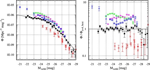
Luminosity functions of quasars at 2 < z < 5. Left: Binned luminosity function. Right: Number ratio of the binned luminosity function at each redshift to the best-fitting model at z ∼ 4. Black filled squares and circles represent the z ∼ 4 quasar luminosity function from the HSC and SDSS DR7 samples, respectively. The solid line indicates the best-fitting double power-law model for the z ∼ 4 luminosity function. Quasar luminosity functions at z ∼ 5 (red crosses: McGreer et al. 2013; asterisks: Yang et al. 2016), z ∼ 3.2 from SDSS/BOSS (Blue open squares: Ross et al. 2013) and COSMOS (blue open triangles: Masters et al. 2012), z ∼ 2.7 (pink open pentagons: Ross et al. 2013), and z ∼ 2.3 (green open circles: Ross et al. 2013) are shown. Binned luminosity functions with Mi(z = 2) are converted to M1450 with M1450 = Mi(z = 2) + 1.486 (Richards et al. 2006). Constant ratios in a redshift range indicate that the luminosity function has the same shape to that of the best-fitting luminosity function at z ∼ 4 except for the normalization. Such evolution corresponds to the pure number evolution. (Color online)
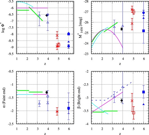
Best-fitting quasar luminosity function parameters (filled diamonds) are compared with those in literature. Green solid lines: Best-fitting PLE and LEDE luminosity function parameters from Ross et al. (2013) below and above z ∼ 2.2, respectively. Cyan solid lines: best-fitting LEDE luminosity function parameters from Croom et al. (2009). Pink solid line: β varying luminosity evolution fit from Bongiorno et al. (2007). Blue dashed line: variable power-law model for bright-end luminosity function from Richards et al. (2006). Blue open triangles: double power-law fit to z ∼ 3.2 and z ∼ 4 luminosity functions from Masters et al. (2012). Blue open circles: double power-law fit to z ∼ 4 luminosity function from Niida et al. (2016). Red cross and asterisk: fit to z ∼ 5 luminosity function from McGreer et al. (2013) with fixed α and β, respectively. Red open square: z ∼ 5 luminosity function from Yang et al. (2016). Blue filled triangles: bright-end z ∼ 6 luminosity function from Willott et al. (2009) with fixed α = −1.5 (large) and α = −1.8 (small). Blue filled circle: z ∼ 6 luminosity function from case 1 of Kashikawa et al. (2015). Blue filled square with thin error bar: z ∼ 6 luminosity function from Jiang et al. (2016). (Color online)
As shown in the bottom right-hand panel of figure 23, the slopes of the bright-end of the luminosity functions are distributed around β = −3 above z = 3, except for the Luminosity Evolution and Density Evolution model in Ross et al. (2013) and Yang et al. (2016) which has steeper bright-end slopes. The value in Ross et al. (2013) is closer to those observed at z < 2 (e.g., Croom et al. 2009) and could be affected by quasars in the redshift range around z = 2. If we compare their binned luminosity functions at z ∼ 2.3 and z ∼ 2.7 with that at z ∼ 4, the slopes above the knee seem to be similar to each other except for the most luminous bins. The bright-end slope above z = 3 being systematically flatter than that at z < 2 is consistent with the trend reported in Richards et al. (2006), Bongiorno et al. (2007), and Richards et al. (2009). The constant bright-end slope above z = 3 would suggest that we do not need a luminosity-dependent evolution model above the knee to explain the increase of the number density at a fixed luminosity (Steffen et al. 2006).
The bottom left-hand panel of figure 23 shows a different trend in the evolution of the faint-end. The luminosity functions at z ∼ 2.3 and 2.7 have a similar shape to the z ∼ 4 luminosity function, and the best-fitting faint-end slope at z = 2.2–3.5 is |$\alpha _{z\,=\,2.2\!-\!3.5}=-1.29^{+0.15}_{-0.03}$| (Ross et al. 2013), which is consistent with the best-fitting value at z ∼ 4 within the 1σ uncertainty. Flat faint-end slope is also supported by Bongiorno et al. (2007), Fontanot et al. (2007), and Niida et al. (2016). On the other hand, the best-fitting model at z ∼ 3.2 has αz = 3.2 = −1.73 ± 0.11 (Masters et al. 2012), which is much steeper than that at z ∼ 4. Such a difference can be seen in the shape of the luminosity functions; the binned z ∼ 3.2 luminosity function does not show a clear knee. Recent measurements of the faint-end slopes at z ∼ 5 (McGreer et al. 2013) and at z ∼ 6 (Kashikawa et al. 2015) are steeper than that at z ∼ 4. However, the current quasar luminosity function at z ∼ 5.0 could not be deep enough to clearly detect the knee of the luminosity function, although the best-fitting value for the faint-end would imply a steeper slope, |$\alpha _{z\,=\,5}=-2.03^{+0.15}_{-0.14}$| (McGreer et al. 2013). Furthermore, the constraint on the faint-end of the quasar luminosity function at z ∼ 6.0 is based on a few quasars (Kashikawa et al. 2015).
In the right-hand panel of figure 22, luminosity functions at z ∼ 2.3, 2.7, and 5 show almost constant ratios in the covered luminosity range, which imply pure density evolution of the quasar luminosity function and no strong evolution in the break luminosity. Such a trend is consistent with the evolutionary trend seen in the X-ray luminosity function at z > 3 (Vito et al. 2014). The constant ratios in the redshift range from z = 2.3 to 5 do not support the higher break luminosities and steeper faint-end slopes with higher redshifts implied above z = 5 (McGreer et al. 2013; Kashikawa et al. 2015).
On the other hand, the ratio of the binned luminosity function at z ∼ 3.2 to that at z ∼ 4 shows a systematic deviation from a constant value; the shape of the luminosity function at z ∼ 3.2 shows a different evolutionary trend than the pure density evolution. In order to conclude the discussion on the evolutionary trend, it is necessary to evaluate the effect of different selection functions at different redshifts in different surveys, and we will leave such further discussions to a later paper.
5.3 Comparison with the X-ray AGN luminosity function
Comparing the luminosity function of the optically selected quasars with that of X-ray-selected AGNs in the same redshift range, we can infer the fraction of blue stellar quasars among the X-ray AGN population, which includes heavily-obscured AGNs. Recent analysis of samples of X-ray selected AGNs indicates that the fraction of heavily-obscured AGNs is higher at z > 3 than that in the local universe (Hiroi et al. 2012; Vito et al. 2013, 2014), and it is possible that the optical selections are missing such heavily-obscured AGNs as discussed in subsection 2.6. In this discussion, we assume both of the AGN populations have the same overall SED, but the optical selection can be affected by the dust extinction and host galaxy contamination.
The resulting hard X-ray luminosity function derived from the optical quasar luminosity function is shown in the left-hand panel of figure 24 as a red thin-dashed line. The black thick solid line indicates the hard X-ray luminosity function of Compton-thin AGNs at z = 3.9 based on the best-fitting luminosity-dependent density evolution (LDDE) model by Ueda et al. (2014). The luminosity function of X-ray-selected AGNs shows higher number density in the entire luminosity range than that of the optically selected quasars, and the discrepancy is broadly consistent with recent comparisons (Marchesi et al. 2016b). However, we need to note that the simple one-to-one conversion from UV to X-ray luminosity (Masters et al. 2012; Marchesi et al. 2016b) may not be appropriate for calculating the converted luminosity function. As discussed in Steffen et al. (2006), at a fixed l2500 Å, the l2 keV values show significant scatter around the mean value, and such scatter can broaden the luminosity function towards the bright-end due to the steep slope of the luminosity function. Therefore, we convert the UV luminosity function by assuming that the UV luminosity is the primary parameter of the quasar luminosity and that the X-ray luminosity has a scatter around the above relation. Using the rms scatter of log (l2 keV) measured in each l2500 Å bin (table 5 of Steffen et al. 2006), we derive the rms scatter as a function of log (l2500 Å).
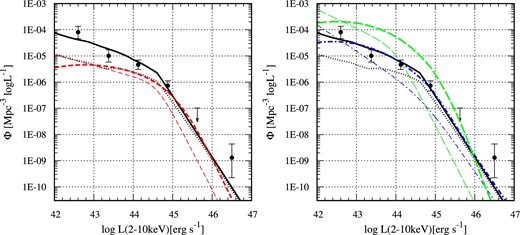
Left: z ∼ 4 quasar 2–10 keV luminosity function predicted from the UV luminosity function of the HSC and SDSS DR7 samples (red dashed lines). Red thick and red thin dashed lines indicate the results with and without the effect of the scatter in the l2500 vs. l2 keV relation. The thick solid line is the best-fitting LDDE model of the 2–10 keV X-ray luminosity function of X-ray selected AGNs at z = 3.9 (Ueda et al. 2014). The thick dotted line indicates the best-fitting X-ray luminosity function for less-absorbed AGNs with log NH(cm−2) <22. Data points for the X-ray luminosity function derived with the ratio of the number of the sample to that of the model prediction are plotted using the filled circles with 1σ error bars. The upper limit without a point indicates the 90% upper limit. Right: 2–10 keV luminosity functions based on the best-fitting UV luminosity functions from Masters et al. (2012) (blue dot–dashed lines) and Giallongo et al. (2015) (green long-dashed lines). Thick and thin lines represent the results with and without the effect of the scatter. Black lines are the same as in the left-hand panel. (Color online)
The resulting hard X-ray luminosity function including the scatter is shown by the red thick-dashed line in the left-hand panel of figure 24. We consider the luminosity range above M1450 < −16.0 mag, which corresponds to log L2 –10 keV(erg s − 1) = 41.91 for the above conversions. Because the number of objects is conserved, the faint-end of the converted luminosity function below log L2 –10 keV(erg s − 1) ∼ 43 shows a decline toward fainter luminosity and it crosses the converted luminosity function at around log L2 –10 keV(erg s − 1) ∼ 42 without the scatter. The resulting X-ray luminosity function shown by the red thick-dashed line is consistent with the best-fitting LDDE model of the X-ray luminosity function at z = 3.9, shown by the black thick solid line, above the knee of the luminosity function at log L2 –10 keV(erg s − 1) ∼ 44.6. The consistency suggests that the current selection of the z ∼ 4 quasars does not miss a significant fraction of quasars that are affected by heavy-obscuration above the knee of the X-ray luminosity function.
Below the knee of the luminosity function, the number density of the converted luminosity function shows a deficiency compared to the hard X-ray luminosity function. The deficiency can be caused by the contribution of obscured and/or less-luminous AGNs which are missed in our selection of z ∼ 4 quasars based on stellar morphology and blue UV color. As shown in subsection 2.6, the z ∼ 4 quasar selection can be missing a significant fraction of AGNs fainter than M1450 ∼ −23.5, which corresponds to log L2 –10 keV(erg s − 1) ∼ 44.1, i.e., 0.5 dex fainter than the knee.
In the left-hand panel of figure 24, the X-ray AGN luminosity function for the less-absorbed AGNs with log NH(cm−2) < 22 is shown with a black thick-dotted line. We assume the column density distribution derived in Ueda et al. (2014). The luminosity function of less-absorbed AGNs shown by the thick dotted line matches well with the converted luminosity function of the optically selected quasars, shown by the red thick-dashed line, down to log L2 –10 keV(erg s − 1) = 43, supporting the theory that the deficiency below the knee is caused by the contribution from the obscured AGNs. Such consistency between the luminosity function of X-ray-selected less-absorbed AGNs and that of optically selected quasars is also shown in Ricci et al. (2017) in a reverse way, i.e., by converting the X-ray luminosity function of Ueda et al. (2014) to the UV luminosity function.
That the luminosity function of the converted X-ray luminosity function with the scatter (red thick-dashed line) is flatter than the best-fitting X-ray luminosity function (thick black solid line) below the knee is consistent with increasing fraction of obscured AGNs with decreasing luminosity. Such a trend follows the luminosity dependence of the fraction observed at z < 3 (e.g., Ueda et al. 2003). Recently, an inverse trend at high redshifts with decreasing fraction of obscured AGNs with decreasing luminosity below the knee has been suggested (Georgakakis et al. 2015), but that trend is not supported in the current result.
The consistency between the luminosity functions of optically selected quasars and X-ray-selected AGNs above the knee could also show a different luminosity dependence of the obscured fraction at z > 3 from that determined with the X-ray-selected AGNs (Vito et al. 2014). Vito et al. (2014) show that the fraction of obscured AGN with a hydrogen column density, log NH (cm−2), larger than 23, does not strongly depend on luminosity in the luminosity range between log L2 –10 keV(erg s − 1) = 43 and 45 with 0.54 ± 0.05. The upper luminosity corresponds to M1450 = −26.7 mag and the luminosity function does not show significant deficiency of optically selected quasars in the luminosity range. This discrepancy would be explained by the luminosity dependence of the relation between the broad-line AGN fraction and the hydrogen column density measured in X-ray (Ueda et al. 2003); a large hydrogen column density can be observed among luminous blue broad-line quasars (e.g., Akiyama et al. 2000; Merloni et al. 2014).
We need to note that the above conversion depends on the assumed l2500 Å–l2 keV relation. If we apply the relation derived in Young et al. (2010), the converted luminosity functions with their results based on CENSORED and SPECTRA samples show a smaller and larger number density than the X-ray luminosity function above the knee, respectively.
We also apply the same conversion to the best-fitting model of the z ∼ 4 luminosity functions from Masters et al. (2012) and Giallongo et al. (2015), and the resulting luminosity functions are shown with blue dot-dashed and green long-dashed lines, respectively, in the right-hand panel of figure 24. Converted luminosity functions with and without the scatter are shown with thick and thin lines, respectively. The resulting luminosity function based on Masters et al. (2012) broadly overlaps with that of the X-ray luminosity function, and they are apparently consistent with each other. However, it should be noted that the quasar sample of Masters et al. (2012) is selected based on similar criteria to ours, employing blue UV color and stellar morphology. Since we expect a significant contribution from obscured and/or fainter AGNs at least below log L2 –10 keV(erg s − 1) ∼ 43, this would imply an overestimation of their luminosity function at the faint-end. Similarly, if we use the best-fitting luminosity function in Giallongo et al. (2015), the converted luminosity function significantly over-predicts the number density, especially below the knee of the luminosity function.
6 Summary
We construct a statistical sample of 1666 z ∼ 4 quasars based on 339.8 deg2 of g-, r-, i-, z-, and y-band imaging data from the S16A-Wide2 release of the HSC-SSP program. The z ∼ 4 quasar candidates are selected by their stellar morphology and g-band dropout selection criteria. Our selection is optimized for selecting stellar objects with as low contamination from extended galaxies as possible. The selection is effective down to i = 24 mag. Our g-dropout color selection criteria is based on the color distributions of SDSS quasars at z = 3.5–4.0 and Galactic stars, which are one of the most numerous contaminants to the selection.
The number counts of the selected z ∼ 4 quasars show a monotonic increase in the covered magnitude range, i = 20.0–24.0, once we correct for the effect of contamination to the selection. The survey selection efficiency and effective survey area are evaluated with libraries of quasar photometric models and a noise model of the HSC stacked images. We evaluate the contamination by Galactic stars and compact galaxies that meet the g-dropout selection criteria. The results indicate that the contamination rate can be more than 50% in the magnitude range fainter than i > 23.5 mag, and the apparent excess seen in the magnitude range of the raw number counts can be explained with this contamination.
Most of the z ∼ 4 quasar candidates do not have spectroscopic redshift information, and we estimate photometric redshifts using a Bayesian method based on our library of quasar models with templates. The distribution of the resulting photometric redshifts implies the sample covers the redshift range between 3.6 to 4.3 with mean redshift of 3.9. The distribution of the UV absolute magnitudes, M1450, estimated from the broad-band photometry, covers an absolute magnitude range down to M1450 ∼ −22 mag, which is more than 2 mag deeper than the SDSS sample. Thanks to the large sample, we determine the faint-end of the z ∼ 4 quasar luminosity function with unprecedented statistics. In order to extend our luminosity coverage to the bright-end, we include the uniform z ∼ 4 quasar sample from the SDSS DR7, providing a combined coverage of M1450 = −22 to −29 mag.
The luminosity function is well described by a double power-law model with a clear break around M1450 ∼ −25 mag. The bright-end slope, β = −3.11 ± 0.07 is consistent with those derived at z = 2.2–3.5 and at z ∼ 5. The faint-end slope, α = −1.30 ± 0.05, is consistent with that at z = 2.2–3.5 obtained from BOSS, but flatter than that derived at z ∼ 3.2 with deeper coverage from the COSMOS survey. The overall shape of the z ∼ 4 luminosity function does not support the higher break luminosities and steeper faint-end slopes at higher redshifts suggested at z ∼ 5 (McGreer et al. 2013).
We convert the M1450 luminosity function to the hard X-ray 2–10 keV luminosity function using the relation between l2500 Å and l2 keV (Steffen et al. 2006). Once we consider the scatter of the relation, the number density of UV-selected quasars matches well with that of the X-ray selected AGNs above the knee of the luminosity function. Below the knee of the luminosity function, the UV-selected quasars show a deficiency compared to the hard X-ray luminosity function. The deficiency can be explained by obscured AGNs.
Acknowledgements
We would like to thank the referee for his invaluable comments, which improved the manuscript. We thank Dr. Akio K. Inoue for providing us with the updated Monte Carlo model of the IGM absorption.
The Hyper Suprime-Cam (HSC) collaboration includes the astronomical communities of Japan and Taiwan, and Princeton University. The HSC instrumentation and software were developed by the National Astronomical Observatory of Japan (NAOJ), the Kavli Institute for the Physics and Mathematics of the Universe (Kavli IPMU), the University of Tokyo, the High Energy Accelerator Research Organization (KEK), the Academia Sinica Institute for Astronomy and Astrophysics in Taiwan (ASIAA), and Princeton University. Funding was contributed by the FIRST program from Japanese Cabinet Office, the Ministry of Education, Culture, Sports, Science and Technology (MEXT), the Japan Society for the Promotion of Science (JSPS), Japan Science and Technology Agency (JST), the Toray Science Foundation, NAOJ, Kavli IPMU, KEK, ASIAA, and Princeton University.
This paper makes use of software developed for the Large Synoptic Survey Telescope. We thank the LSST Project for making their code available as free software at 〈http://dm.lsst.org〉.
The Pan-STARRS1 Surveys (PS1) have been made possible through contributions of the Institute for Astronomy, the University of Hawaii, the Pan-STARRS Project Office, the Max-Planck Society and its participating institutes, the Max Planck Institute for Astronomy, Heidelberg and the Max Planck Institute for Extraterrestrial Physics, Garching, The Johns Hopkins University, Durham University, the University of Edinburgh, Queen’s University Belfast, the Harvard-Smithsonian Center for Astrophysics, the Las Cumbres Observatory Global Telescope Network Incorporated, the National Central University of Taiwan, the Space Telescope Science Institute, the National Aeronautics and Space Administration under Grant No. NNX08AR22G issued through the Planetary Science Division of the NASA Science Mission Directorate, the National Science Foundation under Grant No. AST-1238877, the University of Maryland, and Eotvos Lorand University (ELTE) and the Los Alamos National Laboratory.
This paper is based in part on data collected at the Subaru Telescope and retrieved from the HSC data archive system, which is operated by Subaru Telescope and Astronomy Data Center, National Astronomical Observatory of Japan.
Funding for the Sloan Digital Sky Survey IV has been provided by the Alfred P. Sloan Foundation, the U.S. Department of Energy Office of Science, and the Participating Institutions. SDSS-IV acknowledges support and resources from the Center for High-Performance Computing at the University of Utah. The SDSS web site is 〈www.sdss.org〉.
SDSS-IV is managed by the Astrophysical Research Consortium for the Participating Institutions of the SDSS Collaboration including the Brazilian Participation Group, the Carnegie Institution for Science, Carnegie Mellon University, the Chilean Participation Group, the French Participation Group, Harvard-Smithsonian Center for Astrophysics, Instituto de Astrofísica de Canarias, The Johns Hopkins University, Kavli Institute for the Physics and Mathematics of the Universe (IPMU) / University of Tokyo, Lawrence Berkeley National Laboratory, Leibniz Institut für Astrophysik Potsdam (AIP), Max-Planck-Institut für Astronomie (MPIA Heidelberg), Max-Planck-Institut für Astrophysik (MPA Garching), Max-Planck-Institut für Extraterrestrische Physik (MPE), National Astronomical Observatories of China, New Mexico State University, New York University, University of Notre Dame, Observatário Nacional / MCTI, The Ohio State University, Pennsylvania State University, Shanghai Astronomical Observatory, United Kingdom Participation Group, Universidad Nacional Autónoma de México, University of Arizona, University of Colorado Boulder, University of Oxford, University of Portsmouth, University of Utah, University of Virginia, University of Washington, University of Wisconsin, Vanderbilt University, and Yale University.
Footnotes
References
