


Abstract
We examine the clustering of quasars over a wide luminosity range, by utilizing 901 quasars at |$\overline{z}_{\rm phot}\sim 3.8$| with −24.73 < M1450 < −22.23 photometrically selected from the Hyper Suprime-Cam Subaru Strategic Program (HSC-SSP) S16A Wide2 date release and 342 more luminous quasars at 3.4 < zspec < 4.6 with −28.0 < M1450 < −23.95 from the Sloan Digital Sky Survey that fall in the HSC survey fields. We measure the bias factors of two quasar samples by evaluating the cross-correlation functions (CCFs) between the quasar samples and 25790 bright z ∼ 4 Lyman break galaxies in M1450 < −21.25 photometrically selected from the HSC dataset. Over an angular scale of 10|${^{\prime\prime}_{.}}$|0 to 1000|${^{\prime\prime}_{.}}$|0, the bias factors are |$5.93^{+1.34}_{-1.43}$| and |$2.73^{+2.44}_{-2.55}$| for the low- and high-luminosity quasars, respectively, indicating no significant luminosity dependence of quasar clustering at z ∼ 4. It is noted that the bias factor of the luminous quasars estimated by the CCF is smaller than that estimated by the auto-correlation function over a similar redshift range, especially on scales below 40|${^{\prime\prime}_{.}}$|0. Moreover, the bias factor of the less-luminous quasars implies the minimal mass of their host dark matter halos is 0.3–2 × 10¹² h−1 M⊙, corresponding to a quasar duty cycle of 0.001–0.06.
1 Introduction
It is our current understanding that every massive galaxy is likely to have a supermassive black hole (SMBH) at its center (Kormendy & Richstone 1995). Active galactic nuclei (AGNs) are thought to be associated with the growth phase of the BHs through mass accretion. Being the most luminous of the AGN populations, quasars may be the progenitors of the most massive SMBHs in the local universe. Observations over the last decade or so are establishing a series of scaling relations between SMBH mass and properties of their host galaxies (for review see Kormendy & Ho 2013). A similar scaling relation, involving the mass of the SMBH, is reported even with the host dark matter halo (DMH) mass (Ferrarese 2002). As a result, SMBHs are thought to play an important role in galaxy formation and evolution. However, the physical mechanism behind the scaling relations is still unclear.
Clustering analysis of AGNs is commonly used to investigate SMBH growth and galaxy evolution in DMHs. Density peaks in the underlying dark matter distribution are thought to evolve into DMHs (e.g., Press & Schechter 1974), in which the entire structure is gravitationally bound with a density 300 times higher than the mean density of the universe. More massive DMHs are formed from rarer density peaks in the early universe, and are more strongly clustered (e.g., Sheth & Torman 1999; Sheth et al. 2001). If focusing on the large-scale clustering, i.e., two-halo term, the mass of quasar host halos can be inferred by estimating the clustering strength of quasars in relative to that of the underlying dark matter, i.e., the bias factor. How the bias factor of quasars depends on redshift and luminosity provides further information on the relation between SMBHs and galaxies within their shared DMH.
Many studies, based on the two-point correlation function (2PCF) of quasars, have been conducted by utilizing large databases of quasars, such as the 2dF Quasar Redshift Survey (e.g., Croom et al. 2005) and the Sloan Digital Sky Survey (SDSS; e.g, Myers et al. 2007; Shen et al. 2009; White et al. 2012). The redshift evolution of the auto-correlation function (ACF) indicates that quasars are more strongly biased at higher redshifts. For example, luminous SDSS quasars with −28.2 < M1450 < −25.8 at z ∼ 4 show strong clustering with a bias factor of 12.96 ± 2.09, which corresponds to a host DMH mass of ∼1013 h−1 M⊙ (Shen et al. 2009). It is suggested that such high luminosity quasar activity needs to be preferentially associated with the most massive DMHs in the early universe (White et al. 2008). If we consider the low number density of such massive DMHs at z = 4, the fraction of halos with luminous quasar activity is estimated to be 0.03–0.6 (Shen et al. 2007) or up to 0.1–1 (White et al. 2008).
The clustering strength of quasars can be also measured from the cross-correlation function (CCF) between quasars and galaxies (e.g., Adelberger & Steidel 2005; Francke et al. 2007; Font-Ribera et al. 2013). When the size of a quasar sample is limited, the clustering strength of the quasars can be constrained with higher accuracy by using the CCF rather than the ACF since galaxies are usually more numerous than quasars. Enhanced clustering and overdensities of galaxies around luminous quasars are expected from the strong auto-correlation of the SDSS quasars at z ∼ 4. However, observational searches for such overdensities around quasars at high redshifts have not been conclusive. While some luminous z > 3 quasars are found to be in an over-dense region (e.g., Zheng et al. 2006; Kashikawa et al. 2007; Utsumi et al. 2010; Capak et al. 2011; Adams et al. 2015; Garcia-Vergara et al. 2017), a significant fraction of them do not show any surrounding overdensity compared to the field galaxies, and it is suggested that the large-scale (∼10 comoving Mpc) environment around the luminous z > 3 quasars is similar to the Lyman break galaxies (LBGs), i.e., typical star-forming galaxies, in the same redshift range (e.g., Kim et al. 2009; Bañados et al. 2013; Husband et al. 2013; Uchiyama et al. 2018).
To investigate the quasar environment at z ∼ 4, the clustering of quasars with lower luminosity at MUV ≳ −25, i.e., typical quasars, which are more abundant than luminous SDSS quasars, is crucial that it can constrain the growth of SMBHs inside galaxies in the early universe (Hopkins et al. 2007). At low redshifts (z ≲ 3), clustering of quasars is found to have no or weak luminosity dependence (e.g., Francke et al. 2007; Shen et al. 2009; Krumpe et al. 2010; Shirasaki et al. 2011). Above z > 3, Ikeda et al. (2015) examined the CCF of 25 less-luminous quasars in the COSMOS field. However, since the sample size is small, the clustering strength of the less-luminous quasars has still not been well constrained, and their correlation with galaxies remains unclear.
The wide and deep multi-band imaging dataset of the Subaru Hyper Suprime-Cam Strategic Survey Program (HSC-SSP: Aihara et al. 2018a) provides us with a unique opportunity to examine the clustering of galaxies around high-redshift quasars in a wide luminosity range. Based on an early data release of the survey (S16A: Aihara et al. 2018b), a large sample of less-luminous z ∼ 4 quasars (MUV < −21.5) is constructed for the first time (Akiyama et al. 2018). They cover the luminosity range around the knee of the quasar luminosity function, i.e., they are typical quasars in the redshift range. Additionally, more than 300 SDSS luminous quasars at z ∼ 4 fall within the HSC survey area thanks to a wide field of 339.8 deg2. Likewise, the five bands of HSC imaging are deep enough to construct a sample of galaxies in the same redshift range through the Lyman-break method (Steidel et al. 1996).
Here, we examine the clustering of galaxies around z ∼ 4 quasars over a wide luminosity range of −28.0 < M1450 < −22.2 by utilizing the HSC-SSP dataset. By comparing the clustering of the luminous and less-luminous quasars, we can further evaluate the luminosity dependence of the quasar clustering. The outline of this paper is as follows. Section 2 describes the samples of z ∼ 4 quasars and LBGs. Section 3 reports the results of the clustering analysis, and we discuss the implication of the observed clustering strength in section 4. Throughout this paper, we adopt a ΛCDM model with cosmological parameters of H0 = 70 km s−1 Mpc−1 (h = 0.7), Ωm = 0.3, ΩΛ = 0.7, and σ8 = 0.84. All magnitudes are described in the AB magnitude system.
2 Data
2.1 HSC-SSP Wide layer dataset
We select the candidates of z ∼ 4 quasars and LBGs from the Wide layer catalog of the HSC-SSP (Aihara et al. 2018a). HSC is a wide-field mosaic CCD camera, which is attached to the prime-focus of the Subaru telescope (Miyazaki et al. 2012, 2018). It covers a field of view (FoV) of 1.°5 diameter with 116 full-depletion CCDs, which have a high sensitivity up to 1 μm. The Wide layer of the survey is designed to cover 1400 deg2 in the g, r, i, z, and y bands with 5σ detection limits of 26.8, 26.4, 26.4, 25.5, and 24.7, respectively, in the five-year survey (Aihara et al. 2018a). In this analysis, we use the S16A Wide2 internal data release (Aihara et al. 2018b), which covers 339.8 deg2 in the five bands, including edge regions where the depth is shallower than the final depth. The data are reduced with hscPipe-4.0.2 (Bosch et al. 2018).
The astrometry of the HSC imaging is calibrated by the Pan-STARRS 1 Processing Version 2 (PS1 PV2) data (Magnier et al. 2013), which covers all HSC survey regions to a reasonable depth with a similar set of bandpasses (Aihara et al. 2018b). It is found that the rms of stellar object offsets between the HSC and PS1 positions is ∼40 mas. Extended galaxies have additional offsets with rms values of ∼30 mas in relative to the stellar objects (Aihara et al. 2018b).
We use PSF magnitudes for stellar objects and CModel magnitudes for extended objects. PSF magnitudes are determined by fitting a model PSF, while CModel magnitudes are determined by fitting a linear combination of exponential and de Vaucouleurs profiles convolved with the model PSF at the position of each object. We correct for galactic extinction in all five bands based on the dust extinction maps by Schlegel, Finkbeiner, and Davis (1998). Only objects that have magnitude errors in the r and i bands smaller than 0.1 are considered.
2.2 Samples of z ∼ 4 quasars
|${\rm i\_hsm\_moments\_11} {\rm (22)}$| is the second-order adaptive moment of an object in the x (y) direction determined with the algorithm described in Hirata and Seljak (2003) and |${\rm i\_hsm\_psfmoments\_11} {\rm (22)}$| is that of the model PSF at the object position. The i-band adaptive moments are adopted since the i-band images are selectively taken under good seeing conditions (Aihara et al. 2018b). Objects that have the adaptive moment with “nan” are removed. Since stellar objects should have an adaptive moment that is consistent with that of the model PSF, we set the above stellar/extended classification criteria. The selection completeness and the contamination are examined by Akiyama et al. (2018). At i < 23.5, the completeness is above 80% and the contamination from extended objects is lower than 10%. At fainter magnitudes (i > 23.5), the completeness rapidly declines to less than 60% and the contamination sharply increases to greater than 10% (see the middle panel of figure 1 in Akiyama et al. 2018). To avoid severe contamination by extended objects, we limit the faint end of the quasar sample to i = 23.5.
i-band magnitude distributions of the samples. Left: Red and black histograms show the distributions of the z ∼ 4 quasar candidates from the HSC-SSP and SDSS, respectively. Right: The blue histogram represents the distribution of the z ∼ 4 LBGs from the HSC-SSP. (Color online)
We apply the Lyman-break selection to identify quasars at z ∼ 4. The selection utilizes the spectral property that the continuum blue-ward of the Lyα line (λrest = 1216 Å) is strongly attenuated by absorption due to the intergalactic medium (IGM). The Lyα line of an object at z = 4.0 is redshifted to 6075 Å in the observed frame, which is in the middle of the r-band, as a result the object has a red g − r color. We apply the same color selection criteria as described in Akiyama et al. (2018). In total, 1023 z ∼ 4 quasar candidates in the magnitude range 20.0 < i < 23.5 are selected. We limit the bright end of the sample considering the effects of saturation and non-linearity. Even though we include edge regions with a shallow depth for the sample selection, we do not find a significant difference of the number densities in the edge and central regions. Therefore, we conclude that larger photometric uncertainties or a higher number density of junk objects in the shallower regions do not result in higher contamination for quasars in the region. The i-band magnitude distribution of the sample is shown with the red histogram in the left-hand panel of figure 1.
The completeness of the color selection is examined with the 3.5 < zspec < 4.5 SDSS quasars with i > 20.0 within the HSC coverage (Akiyama et al. 2018). Among 92 SDSS quasars with clean HSC photometry, 61 of them pass the color selection, resulting in the completeness of 66%. Since the sample is photometrically selected, it can be contaminated by galactic stars and compact galaxies that meet the color selection criteria. The contamination rate is further evaluated by using mock samples of galactic stars and galaxies; the contamination rate is less than 10% at i < 23.0, and increases to more than 40% at i ∼ 23.5. It causes an excess of HSC quasars in faint magnitude bins (23.2 < i < 23.5) as shown in the left-hand panel of figure 1. Since the contamination rate sharply increases at i > 23.5, we limit the sample at this magnitude. For the bright end, as the luminous SDSS quasar sample primarily includes quasars brighter than i = 21.0, we consider the HSC quasar sample fainter than i = 21.0 to constitute the less-luminous quasar sample. Finally, 901 quasars from the HSC are selected in the magnitude range of 21.0 < i < 23.5. Here, we convert the i-band apparent magnitude to the UV absolute magnitude at 1450 Å using the average quasar SED template provided by Siana et al. (2008) at z ∼ 4, which results in a magnitude range of −24.73 < M1450 < −22.23. In Akiyama et al. (2018), a best-fitting analytic formula of the contamination rate as a function of the i-band magnitude is provided. If we apply it to the less-luminous quasar sample, it is expected that 90 out of 901 candidates are contaminating objects, i.e., contamination rate of the z ∼ 4 less-luminous quasar sample is 10.0%.
The redshift distribution of the z ∼ 4 less-luminous quasar candidates is shown in figure 2 with the red histogram. For 32 candidates with spectroscopic redshift information, we adopt their spectroscopic redshifts, otherwise the redshifts are estimated with a Bayesian photometric redshift estimator using a library of mock quasar templates (Akiyama et al. 2018). Most of the quasars are in the redshift range between 3.4 and 4.6. Average and standard deviation of the redshift distribution are 3.8 and 0.2, respectively.
Redshift distributions of the samples. The red histogram indicates the redshift distribution of the less-luminous quasar sample determined either spectroscopically or photometrically (Akiyama et al. 2018). The black dashed histogram shows the spectroscopic redshift distribution of the luminous quasar sample. The blue histogram represents the expected redshift distribution of the LBG sample evaluated with the mock LBGs (see text in subsection 2.4). All histograms are normalized so that |$\int _{0}^{\infty }N(z)dz=1$|. (Color online)
In order to examine the luminosity dependence of the quasar clustering, a sample of luminous z ∼ 4 quasars is constructed based on the 12th spectroscopic data release of the Sloan Digital Sky Survey (SDSS) (Alam et al. 2015). We select quasars with criteria on object type (“QSO”), reliability of the spectroscopic redshift (“z_waring” flag = 0), and estimated redshift error (smaller than 0.1). Only quasars within the coverage of the HSC S16A Wide2 data release are considered. We limit the redshift range between 3.4 and 4.6 following the redshift distribution of the HSC z ∼ 4 LBG sample (which will be discussed in subsection 2.4). In the coverage of the HSC S16A Wide2 data release, there are 342 quasars that meet the selection criteria. Their redshift distribution is shown by black dashed histogram in figure 2. Average and standard deviation of the redshift distribution are 3.77 and 0.26, respectively. Although the redshift distribution of the SDSS sample shows excess around z ∼ 3.5 compared to the HSC sample, the average and standard deviations are close to each other.
The i-band magnitude distribution of the SDSS quasars is plotted by the black histogram in the left-hand panel of figure 1. To determine their i-band magnitude in the HSC photometric system, we match the sample to HSC clean objects using a search radius of 1|${^{\prime\prime}_{.}}$|0. Out of the 342 SDSS quasars, 296 have a corresponding object among the clean objects, while the others are saturated in the HSC imaging data. For the remaining 46 quasars, we convert their r- and i-band magnitudes in the SDSS system to the i-band magnitude in the HSC system following the equations in subsection 3.3 in Akiyama et al. (2018). As can be seen from the distributions, the SDSS quasar sample covers a magnitude range about 2 mag brighter than the HSC quasar sample. Their corresponding UV absolute magnitudes at 1450 Å are in the range of −28.0 to −23.95 evaluated by the same method with the less-luminous quasar sample.
2.3 Sample of z ∼ 4 LBGs from the HSC dataset
We select candidates of z ∼ 4 LBGs from the S16A Wide2 dataset in the similar way as we select the z ∼ 4 quasar candidates. Unlike the process for quasars, we select candidates from the extended clean objects instead of the stellar objects, i.e., we pick out the clean objects that do not meet either of the equations (6) or (7) as extended objects. As shown in figure 9 of Akiyama et al. (2018), extended galaxies at z > 3 are distinguishable from stellar quasars with these criteria, as a result of the good image quality of the i-band HSC Wide layer images, which has a median seeing size of 0|${^{\prime\prime}_{.}}$|61 (Aihara et al. 2018b). While the stellar/extended classification is ineffective at i > 23.5, the contamination of stellar objects to the LBG sample is negligible, because the extended objects outnumber the stellar objects by ∼30 times at 23.5 < i < 25.0.
We determine the color selection criteria of z ∼ 4 LBGs based on color distributions of a library of model LBG spectral energy distributions (SEDs), because the sample of z ∼ 4 LBGs with a spectroscopic redshift at the depth of the HSC Wide layer is limited. The model SEDs are constructed with the stellar population synthesis model by Bruzual and Charlot (2003). We assume a Salpeter initial mass function (Salpeter 1955) and the Padova evolutionary track for stars (Fagotto et al. 1994a, 1994b, 1994c) of solar metallicity. Following a typical star-formation history of z ∼ 4 LBGs derived based on an optical–NIR SED analysis (e.g., Shapley et al. 2001; Nonino et al. 2009; Yabe et al. 2009), we adopt an exponentially declining star-formation history with ψ(t) = τ−1exp(−t/τ), where τ = 50 Myr and t = 300 Myr. In addition to the stellar continuum component, we also consider the Lyα emission line at 1216 Å with a equivalent width (EWLyα) randomly distributed within the range between 0 and 30 Å, which is determined to follow the Lyα EW distribution of luminous LBGs in the UV absolute magnitude range of −23.0–−21.5 (Ando et al. 2006). We apply extinction as a screen dust with the dust extinction curve of Calzetti et al. (2000). We assume that E(B − V) has a Gaussian distribution with a mean of 0.14 and 1σ of 0.07 following that observed for z ∼ 3 UV-selected galaxies (Reddy et al. 2008). In order to reproduce the observed scatter of the g − r color of galaxies at z ∼ 3 (see figure 3), the scatter of the color excess is doubled to σ = 0.14. In total, 3000 SED templates are constructed. Each template is redshifted to z = 2.5–5.0 with an interval of 0.1. Attenuation by the intergalactic medium is applied to the redshifted templates. We follow the updated number density of the Lyα absorption systems in Inoue et al. (2014), and consider scatter in the number density of the systems along different line of sights with the Monte Carlo method used in Inoue and Iwata (2008). In figure 3, we compare the distributions of the g − r and r − z colors of the templates with those of spectroscopically confirmed LBGs at i < 24.5 in the HSC-SSP catalogs of the Ultra-Deep layer. Since spectroscopically-identified LBGs selected from narrow-band colors are biased towards LBGs with large Lyα EW, we remove them in the spectroscopically-identified sample. The color distribution of the mock LBGs as a function of redshift reproduces that of the galaxies with spectroscopic redshifts around 3. At z > 3.5, real galaxies follow the color evolution trend of the mock LBGs with slightly bluer g − r and r − z colors. Since the discrepancy is within the scatter and size of sample is limited, we adopt the current mock LBG library in this work.
g − r (left) and r − z (right) colors versus redshift of the mock LBGs. The red line and the error bars are the average and 1σ scatter of the colors of the mock LBGs. Blue points represent spectroscopically confirmed galaxies within the HSC S16A Ultra-Deep layer. (Color online)
Color selection of z ∼ 4 LBGs. Blue crosses and black triangles are galaxies at 0.2 < z < 0.8 and 0.8 < z < 3.5, respectively. Only 5.0% of them are plotted, for clarity. Red stars are galaxies at 3.5 < z < 4.5. Purple inverted triangle is galaxy at z > 4.5. Green dots are colors of stars derived in the spectro-photometric catalog by Gunn and Stryker (1983). The solid black line is the track of the model LBG. Black squares and error bars denote the average and 1σ color scatter of the mock LBGs along the track at z = 2.5, 3.0, 3.5, 4.0, and 4.4. Pink shaded area implies the 1σ r − z scatter of the mock LBGs. Blue dashed lines represent our selection criteria. (Color online)
2.4 Redshift distribution and contamination rate of the z ∼ 4 LBG sample
The redshift distribution of the LBG sample is evaluated by applying the same selection criteria to a sample of mock LBGs, which are constructed in the redshift range between 3.0 and 5.0 with a 0.1 redshift bin. At each redshift bin, we randomly select LBG templates from our library of SEDs and normalize them to have 22.0 < i < 24.5 following the LBG UV luminosity function at z ∼ 3.8 (van der Burg et al. 2010). We convert the apparent i-band magnitude to the absolute UV magnitude based on the selected templates. It should be noted that an object with a fixed apparent magnitude has a higher luminosity and a smaller number density in the luminosity function at higher redshifts. We also consider the difference in comoving volume at each redshift bin.
For each redshift bin, we then place the mock LBGs at random positions in the HSC Wide layer images with a density of 2000 galaxies per deg2, and apply the same masking process as for the real objects. We calculate the expected photometric error at each position using the relation between the flux uncertainty and the value of image variance. This relation is determined empirically with the flux uncertainty of real objects as a function of the PSF and object size. The variance is measured within 1″ × 1″ at each point. The size of the model PSF at the position is evaluated with the model PSF of the nearest real object in the database. In order to reproduce the photometric error associated with the real LBGs, we use the relation for a size of 1|${^{\prime\prime}_{.}}$|5. After calculating the photometric error with this method, we add a random photometric error assuming the Gaussian distribution. Finally, we apply the color selection criteria and remove mock LBGs with magnitude errors larger than 0.1 in either of the i or r bands. The ratio of the recovered mock LBGs to the full random mock LBGs is evaluated as the selection completeness at each redshift bin. We find that the selection completeness is ∼10.0%–30.0% in the redshift range between 3.5 and 4.2, but smaller than 5% at other redshifts. These low rates are due to the fact that we set stringent constraints so that we can prevent the severe contamination from low-redshift galaxies. Based on a selection completeness of 20.0% at 3.5 < z < 4.2, we calculate an expected number of 35988 LBGs with 22 < i < 24.5 in the HSC-SSP S16A Wide layer from the LBG UV luminosity function at z ∼ 3.8 (van der Burg et al. 2010), which is larger than the actual LBG sample size (25790) in this work since we consider the edge regions that have a shallow depth. The effect of the shallow depth is considered in the construction of the random objects (subsection 2.5).
The redshift distribution is measured by multiplying the completeness ratio with the number of mock LBGs at each redshift, which is shown in figure 2 by the blue histogram. The average and 1σ of the distribution is 3.71 and 0.30, respectively. The redshift distribution of the LBGs is similar to that of the luminous quasar sample, but slightly extended toward lower redshifts than the less-luminous quasar sample. It is likely that the extension is due to the higher number density of LBGs in 22.0 < i < 24.5 at 3.3 < z < 3.5.
The LBG sample can be contaminated by low-redshift red galaxies which have similar photometric properties to the z ∼ 4 LBGs. We evaluate the contamination rate of the LBG selection using the HSC photometry in the COSMOS region and the COSMOS i-band selected photometric redshift catalogue, which is constructed by a χ2 template-fitting method with 30 broad, intermediate, and narrow bands from UV to mid-IR in the 2 deg2 COSMOS field (Ilbert et al. 2009). In the HSC-SSP S15B internal database, three stacked images in the COSMOS region, simulating good, median, and bad seeing conditions, are provided. Since the i-band images of the Wide layer are selectively taken under good or median seeing conditions (Aihara et al. 2018b), we match the catalogs from the median stacked image, which has a FWHM of 0|${^{\prime\prime}_{.}}$|70, with galaxies in the photometric redshift catalog within an angular separation of 1|${^{\prime\prime}_{.}}$|0. As examined by Ilbert et al. (2009), the photometric redshift uncertainty of galaxies with COSMOS i΄-band magnitudes brighter than 24.0 is estimated to be smaller than 0.02 at z < 1.25. For galaxies within the same luminosity range at higher redshifts, 1.25 < z < 3, the uncertainty is significantly higher but roughly below 0.1. Thus we only include objects with photometric redshift uncertainties less than 0.02 and 0.1 at z < 1.25 and at z > 1.25, respectively, in the matched catalog. We apply the color selection criteria (8)–(12) to the matched catalog. Among 700 matched galaxies with 3.5 < zphot < 4.5, 117 galaxies pass the selection criteria, resulting in the completeness of 17%, which is consistent with that examined by the mock LBGs. Meanwhile, we investigate the contamination by the ratio of galaxies at z < 3 or z > 5 among those passing the selection criteria at each magnitude bin of 0.1. It is found that the contamination rate is 10% to 30% in the magnitude range of i = 23.5–24.5, and sharply increases to >50% at i = 25.0. In total, all contaminating sources are classified to be at z < 3, while 95% of them are at z < 1. We multiply the contamination rate as a function of the i-band magnitude with the number counts of the LBG candidates at each 0.1 bin to estimate the total number of contaminating sources in the sample. Among 25790 LBG candidates, 5886 are expected to be contaminating objects at z < 3, i.e., the contamination rate is 22.8%.
Furthermore, we also check the photometric redshift of the LBG candidates determined with the five-band HSC Wide layer photometry via the MIZUKI photometric redshift code, which uses the Bayesian photometric redshift estimation (Tanaka et al. 2018). Among the 25790 z ∼ 4 LBG candidates, 25749 of them have photometric redshifts with the MIZUKI code, and 4091 of them have photometric redshifts lower than z = 3.0. The contamination rate is evaluated to be 15.9%, which is similar to the one evaluated in the COSMOS region. Since the COSMOS photometric redshift catalog is based on the 30-band photometry covering a wider wavelength range, we consider the contamination rate evaluated in the COSMOS region in the later clustering analysis.
2.5 Constructing random objects for the clustering analysis
The clustering strength is evaluated by comparing the number of pairs of real objects and that of mock objects distributed randomly in the survey area. Therefore it is necessary to construct a sample of mock objects that are distributed randomly within the survey area and are selected with the same selection function as the real sample. From z = 3 to 5, we construct 3000 mock LBG SEDs, which are normalized to have i = 24.5, at each 0.1 redshift bin. Then we place the mock LBGs randomly over the survey region with a surface number density of 2000 LBGs per deg2, with errors as described in subsection 2.4. After applying the same color selection and magnitude error criteria as for the real objects, we create a sample of 150756 random LBGs, which reproduces the global distribution of the real LBGs including the edge of the survey region where the depth is shallower. Therefore, the clustering analysis on large scales is not affected by the discrepancy of the sky coverage between the quasars and LBGs.
Furthermore, since the detection completeness can be affected by non-uniform seeing within the Wide layer dataset especially at i = 24.5, it is important to reproduce the seeing dependence of the LBG detection completeness in the construction of the random LBGs. Over the entire clean area, 11.2% and 12.1% patches are taken under seeing smaller than 0|${^{\prime\prime}_{.}}$|5 and greater than 0|${^{\prime\prime}_{.}}$|7, respectively. For the LBG sample at i < 24.5, there are 15.8% and 7.7% of them taken under seeing smaller than 0|${^{\prime\prime}_{.}}$|5 and greater than 0|${^{\prime\prime}_{.}}$|7, respectively, suggesting a higher (lower) detection completeness with better (worse) seeing. We plot the cumulative probability functions (CPFs) of the seeing for LBGs, random LBGs, and the entire clean region in figure 5. It can be seen that the random LBGs reproduce the seeing dependence of the detection completeness.
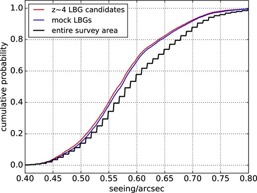
Cumulative probability functions of the i-band seeing at the position of the selected z ∼ 4 LBG candidates (red line), random LBGs (blue line) and entire clean area (black line). (Color online)
3 Clustering analysis
3.1 Cross-correlation functions of the less-luminous and luminous quasars at z ∼ 4
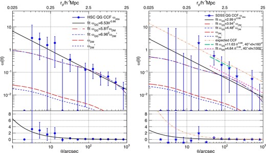
Left-hand panel: Blue dots are the observed mean CCF ωobs of the less-luminous quasars and the LBGs at z ∼ 4 obtained from the Jackknife resampling. The black solid line is the best-fitting power-law model using ML fitting on the scale of 10|${^{\prime\prime}_{.}}$|0 to1000|${^{\prime\prime}_{.}}$|0. The red dash–dotted line is the best-fitting dark matter model ωDM (red long-dashed line) adopting ML fitting in the same scale based on the HALOFIT power spectrum (Smith et al. 2003), while the blue dash–dotted line is the best-fitting dark matter model |$\omega _{\rm DM}^{\prime }$| (blue short-dashed line) after considering the contaminations of the less-luminous quasars and the LBGs. Right-hand panel: Blue stars are the observed mean CCF ωobs of the luminous quasars and the LBGs at z ∼ 4 got from the Jackknife resampling. Red and blue lines have the same meaning as in the the left-hand panel but the blue line only considers the contamination of the LBGs. The orange dash–double-dotted line is the expected CCF of the luminous quasars estimated by the luminous quasars ACF in Shen et al. (2009). The green thick long-dashed and pink thick dashed lines are the best-fitting power-law models on the scale of 40|${^{\prime\prime}_{.}}$|0 to 160|${^{\prime\prime}_{.}}$|0 and of 40|${^{\prime\prime}_{.}}$|0 to 1000|${^{\prime\prime}_{.}}$|0, respectively. In both of the panels, symbols just on the horizontal axis with no error bar beyond 10|${^{\prime\prime}_{.}}$|0, those with no error bar within 10|${^{\prime\prime}_{.}}$|0, and those with error bars in the top pad mean negative bins with a small error bar, zero bins without pair count, and negative or zero bins with a large error bar, respectively. Top and bottom panels show the logarithmic and the linear scale of the vertical axis, respectively. The top horizontal axis of the top panel implies the comoving distance at redshift 4. (Color online)
Less-luminous and luminous quasar–LBG CCFs at z ∼ 4.
| θ (″) | (θmin, θmax) | Less-luminous | Luminous | ||||||||
|---|---|---|---|---|---|---|---|---|---|---|---|
| 〈DQDG〉 | 〈DQRG〉 | ω(θ) | |$\overline{\omega _{i}(\theta )}$| | σ(θ) | 〈DQDG〉 | 〈DQRG〉 | ω(θ) | |$\overline{\omega _{i}(\theta )}$| | σ(θ) | ||
| 2.05 | (1.58, 2.51) | 0 | 0 | 0 | 0 | 0 | 0 | 0 | 0 | 0 | |
| 3.25 | (2.51, 3.98) | 2 | 3 | 2.90 | 3.25 | 8.74 | 0 | 1 | −1 | −1 | 9.76 |
| 5.15 | (3.98, 6.31) | 4 | 6 | 2.90 | 2.86 | 2.51 | 3 | 0 | 0 | 0 | 8.53 |
| 8.15 | (6.31, 10.00) | 3 | 7 | 1.51 | 1.58 | 1.91 | 0 | 4 | −1 | −1 | 1.69 |
| 12.92 | (10.00, 15.85) | 5 | 10 | 1.92 | 1.96 | 1.79 | 1 | 9 | −0.35 | −0.33 | 0.86 |
| 20.48 | (15.85, 25.12) | 7 | 47 | −0.13 | −0.11 | 0.47 | 3 | 6 | 1.92 | 1.96 | 2.11 |
| 32.46 | (25.12, 39.81) | 28 | 120 | 0.36 | 0.36 | 0.26 | 1 | 41 | −0.86 | −0.85 | 0.15 |
| 51.45 | (39.81, 63.10) | 52 | 303 | 0.003 | −0.002 | 0.18 | 25 | 96 | 0.52 | 0.53 | 0.32 |
| 81.55 | (63.10, 100.00) | 143 | 739 | 0.13 | 0.13 | 0.13 | 47 | 226 | 0.22 | 0.21 | 0.27 |
| 129.24 | (100.00, 158.49) | 334 | 1710 | 0.14 | 0.14 | 0.09 | 116 | 589 | 0.15 | 0.15 | 0.14 |
| 204.84 | (158.49, 251.19) | 754 | 4144 | 0.06 | 0.06 | 0.04 | 257 | 1407 | 0.07 | 0.07 | 0.08 |
| 324.65 | (251.19, 398.11) | 1887 | 10375 | 0.06 | 0.06 | 0.04 | 585 | 3677 | −0.07 | −0.07 | 0.04 |
| 514.53 | (398.11, 630.96) | 4564 | 25764 | 0.04 | 0.04 | 0.02 | 1669 | 9272 | 0.05 | 0.05 | 0.07 |
| 815.48 | (630.96, 1000.00) | 11065 | 63358 | 0.02 | 0.02 | 0.02 | 3967 | 23241 | −0.002 | −0.005 | 0.03 |
In this study, we focus on the large-scale clustering between two halos, i.e., the two-halo term. Thus the excess within an individual halo (one-halo term) is not considered in the fitting process. The radial scale of the region dominated by the one-halo term is examined to be 0.2–0.5 comoving h−1 Mpc (e.g., Ouchi et al. 2005; Kayo & Oguri 2012). At redshift 4, the corresponding angular separation is ∼10|${^{\prime\prime}_{.}}$|0–20|${^{\prime\prime}_{.}}$|0. Thus we fit the binned CCF with Aω on the scale larger than 10|${^{\prime\prime}_{.}}$|0. The best-fitting Aω is summarized in table 2 where the upper and lower limits correspond to Δχ2 = 1 from the minimal χ2. Here, the χ2 fitting fails to fit the CCF of the SDSS luminous quasars with negative bins due to the limited luminous quasar sample size.
Summary of clustering analysis for the CCFs.
| CF | Model* | Fitting | |$\bar{z}$| | [θmin, θmax] | A ω | r 0 | b QG | b QSO | logMDMH |
|---|---|---|---|---|---|---|---|---|---|
| (″) | (h−1 Mpc) | (h−1 M⊙) | |||||||
| Power-law | χ2 | 3.80 | [10, 1000] | |$6.03^{+1.65}_{-1.65}$| | |$7.13^{+0.99}_{-1.13}$| | |$5.62^{+0.72}_{-0.82}$| | |$5.48^{+1.25}_{-1.32}$| | |$12.07^{+0.33}_{-0.49}$| | |
| Power-law΄ | χ2 | 3.80 | [10, 1000] | |$8.67^{+2.37}_{-2.37}$| | |$8.66^{+1.20}_{-1.37}$| | |$6.74^{+0.87}_{-0.98}$| | |$6.10^{+1.40}_{-1.47}$| | |$12.25^{+0.32}_{-0.47}$| | |
| Less- | Power-law | ML | 3.80 | [10, 1000] | |$6.53^{+1.85}_{-1.81}$| | |$7.44^{+1.07}_{-1.19}$| | |$5.85^{+0.78}_{-0.87}$| | |$5.94^{+1.42}_{-1.46}$| | |$12.20^{+0.33}_{-0.49}$| |
| luminous | Power-law΄ | ML | 3.80 | [10, 1000] | |$9.39^{+2.66}_{-2.60}$| | |$9.04^{+1.30}_{-1.45}$| | |$7.01^{+0.93}_{-1.04}$| | |$6.60^{+1.57}_{-1.63}$| | |$12.37^{+0.32}_{-0.47}$| |
| QG | DM | χ2 | 3.80 | [10, 1000] | — | — | |$5.68^{+0.70}_{-0.80}$| | |$5.67^{+1.23}_{-1.32}$| | |$12.13^{+0.31}_{-0.46}$| |
| CCF | DM΄ | χ2 | 3.80 | [10, 1000] | — | — | |$6.76^{+0.83}_{-0.94}$| | |$6.21^{+1.34}_{-1.42}$| | |$12.28^{+0.30}_{-0.44}$| |
| DM | ML | 3.80 | [10, 1000] | — | — | |$5.81^{+0.74}_{-0.85}$| | |$5.93^{+1.34}_{-1.43}$| | |$12.20^{+0.32}_{-0.48}$| | |
| DM΄ | ML | 3.80 | [10, 1000] | — | — | |$6.96^{+0.89}_{-1.01}$| | |$6.58^{+1.49}_{-1.58}$| | |$12.37^{+0.31}_{-0.45}$| | |
| Power-law | ML | 3.77 | [10, 1000] | |$2.99^{+3.08}_{-2.97}$| | |$4.73^{+2.19}_{-4.41}$| | |$3.77^{+1.60}_{-3.19}$| | |$2.47^{+2.36}_{-2.41}$| | |$10.45^{+1.40}_{-10.45}$| | |
| Power-law΄ | ML | 3.77 | [10, 1000] | |$3.87^{+3.98}_{-3.84}$| | |$5.43^{+2.52}_{-5.06}$| | |$4.29^{+1.82}_{-3.63}$| | |$2.47^{+2.37}_{-2.41}$| | — | |
| Power-law | ML | 3.77 | [40, 160] | |$11.63^{+6.55}_{-6.07}$| | |$9.81^{+2.66}_{-3.32}$| | |$7.44^{+1.86}_{-2.24}$| | |$9.61^{+4.88}_{-4.73}$| | |$12.92^{+0.53}_{-1.05}$| | |
| Luminous | Power-law | ML | 3.77 | [40, 1000] | |$4.64^{+3.27}_{-3.20}$| | |$5.99^{+1.99}_{-2.80}$| | |$4.70^{+1.44}_{-2.01}$| | |$3.84^{+2.48}_{-2.53}$| | |$11.43^{+0.88}_{-3.00}$| |
| QG | Power-law | ML | 3.77 | [40 , 2000] | |$4.01^{+2.96}_{-2.91}$| | |$5.54^{+1.92}_{-2.77}$| | |$4.37^{+1.39}_{-2.01}$| | |$3.32^{+2.24}_{-2.31}$| | |$11.13^{+0.96}_{-4.01}$| |
| CCF | DM | ML | 3.77 | [10, 1000] | — | — | |$3.94^{+1.58}_{-2.94}$| | |$2.73^{+2.44}_{-2.55}$| | |$10.70^{+1.28}_{-10.70}$| |
| DM΄ | ML | 3.77 | [10, 1000] | — | — | |$4.48^{+1.75}_{-3.18}$| | |$2.73^{+2.36}_{-2.49}$| | — | |
| DM | ML | 3.77 | [40, 160] | — | — | |$7.31^{+1.86}_{-2.32}$| | |$9.39^{+4.86}_{-4.67}$| | |$12.89^{+0.54}_{-1.08}$| | |
| DM | ML | 3.77 | [40, 1000] | — | — | |$4.52^{+1.46}_{-2.19}$| | |$3.59^{+2.47}_{-2.60}$| | |$11.29^{+0.94}_{-4.29}$| | |
| DM | ML | 3.77 | [40 , 2000] | — | — | |$4.49^{+1.44}_{-2.13}$| | |$3.54^{+2.42}_{-2.52}$| | |$11.26^{+0.95}_{-4.08}$| |
*The prime symbol indicates models that consider the contamination of the quasar and the LBG samples.
The ML fitting is applied for the CCFs in the range between 10|${^{\prime\prime}_{.}}$|0 and 1000|${^{\prime\prime}_{.}}$|0 with an interval of 0|${^{\prime}_{.}}$|5. The interval is set to keep the object–object pair count in each bin small enough, so that the bins are independent of each other. The best-fitting parameters are summarized in table 2. The ML method yields slightly higher Aω than the χ2 fitting but is still consistent within the 1σ uncertainty. However, in the range containing several negative bins, the best ML fitting models can be lower than the positive bins of the binned CCF, as can be seen in the right-hand panel of figure 6. It is reported that the assumption that pair counts follow the Poisson statistics (i.e., clustering is negligible) will underestimate the uncertainty of the fitting (Croft et al. 1997). We find the scatter of the ML fitting is only slightly smaller than the χ2 fitting. Therefore, we adopt the ML fitting results hereafter for both of the CCFs since both of them have negative bins in the binned CCFs.
3.2 Auto-correlation function of z ∼ 4 LBGs
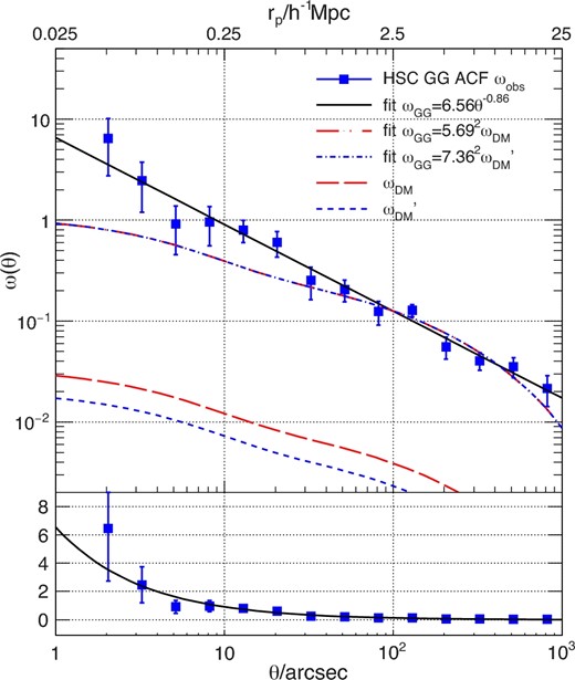
Blue squares are the observed mean ACF ωobs of the LBGs at z ∼ 4 derived from the Jackknife resampling. The solid line is the best-fitting power-law model on the scale 10|${^{\prime\prime}_{.}}$|0 to 1000|${^{\prime\prime}_{.}}$|0. The red dash–dotted line is the best-fitting dark matter model ωDM (red long-dashed line) in the same scale based on the HALOFIT power spectrum (Smith et al. 2003) following the method in Myers et al. (2007), while the blue dash–dotted line is the best-fitting dark matter model |$\omega _{\rm DM}^{\prime }$| (blue short-dashed line) after considering the contamination of the LBGs. The χ2 fitting results are shown. Top and bottom panels show the logarithmic and the linear scale of the vertical axis, respectively. The top horizontal axis of the top panel is the comoving distance at redshift 4. (Color online)
HSC LBG ACF at z ∼ 4.
| θ (″) | (θmin, θmax) | 〈DD〉 | 〈DR〉 | |$\overline{\omega _{i}(\theta )}$| | σ(θ) | θ (″) | (θmin, θmax) | 〈DD〉 | 〈DR〉 | |$\overline{\omega _{i}(\theta )}$| | σ(θ) |
|---|---|---|---|---|---|---|---|---|---|---|---|
| 2.05 | (1.58, 2.51) | 16 | 25 | 6.45 | 3.70 | 51.45 | (39.81, 63.10) | 966 | 9376 | 0.21 | 0.05 |
| 3.25 | (2.51, 3.98) | 16 | 54 | 2.47 | 1.27 | 81.55 | (63.10, 100.00) | 2211 | 22983 | 0.12 | 0.03 |
| 5.15 | (3.98, 6.31) | 20 | 122 | 0.92 | 0.46 | 129.24 | (100.00, 158.49) | 5413 | 56115 | 0.13 | 0.02 |
| 8.15 | (6.31, 10.00) | 48 | 285 | 0.96 | 0.40 | 204.84 | (158.49, 251.19) | 12542 | 138926 | 0.06 | 0.01 |
| 12.92 | (10.00, 15.85) | 105 | 683 | 0.80 | 0.20 | 324.65 | (251.19, 398.11) | 30387 | 341510 | 0.04 | 0.01 |
| 20.48 | (15.85, 25.12) | 219 | 1601 | 0.60 | 0.17 | 514.53 | (398.11, 630.96) | 74669 | 843464 | 0.04 | 0.008 |
| 32.46 | (25.12, 39.81) | 410 | 3833 | 0.25 | 0.90 | 815.48 | (630.96, 1000.0) | 181116 | 2070430 | 0.02 | 0.007 |
Thanks to the large sample of the LBGs, the LBG–LBG pair count is large enough to constrain the ACF even in the smallest bin. We adopt the Jackknife error, which has a value two times larger than the Poisson error at all bins. Most of the bins have clustering signals greater than 3σ.
We fit the raw LBG ACF with a single power-law model ω(θ) = Aωθ−β − IC by χ2 minimization on the scale from 10|${^{\prime\prime}_{.}}$|0 to 1000|${^{\prime\prime}_{.}}$|0. The integral constraint is negligible. Thanks to the small uncertainty of the LBG ACF, the power-law index can be constrained tightly to be |$\beta =0.86^{+0.07}_{-0.06}$| as shown in figure 8. As already mentioned in subsection 3.1, we adopt this power-law index throughout this paper. The best-fitting parameters are listed in table 4.
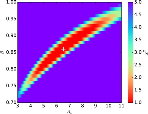
χ2 map of Aω and β parameter of the ACF of the LBGs. The white cross indicates the best-fitting Aω and β at the minimal χ2, while the red region indicates the 68% confidence region. (Color online)
Summary of the clustering analysis of HSC LBGs ACF.
| Model* | Fitting | |$\bar{z}$| | [θmin, θmax] | β | A ω | r 0 | Bias | |
|---|---|---|---|---|---|---|---|---|
| (″) | (h−1 Mpc) | |||||||
| Power-law | χ2 | 3.71 | [10, 1000] | |$0.86^{+0.07}_{-0.06}$| | |$6.56^{+0.49}_{-0.49}$| | |$7.47^{+0.29}_{-0.31}$| | |$5.76^{+0.21}_{-0.22}$| | |
| LBG | Power-law΄ | χ2 | 3.71 | [10, 1000] | |$0.86^{+0.07}_{-0.06}$| | |$10.97^{+0.82}_{-0.82}$| | |$9.85^{+0.39}_{-0.40}$| | |$7.45^{+0.27}_{-0.28}$| |
| ACF | DM | χ2 | 3.71 | [10, 1000] | — | — | — | |$5.69^{+0.21}_{-0.22}$| |
| DM΄ | χ2 | 3.71 | [10, 1000] | — | — | — | |$7.36^{+0.27}_{-0.28}$| |
*The prime symbol indicates models that consider the contamination of the LBG sample.
4 Discussion
4.1 Clustering bias from the correlation length
The measurement of r0 is sensitive to the assumed redshift distribution of the sample. For example, r0 will be smaller if we assume a narrower redshift distribution even for the same Aω. As discussed in subsection 2.4, the redshift distribution of the LBGs is estimated to be more extended than both of the less-luminous and luminous quasar samples. If we assume the redshift distribution of the LBGs is the same as the less-luminous quasars, r0 of the LBG and the less-luminous quasars decreases to |$5.52^{+0.77}_{-0.87}\:h^{-1}\:$|Mpc, which is 23% lower than that estimated originally, because the fraction of the LBGs contributing to the projected correlation function in the overlapped redshift range increases, yielding a weaker correlation strength, i.e., a smaller r0 from a fixed Aω.
4.2 Bias factor from comparing with the HALOFIT power spectrum
In the scale below 10|${^{\prime\prime}_{.}}$|0, the underlying dark matter model becomes flat since we do not consider the one-halo term. If we compare the observed correlation functions with the best-fitting power-spectrum models, there is an obvious overdensity of galaxies on that scale in figure 7, which is consistent with the one-halo term of the LBG ACF at z ∼ 4 (e.g., Ouchi et al. 2005). The left-hand panel of figure 6, also shows an overdensity of galaxies within 10|${^{\prime\prime}_{.}}$|0 around the less-luminous quasars although the error bar is large. Interestingly, we find that the luminous quasars show a deficit of pair count within 10|${^{\prime\prime}_{.}}$|0 in the right-hand panel of figure 6. It should be noted that the best-fitting model in scales larger than 10|${^{\prime\prime}_{.}}$|0 suggests only 1 SDSS quasar–HSC LBG pair within 10|${^{\prime\prime}_{.}}$|0, which is consistent with the deficit. Thus the deficit in small scales can be caused by the limited size of the SDSS quasar sample, though we cannot exclude the possibility that there is a real deficit of galaxies around luminous quasars within 10|${^{\prime\prime}_{.}}$|0.
We consider the contamination by modifying the redshift distribution normalization |$\int _{0}^{\infty }N(z)dz\sim 1-f_{c}$| for the less-luminous quasars and the LBGs. We simply assume that the contamination will not contribute to the underlying dark matter correlation function. The modified underlying dark matter correlation functions are plotted in figures 6 and 7. Since the redshift distribution form is the same after considering the contamination, only the amplitude of the underlying dark matter correlation function is changed. The bias factors with contamination are listed in tables 2 and 4, and are consistent with those derived from fitting with the power-law model after correcting for the contamination.
4.3 Redshift and luminosity dependence of the bias factor
At first, we discuss the luminosity dependence of the bias factors of the luminous and less-luminous quasars in this work. The bias factor of the less-luminous quasars is |$5.93^{+1.34}_{-1.43}$|, which is derived by fitting the CCF with the underlying dark matter model on the scale from 10|${^{\prime\prime}_{.}}$|0 to 1000|${^{\prime\prime}_{.}}$|0 through the ML fitting. The bias factor is consistent with that of the luminous quasars, |$2.73^{+2.44}_{-2.55}$|, obtained from the CCF through the same method within the 1σ uncertainty. If we consider the possible effect of the contamination, the bias factor of the less-luminous quasars increases to |$6.58^{+1.49}_{-1.58}$|, which is still consistent with that of the luminous quasars within the uncertainty. Thus no or only a weak luminosity dependence of the quasar clustering is detected within the two samples.
In order to discuss the redshift dependence of the quasar clustering, we compare the bias factors and those in the literature in the left-hand panel of figure 9. The bias factors in the previous studies show a trend that quasars at higher redshifts are more strongly biased, indicating that quasars preferentially reside in DMHs within a mass range of 1012 ∼ 1013 h−1 M⊙ from z ∼ 0 to z ∼ 4. There is no discrepancy between the bias factors estimated with the ACF and the CCF at z ≲ 3. In this work, the bias factor of the less-luminous quasars at z ∼ 4 follows the trend, while the bias factor of the luminous quasars is similar to or even smaller than those at z ∼ 3.
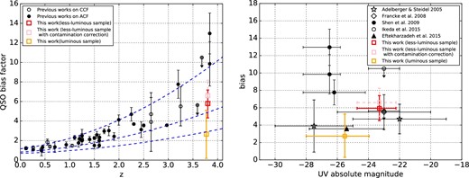
Left-hand panel: Redshift evolution of the quasar bias factor. The red square is the result from fitting the less-luminous quasar CCF against the underlying dark matter model through ML fitting. The pink square is derived from fitting the less-luminous quasar CCF with the same method after considering the contamination. The orange square is obtained from fitting the luminous quasar CCF with the same method. Open and filled black circles are bias factors of quasars in a wide luminosity range obtained from the CCF and the ACF, respectively, in the literature, which are summarized by Ikeda et al. (2015) and Eftekharzadeh et al. (2015). Blue dashed lines show the bias evolutions of halos with a fixed mass of 1011, 1012, and 1013 h−1 M⊙ from bottom to top following the fitting formulae in Sheth, Mo, and Tormen (2001). Right-hand panel: Luminosity dependence of the quasar bias at 3 < z < 5. Red and orange squares have the same meaning as in the left-hand panel. The stars, diamonds, dots, triangle, open circles and squares are from Adelberger and Steidel (2005), Francke et al. (2007), Shen et al. (2009), Eftekharzadeh et al. (2015), Ikeda et al. (2015), and this work, respectively. Open and filled symbols imply the bias factors derived from the CCF and ACF, respectively. (Color online)
The luminosity dependence of the quasar bias factors at z ∼ 3–4 is summarized in the right-hand panel of figure 9. Both of the bias factors of the less-luminous quasars with and without the contamination correction are consistent with but slightly higher than that evaluated with the CCF of 54 faint quasars in the magnitude range of −25.0 < MUV < −19.0 at 1.6 < z < 3.7 measured by Adelberger and Steidel (2005), the CCF of 58 faint quasars in the magnitude range of −26.0 < MUV < −20.0 at 2.8 < z < 3.8 measured by Francke et al. (2007), and the CCF of 25 faint quasars in the magnitude range of −24.0 < MUV < −22.0 at 3.1 < z < 4.5 measured by Ikeda et al. (2015), which suggests a slightly increasing or no evolution from z = 3 to z = 4.
Meanwhile, for the clustering of the luminous quasars, the bias factor in this work is consistent with the CCF of 25 bright quasars in the magnitude range of −30.0 < MUV < −25.0 at 1.6 < z < 3.7 measured by Adelberger and Steidel (2005) and the ACF of 24724 bright quasars in the magnitude range of −27.81 < MUV < −22.9 mag at 2.64 < z < 3.4 measured by Eftekharzadeh et al. (2015). Unlike the case of the less-luminous quasars, the clustering of the luminous quasars suggests no or a declining evolution from z ∼ 3 to z ∼ 4. The bias factor of the luminous quasars in this work shows a large discrepancy with the ACF of 1788 bright quasars in the magnitude range of −28.2 < MUV < −25.8 [which is transferred from Mi(z = 2) by equation (3) in Richards et al. (2006)] at 3.5 < z < 5.0 measured by Shen et al. (2009). They give two values for the bias factor; the higher one is obtained by only considering the positive bins and the lower one considers all of the bins in the ACF. The bias factor from another subsample of bright quasars covering −28.0 < MUV < −23.95 at 2.9 < z < 3.5 in Shen et al. (2009) is also shown in the panel.
The z ∼ 4 quasar bias factors in Shen et al. (2009) show a large discrepancy from the bias factor of the luminous quasars in this work and in Eftekharzadeh et al. (2015) with the similar magnitude and redshift coverage. In the right-hand panel of figure 6, we plot the expected CCF with |$b_{\rm QG}\sim \sqrt{b_{\rm QSO}b_{\rm LBG}}=9.83$| by the orange dash–double-dotted line. We adopt the higher bQSO in Shen et al. (2009) and the bLBG with the contamination correction to measure the upper limit of the bQG. Although the expected CCF is consistent with some bins within the 1σ uncertainty, it predicts much stronger clustering than both of the best-fitting power-law and dark matter models. In order to quantitatively examine the discrepancy, we plot the minimization function S of the ML fitting for the luminous quasars with the HALOFIT power spectrum as a function of the bias factor in figure 10. Both of the bias factors at 3.5 < z < 5 in Shen et al. (2009) are beyond the 1σ uncertainty, corresponding to a low probability. Meanwhile, the bias factor in Eftekharzadeh et al. (2015), the uncertainty of which is small thanks to the large sample, also shows a large discrepancy from those in Shen et al. (2009). Eftekharzadeh et al. (2015) suspect the discrepancy is mainly caused by a difference in large scale bins (>30 h−1 Mpc). We further investigate the effect from the fitting scale as shown in table 1 and the right-hand panel of figure 6. On a scale of 40|${^{\prime\prime}_{.}}$|0 to 160|${^{\prime\prime}_{.}}$|0, we find a strong CCF of the luminous quasars and the LBGs, which is consistent with the ACF of the luminous quasars. On scales below 40|${^{\prime\prime}_{.}}$|0, the ML fitting suggests a bQG of 0. On larger scales, the ML fitting is not efficient since the pair counts in each bin is too large to fulfil the assumption that bins are independent of each other, even if choosing a small bin width of 0|${^{\prime\prime}_{.}}$|5 interval. Therefore we only expand the ML fitting scale to 2000|${^{\prime\prime}_{.}}$|0. If we consider the power-law model, the bQG obtained by fitting in the range of 40|${^{\prime\prime}_{.}}$|0 to 1000|${^{\prime\prime}_{.}}$|0 is 24.7% and 7.6% higher than that estimated in the range of 10|${^{\prime\prime}_{.}}$|0 to 1000|${^{\prime\prime}_{.}}$|0 and of 40|${^{\prime\prime}_{.}}$|0 to 2000|${^{\prime\prime}_{.}}$|0, respectively, which suggests that the deficit of the luminous quasar–LBG pair on small scales may weaken the CCF more severely than fitting on scales larger than 1000|${^{\prime\prime}_{.}}$|0. Here, since the fitting of the luminous quasar CCF strongly depends on the scale, especially on small scales, we still focus on the results on the scale from 10|${^{\prime\prime}_{.}}$|0 to 1000|${^{\prime\prime}_{.}}$|0 to keep accordant to the LBG ACF and the less-luminous quasar CCF throughout the discussion.
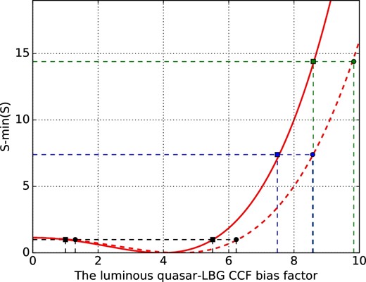
ML fitting minimization function S of fitting for the luminous quasar CCF with the dark matter model. S is shown in relative to the minimal value. Black squares mark the 68% upper and lower limits of bQG with S − min(S) = 1. Blue and green squares indicate the expected bias factors of |$b_{\,\rm QG}\sim \sqrt{b_{\,\rm QSO}b_{\,\rm LBG}}=7.53$| and 8.64 from the bias factors of the SDSS luminous quasars in Shen et al. (2009) with and without considering the negative bins in the ACF, respectively. The red dashed line indicates the same minimization function S after considering the possible contamination in the LBG sample. Black, blue and green dots have the same meaning as the squares. (Color online)
Quasar clustering models based on numerical simulation predict no luminosity dependence of the quasar clustering at z ∼ 4 (e.g., Fanidakis et al. 2013; Oogi et al. 2016; DeGraf & Sijacki 2017). Although there is a relation between mass of the SMBHs and DMHs in the models, SMBHs in a wide mass range are contributing to quasars at a fixed luminosity, thus there is no relation between the luminosity of model quasars and the mass of their DMHs. Oogi et al. (2016) and DeGraf and Sijacki (2017) predicted a quasar bias factor of ∼5.0 at redshift 4, which is consistent with the quasar bias factors in this work. No luminosity dependence is also predicted in a continuous SMBH growth model of Hopkins et al. (2007). They assume an Eddington limited SMBH growth until redshift 2. However, the predicted bias factor is much larger than the results in this work. On the other hand, there are models which predict stronger luminosity dependence of the quasar clustering at higher redshifts (e.g., Shen 2009; Conroy & White 2012). These models predict that SMBHs in a narrow mass range are contributing to the luminous quasars.
In order to conclude the luminosity and redshift dependencies of the quasar clustering, we need to understand the cause of the discrepancy between the quasar ACF and quasar–LBG CCF for the luminous quasars at z ∼ 4. The quasar–LBG CCF could be affected by the suppression of galaxy formation due to feedback from luminous quasars (e.g., Kashikawa et al. 2007; Utsumi et al. 2010; Uchiyama et al. 2018). The weak cross-correlation could also be induced by a discrepancy between the redshift distributions of the quasars and LBGs. We need to further determine the redshift distribution through spectroscopic follow-up observations of the LBGs.
4.4 Effect of edge regions and seeing variation on the bias factor
It should be noted that there is a sky coverage discrepancy between the samples of the quasars and LBG candidates in the shallower edge regions. As a result, it is possible that most of the 〈DQSODLBG〉 pair counts on small scales are from quasars only in inner regions, which may cause the weakness of the small-scale clustering between the luminous quasars and LBGs, if the random LBG sample cannot reproduce the detection completeness in the edge regions. Although we have mentioned that our random LBGs can reproduce the overall distribution of the real LBGs in subsection 2.5, to evaluate the effects quantitatively we select the central area in each subregion to construct a subsample of less-luminous quasars, luminous quasars, LBGs, and random LBGs. We apply the same estimator as in section 3.1 to measure their correlation functions. We fit a single power-law to the resulting ACF and CCF, then compare them to that of the original samples. Poisson error is adopted here for simplicity.
In table 5, we summarize bQG and bLBG obtained from the samples in the inner (“No” in the border column) and entire regions (“Yes” in the border column). For the LBG ACF on the scale below 1000|${^{\prime\prime}_{.}}$|0 and less-luminous quasar CCF beyond 15|${^{\prime\prime}_{.}}$|0, they do not have a significant discrepancy from that of the entire samples except for a larger uncertainty, and the size of luminous quasar subsample is too limited to judge the border effect. On the scale below 15|${^{\prime\prime}_{.}}$|0, we find bQG of the subsamples is enhanced from |$7.48^{+1.39}_{-1.68}$| to |$10.61^{+2.29}_{-2.88}$|. Since the uncertainty is large due to the limited size of pair counts on small scales, we could not make a conclusion whether the deficit of luminous quasar - LBG pair counts in scale within 15|${^{\prime\prime}_{.}}$|0 is due to the effect of the border regions or real.
Clustering dependence on the border and seeing.
| Model | Fitting | Border | Seeing | [θmin, θmax] | Bias | |
|---|---|---|---|---|---|---|
| (″) | ||||||
| Power-law | χ2 | Yes | All | [10, 1000] | |$5.64^{+0.56}_{-0.62}$| | |
| Less- | Power-law | χ2 | No | All | [15, 1000] | |$6.15^{+0.75}_{-0.85}$| |
| lumiNous QG | Power-law | χ2 | Yes | All | [3, 15] | |$7.48^{+1.39}_{-1.68}$| |
| CCF | Power-law | χ2 | No | All | [3, 15] | |$10.61^{+2.29}_{-2.88}$| |
| Power-law | χ2 | Yes | [0|${^{\prime\prime}_{.}}$|5, 0|${^{\prime\prime}_{.}}$|7] | [10, 1000] | |$5.37^{+0.68}_{-0.78}$| | |
| Power-law | χ2 | Yes | All | [3, 1000] | |$5.69^{+0.13}_{-0.13}$| | |
| LBG | Power-law | χ2 | No | All | [3, 1000] | |$5.55^{+0.18}_{-0.18}$| |
| ACF | Power-law | χ2 | Yes | [0|${^{\prime\prime}_{.}}$|5, 0|${^{\prime\prime}_{.}}$|7] | [3, 1000] | |$5.40^{+0.16}_{-0.16}$| |
Another problem that can affect the clustering analysis is the variation of detection completeness due to non-uniform seeing distribution within the Wide layer dataset. In subsection 2.5, we confirmed the random LBGs can reproduce the seeing dependence of the detection completeness of the real LBGs. Here, we quantitatively investigate the influence from the seeing variation by constructing a uniform subsample of less-luminous quasars, LBGs and random LBGs taken under seeing between 0|${^{\prime\prime}_{.}}$|5 and 0|${^{\prime\prime}_{.}}$|7. The same estimator as in subsection 3.1 and Poisson error are adopted to measure their correlation functions. In table 5, we summarize bQG and bLBG obtained with the seeing limited and entire samples. Compared to the correlation functions of the entire samples, there is no significant discrepancy of both of the less-luminous quasar CCF and LBG ACF of the seeing-limited samples except for larger uncertainty, which again suggests the seeing variation does not affect the results of the clustering.
4.5 DMH mass
Assuming the quasars and LBGs are associated with DMHs in a narrow mass range, we can infer the mass of the quasar host DMHs through the above relations. The evaluated halo masses of the less-luminous quasars and the luminous quasars are 1 ∼ 2 × 10¹² h−1 M⊙ and <1012 h−1 M⊙ as summarized in table 2, respectively. Since the bias factor of the luminous quasars has a large uncertainty, we could only set an upper limit of the MDMH. We note that the halo mass strongly depends on the amplitude of the power spectrum on the scale of 8 h−1 Mpc, σ8. If we adopt σ8 = 0.9, the host DMH mass of the less-luminous quasars will be 4–6 × 10¹² h−1 M⊙ with the same bias factor.
4.6 Minimum halo mass and duty cycle
We compare the duty cycles with those evaluated for quasars at 2 < z < 4 in the literature in figure 11. The estimated luminosity dependence of the duty cycles is similar to that estimated for quasars in the similar luminosity range at z ∼ 2.6 (Adelberger & Steidel 2005), although the duty cycles at z ∼ 4 are one order of magnitude smaller than those at z ∼ 2.6.
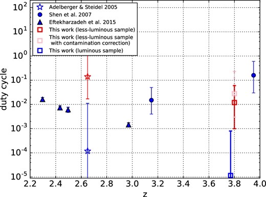
Estimated quasar duty cycle as a function of redshift. The blue symbols represent the duty cycles estimated with a sample of quasars mostly with MUV < −25. The red symbols show those for the less-luminous quasars with MUV > −25. Stars, triangles, filled circles and squares represent the results from Adelberger and Steidel (2005), Shen et al. (2007), Eftekharzadeh et al. (2015), and this work. The pink open square shows the duty cycle with the contamination correction. (Color online)
The estimated duty cycle corresponds to a duration of the less-luminous quasar activity of 1.5–90.8 Myr, which is broadly consistent with the quasar lifetime range of 1–100 Myr estimated in previous studies (for review see Martini 2004). It needs to be noted that the estimated duty cycle is sensitive to the measured strength of the quasar clustering. A small variation in the bias factor can result in even one order of magnitude difference in the duty cycle, because of the non-linear relation between b and MDMH and the sharp cut-off of n(M) at the high-mass end. Furthermore, the duty cycle is also sensitive to the assumed value of σ8 (Shen et al. 2007).
5 Summary
We examine the clustering of a sample of 901 less-luminous quasars with −24.73 < M1450 < −22.23 at 3.1 < z < 4.6 selected from the HSC S16A Wide2 catalog and of a sample of 342 luminous quasars with −28.00 < M1450 < −23.95 at 3.4 < zspec < 4.6 within the HSC S16A Wide2 coverage from the 12th data release of SDSS. We investigate the quasar clustering through the CCF between the quasars and a sample of 25790 bright LBGs with M1450 < −21.25 in the same redshift range from the HSC S16A Wide2 data release. The main results are as follows.
1. The bias factor of the less-luminous quasar is |$5.93^{+1.34}_{-1.43}$| derived by fitting the CCF with the dark matter power-spectrum model through the ML method, while that of the luminous quasars is |$2.73^{+2.44}_{-2.55}$| obtained in the same manner. If we consider the contamination rates of 22.7% and 10.0% estimated for the LBG and the less-luminous quasar samples, respectively, the bias factor of the less-luminous quasars can increase to |$6.58^{+1.49}_{-1.58}$| on the assumption that the contaminating objects are distributed randomly.
2. The CCFs of the luminous and less-luminous quasars do not show significant luminosity dependence of the quasar clustering. The bias factor of the less-luminous quasars suggests that the environment around them is similar to the luminous LBGs used in this study. The luminous quasars do not show strong association with the luminous LBGs on scales from 10|${^{\prime\prime}_{.}}$|0 to 1000|${^{\prime\prime}_{.}}$|0, especially on scales smaller than 40|${^{\prime\prime}_{.}}$|0. The bias factor of the luminous quasar is smaller than that derived from the ACF of the SDSS quasars at z ∼ 4 (Shen et al. 2009). The reason may be partly due to the deficit of the pairs on small scales, which can be caused by the border between quasar and LBG samples at shallower edge regions or by a physical mechanism, e.g., the strong feedback from the SMBH.
3. The bias factor of the less-luminous quasars corresponds to a mass of DMHs of ∼1–2 × 10¹² h−1 M⊙. Minimal host DMH mass for the quasars can be also inferred from the bias factor. Combining the halo number density above that mass threshold and the observed quasar number density, the fraction of halos which are in the less-luminous quasar phase is estimated to be 0.001–0.06 from the CCF. The corresponding quasar lifetime is 1.5–90.8 Myr.
Correlation analysis in this work is conducted in the projected plane, and accurate information on the redshift distribution of the samples and the contamination rates is necessary to obtain reliable constraints on the clustering of the z ∼ 4 quasars. Spectroscopic follow-up observations are expected to obtain the accurate information. Additionally, the full HSC Wide survey plans to cover 1400 deg2 in 5 years, which can significantly enhance the sample size. The statistical significance of the current results can then be largely improved.
Acknowledgements
We would like to thank the valuable comments from the referee. We also would like to thank Dr. A.K. Inoue who kindly provides us with the IGM model data.
The Hyper Suprime-Cam (HSC) collaboration includes the astronomical communities of Japan and Taiwan, and Princeton University. The HSC instrumentation and software were developed by the National Astronomical Observatory of Japan (NAOJ), the Kavli Institute for the Physics and Mathematics of the Universe (Kavli IPMU), the University of Tokyo, the High Energy Accelerator Research Organization (KEK), the Academia Sinica Institute for Astronomy and Astrophysics in Taiwan (ASIAA), and Princeton University. Funding was contributed by the FIRST program from Japanese Cabinet Office, the Ministry of Education, Culture, Sports, Science and Technology (MEXT), the Japan Society for the Promotion of Science (JSPS), Japan Science and Technology Agency (JST), the Toray Science Foundation, NAOJ, Kavli IPMU, KEK, ASIAA, and Princeton University.
Funding for the Sloan Digital Sky Survey IV has been provided by the Alfred P. Sloan Foundation, the U.S. Department of Energy Office of Science, and the Participating Institutions. SDSS-IV acknowledges support and resources from the Center for High-Performance Computing at the University of Utah. The SDSS web site is 〈www.sdss.org〉.
SDSS-IV is managed by the Astrophysical Research Consortium for the Participating Institutions of the SDSS Collaboration including the Brazilian Participation Group, the Carnegie Institution for Science, Carnegie Mellon University, the Chilean Participation Group, the French Participation Group, Harvard-Smithsonian Center for Astrophysics, Instituto de Astrofísica de Canarias, The Johns Hopkins University, Kavli Institute for the Physics and Mathematics of the Universe (IPMU)/University of Tokyo, Lawrence Berkeley National Laboratory, the Leibniz Institut für Astrophysik Potsdam (AIP), the Max-Planck-Institut für Astronomie (MPIA Heidelberg), the Max-Planck-Institut für Astrophysik (MPA Garching), the Max-Planck-Institut für Extraterrestrische Physik (MPE), the National Astronomical Observatories of China, New Mexico State University, New York University, the University of Notre Dame, Observatário Nacional / MCTI, The Ohio State University, Pennsylvania State University, Shanghai Astronomical Observatory, the United Kingdom Participation Group, Universidad Nacional Autónoma de México, the University of Arizona,the University of Colorado Boulder, the University of Oxford, the University of Portsmouth, the University of Utah, the University of Virginia, the University of Washington, the University of Wisconsin, Vanderbilt University, and Yale University.
This paper makes use of software developed for the Large Synoptic Survey Telescope. We thank the LSST Project for making their code available as free software at 〈http://dm.lsst.org〉.
The Pan-STARRS1 Surveys (PS1) have been made possible through contributions of the Institute for Astronomy, the University of Hawaii, the Pan-STARRS Project Office, the Max-Planck Society and its participating institutes, the Max Planck Institute for Astronomy, Heidelberg and the Max Planck Institute for Extraterrestrial Physics, Garching, The Johns Hopkins University, Durham University, the University of Edinburgh, Queen’s University Belfast, the Harvard-Smithsonian Center for Astrophysics, the Las Cumbres Observatory Global Telescope Network Incorporated, the National Central University of Taiwan, the Space Telescope Science Institute, the National Aeronautics and Space Administration under Grant No. NNX08AR22G issued through the Planetary Science Division of the NASA Science Mission Directorate, the National Science Foundation under Grant No. AST-1238877, the University of Maryland, and Eotvos Lorand University (ELTE).
References
