


Abstract
We present the cross-correlation between 151 luminous quasars (MUV < −26) and 179 protocluster candidates at z ∼ 3.8, extracted from the Wide imaging survey (∼121 deg2) performed as part of the Hyper Suprime-Cam Subaru Strategic Program (HSC-SSP). We find that only two out of 151 quasars reside in regions that are more overdense compared to the average field at >4 σ. The distributions of the distances between quasars and the nearest protoclusters and the significance of the overdensity at the positions of quasars are statistically identical to those found for g-dropout galaxies, suggesting that quasars tend to reside in almost the same environment as star-forming galaxies at this redshift. Using stacking analysis, we find that the average density of g-dropout galaxies around quasars is slightly higher than that around g-dropout galaxies on 1.0–2.5 pMpc scales, while at <0.5 pMpc that around quasars tends to be lower. We also find that quasars with higher UV luminosity or with more massive black holes tend to avoid the most overdense regions, and that the quasar near-zone sizes are anti-correlated with overdensity. These findings are consistent with a scenario in which luminous quasars at z ∼ 4 reside in structures that are less massive than those expected for the progenitors of today’s rich clusters of galaxies, and possibly that luminous quasars may be suppressing star formation in their close vicinity.
1 Introduction
Quasars are among the most luminous objects in the Universe, and their luminosity is powered by accretion onto supermassive black holes (SMBHs) in the center of their host galaxies. The descendants of the most luminous quasars which have higher black hole mass likely reside in massive dark halos (Shen et al. 2007) and host galaxies today, according to the M–σ relation (Magorrian et al. 1998; Marconi & Hunt 2003). At high redshift, the reservoir of gas feeding the quasars can be supplied by cold streams (e.g., Kereš et al. 2005; Dekel & Birnboim 2006; Ocvirk et al. 2008) or major (wet) mergers (e.g., Lin et al. 2008). This suggests that the activity of quasars, and therefore their SMBH growth, may depend not only on their intrinsic properties but also on the surrounding environment beyond the scale of a galaxy. However, it is not known how exactly the large-scale environment affects the mass accretion onto an SMBH whose scale is much smaller than that of a galaxy.
It is generally assumed that the most luminous quasars and galaxies are hosted by massive halos (Springel et al. 2005). Therefore, if quasar activity is triggered by frequent mergers or cold streams, it should preferentially occur in the peaks of the matter density field, which are rare (Hopkins et al. 2008). Accordingly, quasars have been thought to act as signposts for high-redshift protoclusters (or clusters in formation), which are thought to evolve into the galaxy clusters seen in the local Universe. For example, Husband et al. (2013) found that three luminous quasars at z ∼ 5 reside in overdense regions of Lyman break galaxies (LBGs). Morselli et al. (2014) found more i-dropout galaxies in four z ∼ 6 quasar fields than expected in a blank field. Adams et al. (2015) reported that about 10%
of a sample of luminous quasars at z ∼ 4 reside in overdense regions of Lyα emitters (LAEs). Bañados et al. (2013) and Mazzucchelli et al. (2017) used deep narrow- and broad-band imaging to study the environment of z ∼ 5.7 quasars, and found no enhancement of LAEs compared with average fields, implying either high-z quasars may not trace the most massive dark matter halos, or the strong radiation from the quasar may be suppressing star formation in galaxies in its immediate vicinity (Kashikawa et al. 2007; Bruns et al. 2012, and see subsection 4.2). Kim et al. (2009) concluded that only two fields were overdense among five quasar fields at z ∼ 6. Trainor and Steidel (2012) showed that hyper-luminous quasars reside in galaxy overdense regions, but the environment around them is not very different from that around much less luminous quasars. Angulo et al. (2012) showed that the z = 0 descendant halo masses of z ∼ 6 quasars widely span from cluster- to group-scale masses even if the quasars reside in the most massive objects at that time, based on a cosmological N-body simulation. Recently, Kikuta et al. (2017) investigated quasar fields at z ∼ 4.9 to suggest that high-z quasars are not associated with extreme galaxy overdense regions. From the above, it is clear that a consistent picture of the environment of high-z quasars still needs to be derived (for a review, see Overzier 2016).
The underlying dark halo masses of quasar hosts have been statistically estimated by clustering analysis. The optically selected quasar halo masses at z ∼ 1–3 are consistent with the typical halo mass of ∼1012 M⊙ at that epoch (Adelberger & Steidel 2005; Coil et al. 2007; White et al. 2012), suggesting they do not reside in very biased regions. In fact, recently, Cai et al. (2016) found that the masses of protoclusters which are traced by Lyα forest absorption are much more massive than those of typical quasars at z ∼ 2–3. At higher redshift z > 3, Shen et al. (2007) showed that optical quasar halo masses are more massive with M ∼ (4–6) × 1012 h−1 M⊙ , implying that almost all luminous quasars could be associated with cluster progenitors. On the other hand, Fanidakis et al. (2013) used GALFORM (Cole et al. 2000; Fanidakis et al. 2012; Lacey et al. 2015), a semi-analytic model that takes into account active galactic nuclei (AGN) feedback suppressing gas cooling in massive halos, to conclude that typical quasars reside in halos whose average masses are ∼1011.5–1012 h−1 M⊙ at z > 3; therefore they are not typically hosted by the most massive halos or the progenitors of the most massive local clusters. According to GALFORM, the quasar halo masses are regulated by AGN feedback; the most massive halos are in the state in which SMBH mass and spin are higher and the accretion rate is lower due to radio mode feedback compared to the less massive halos. As a result, it is difficult for quasars to appear in the most massive halos. Recently, Oogi et al. (2016) used νGC, which is another semi-analytic model of galaxy and quasar formation (Enoki et al. 2003, 2014; Nagashima et al. 2005; Shirakata et al. 2015), to estimate median quasar halo masses of a few 1011 M⊙ at z = 4. These predicted average quasar halo masses are much smaller than expected for progenitors of local clusters, and as a consequence, they imply that quasars should not typically be associated with galaxy overdensities at high redshift. However, until now, good empirical data on high-z quasar environments, and especially the relation between quasar activity and overdense regions, has been lacking.
Until recently, the number of known protoclusters at z > 3 has been small, ∼10 (Chiang et al. 2013). This means it has been difficult to systematically examine the relation between quasars and their environments. A direct technique to detect nearby clusters by looking for the thermal X-ray emission from the intra-cluster medium (Böhringer et al. 2001) is insensitive at z > 2, where clusters are expected to be in the growing phase. In order to overcome this problem, we have utilized Hyper Suprime-Cam (HSC: Miyazaki et al. 2012), which is an unprecedented wide-field imaging instrument mounted on the 8.2 m Subaru telescope, to build the largest sample of z ∼ 4 protoclusters to date (Toshikawa et al. 2018). The new protocluster sample was derived from data from the Strategic Program for the Subaru Telescope (HSC-SSP: P.I. S. Miyazaki), which is currently ongoing (Tanaka et al. 2018). Our bias-free wide-field protocluster survey allows us to also investigate the general relationship between quasars and protoclusters, which will help to understand the early interplay between structure formation and galaxy and SMBH co-evolution. In this paper, we used the first release data (DR1) of HSC-SSP of ∼121 square degrees to statistically characterize the environment of a large number of optically selected quasars at z ∼ 3.8 from the Sloan Digital Sky Survey (SDSS), by measuring their typical environmental density and the cross-correlation with our protocluster catalog at the same redshift.
This paper is organized as follows. In section 2, we describe the protocluster sample in the HSC-Wide layer, and our SDSS quasar sample. In section 3, we investigate the correlation between protoclusters and quasars, and discuss whether or not quasars are statistically good indicators of protoclusters. We further examine the average radial density profile around quasars on the small scale using a stacking analysis, and its dependence on quasar luminosity and black hole mass. The implications of our results are discussed in section 4. Finally, in section 5 we conclude and summarize our findings. We assume the following cosmological parameters: ΩM = 0.3, ΩΛ = 0.7, H0 = 70 km s−1 Mpc−1, and magnitudes are given in the AB system.
2 Data and sample selection
2.1 The Subaru HSC-SSP survey
The Subaru HSC-SSP survey started in early 2014, and will spend 300 nights until completion by 2019 or 2020. HSC is equipped with 116 2 K × 4 K Hamamatsu fully depleted CCDs, of which 104 CCDs are used to obtain science data over a field of view of 1|${^{\circ}_{.}}$|5 diameter. The present paper is based on the so-called Wide layer of the HSC-SSP, which has wide-area coverage (in the future, the survey area will reach ∼1400 deg2) and high sensitivity through five optical (g, r, i, z, y) bands. The total exposure times range from 10 min in the g and r bands to 20 min in the i, z, and y bands. The expected 5 σ limiting magnitudes for point sources are (g, r, i, z, y) = (26.5, 26.1, 25.9, 25.1, 24.4) mag, measured in 2|${^{\prime\prime}_{.}}$|0 apertures. We expect to obtain >1400 protocluster candidates at z ∼ 4 by the end of the survey (Toshikawa et al. 2016, 2018). The HSC data (DR S16A: Aihara et al. 2018b), which includes data taken before 2016 April, has already produced an extremely wide field image of >200 deg2 with a median seeing of 0|${^{\prime\prime}_{.}}$|6–0|${^{\prime\prime}_{.}}$|8 in the Wide layer. The survey design is shown in Aihara et al. (2018a). The filter information is given in Kawanomoto et al. (2017). Data reduction was performed with the dedicated pipeline hscPipe (version 4.0.2; Bosch et al. 2018), a modified version of the Large Synoptic Survey Telescope software stack (Ivezic et al. 2008; Axelrod et al. 2010; Jurić et al. 2015). The astrometric and photometric calibrations are associated with the Pan-STARRS1 system (Schlafly et al. 2012; Tonry et al. 2012; Magnier et al. 2013). We use the cModel magnitude, which is measured by fitting two-component, PSF-convolved galaxy models (de Vaucouleurs and exponential) to the source profile (Abazajian et al. 2004). We measure the fluxes and colors of sources with cModel.
2.2 HSC protocluster sample
Our new large survey for high-redshift protoclusters based on the unprecedented imaging data produced by the HSC-SSP survey is ongoing. We use the catalog of protocluster candidates at z ∼ 4 as described in the forthcoming paper, Toshikawa et al. (2018). We briefly review the key steps of the construction of the protocluster catalog here.
Details of the five fields included in the HSC-SSP Data Release S16A used in this analysis.
| Name | Range in RA (J2000.0) | Range in Dec (J2000.0) | Effective area [deg2] |
|---|---|---|---|
| W-XMMLSS | 1h36m00s to 3h00m00s | −6°00΄00″ to −2°00΄00″ | 31.26 |
| W-Wide12H | 11h40m00s to 12h20m00s | −2°00΄00″ to 2°00΄00″ | 17.00 |
| W-GAMA15H | 14h00m00s to 15h00m00s | −2°00΄00″ to 2°00΄00″ | 39.27 |
| W-HECTMAP | 15h00m00s to 17h00m00s | 42°00΄00″ to 45°00΄00″ | 12.60 |
| W-VVDS | 22h00m00s to 23h20m00s | −2°00΄00″ to 3°00΄00″ | 20.73 |
Next, the fixed aperture method was applied to determine the surface density contour maps of g-dropout galaxies. Apertures with a radius of 1|${^{\prime}_{.}}$|8, which corresponds to 0.75 physical Mpc (pMpc) at z ∼ 3.8, were distributed in the sky of the HSC-Wide layer. This aperture size is comparable with the typical protocluster size at this epoch with a descendant halo mass of ≳ 1014 M⊙ at z = 0 (Chiang et al. 2013). To determine the overdensity significance quantitatively, we estimated the local surface number density by counting galaxies within the fixed aperture. The overdensity significance is defined by |$(N -\bar{N})/\sigma$|, where N is the number of g-dropout galaxies in an aperture, and |$\bar{N}$| and σ are the average and standard deviation of N, respectively. Red galaxies at intermediate redshifts and dwarf stars could satisfy our color selection criteria. The fraction of contamination from these objects in the g-dropout color selection is evaluated to be 25% at most at i < 25.0 (Ono et al. 2018), 20% of which originate in photometric error (Toshikawa et al. 2016). The overdensity significance should not be greatly affected by the contamination.
The final protocluster candidates were selected from those regions that had overdensities with >4 σ significance. Although there is a large scatter due to projection effects, surface overdensity significance is closely correlated with descendant halo mass at z = 0. Toshikawa et al. (2016) showed that >76% of >4 σ overdense regions of g-dropouts are expected to evolve into dark matter halos with masses of >1014 M⊙ at z = 0, although there is no clear difference between <4 σ overdense regions and fields due to a large scatter. It should be noted that the success rate of this technique has already been established by our previous study of the ∼4 deg2 of the CFHTLS Deep Fields, as the precursor of this HSC protocluster search, followed by Keck/DEIMOS and Subaru/FOCAS spectroscopy (Toshikawa et al. 2016). We carefully checked each >4 σ overdense region, and removed 22 fake detections of mainly spiral arms of local galaxies. As a result, we find 179 protocluster candidates at z ∼ 3.8 in the HSC-Wide layer having overdensity significance ranging from 4 to 10 σ. Figure 1 shows the histogram of the overdensity significance of the protocluster candidates.

Histogram of overdensity significance of the 179 protocluster candidates from Toshikawa et al. (2018). The horizontal axis shows the significance of the overdensities of g-dropout galaxies measured within 1|${^{\prime}_{.}}$|8 radius circular apertures across the HSC-SSP Wide layer. The maximum significance is 9.37. (Color online)
2.3 Quasars
Our quasar sample was extracted from the Sloan Digital Sky Survey (SDSS) quasar catalog of Pâris et al. (2017) based on SDSS DR12. The SDSS DR12 quasar catalog is the final SDSS-III quasar catalog. It contains 297301 spectroscopically confirmed quasars over a wide redshift range of 0.041 < z < 6.440 in an area covering approximately 10200 deg2 of the sky. The quasars have been selected from three different observational programs: (1) the Baryon Oscillation Spectroscopic Survey (BOSS; Dawson et al. 2013), (2) ancillary programs such as the SDSS-IV pilot survey, and (3) objects targeted by chance in other programs, such as the luminous galaxy survey. For the details of target selection for spectroscopic observation and quasar confirmation, please see Ross et al. (2012). Within the g-dropout redshift range of z = 3.3–4.2, which corresponds to the g-dropout selection function with value over 0.4 (Ono et al. 2018), we find 151 quasars in the effective areas of the HSC-Wide layer used in our analysis. The i-band absolute magnitudes of this sample range from ∼−29 to −26 (see figure 7). We use the reduced one-dimensional (1D) spectral data of the quasars, which are available through the SDSS Science Archive Server (SAS), to estimate the black hole masses for this sample (subsection 3.3). The spectral resolution is R ∼ 1300–2500 (Pâris et al. 2017). If the quasars have a match in the FIRST radio catalog (Becker et al. 1995), whose detection limit is 1 mJy, within 2|${^{\prime\prime}_{.}}$|0, the FIRST_MATCHED flag in the SDSS DR12 catalog is set to 1 (Pâris et al. 2017). The sample contains eight FIRST-detected quasars (FIRST_MATCHED = 1) with strong radio emission of Lν(6.74 GHz) > 5.0 × 1032 erg s−1 Hz−1, which is about 10 times larger than that of a dichotomy between star-forming galaxies and radio-active AGNs (Magliocchetti et al. 2002; Mauch & Sadler 2007). It should be noted that the radio property of an AGN affects the clustering strength (Donoso et al. 2010).
3 Results
3.1 Cross-correlation between protoclusters and quasars
First, we measured the projected distance from the quasars to the nearest protoclusters to determine whether the two populations are related. The results are shown in figure 2. The blue histogram shows the angular separations between quasars and protoclusters, while the orange line shows the separations between g-dropout galaxies and protoclusters. The p-value of the Kolmogorov–Smirnov (KS) test between the two distributions is 0.573, showing that they are not significantly different, at least on these scales. We also focused on the smaller scale < 0|${^{\circ}_{.}}$|2 to conduct a similar analysis (see the small chart in figure 2), but the result did not change: the p-value in the KS test is 0.100.
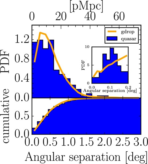
Histogram of distance from quasars and g-dropouts to the nearest protocluster candidates. The blue rods show the case of quasars, and the red line shows the case of all g-dropout galaxies. On the vertical axis we show the probability distribution function (PDF) and the cumulative PDF. The small chart shows the PDF in the region limited to the small scales, <0|${^{\circ}_{.}}$|2. (Color online)
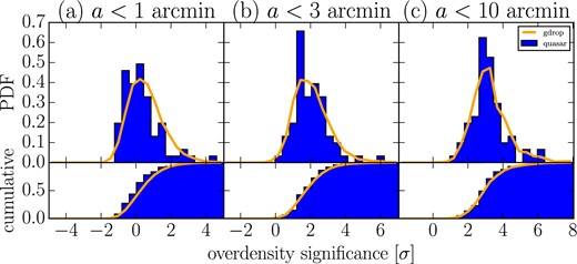
To measure the environments in detail, we also measured the overdensity significances at the exact locations of the quasars. Because it is known that quasars and radio galaxies at these redshift are not always right at the center of the overdense regions (e.g., Venemans et al. 2007), we measured the maximum overdensity significance within a circle of radius a = 1΄ (2.5 comoving Mpc; cMpc). Figure 3 a shows the probability distribution of the nearest maximum overdensity significance of quasars and g-dropouts. We found that only two quasars coincide with protocluster candidates. These protoclusters have overdensity significances of 4.51 σ and 4.56 σ, and are shown in figure 4. It is interesting to note that one of these protoclusters has two nearby quasars (“quasar pair”) at the same redshift of z ≈ 3.6. This system will be discussed in detail in Onoue et al. (2018). The typical radius of protoclusters with Mz = 0 ≳ 1014 M⊙ is ≳ 1|${^{\prime}_{.}}$|8 at z = 4 (Chiang et al. 2013); therefore, we also checked the distributions of the maximum overdensity significance found within a circle of radius a = 3΄ and a = 10΄ centered on the quasars, shown in panels (b) and (c) of figure 3, respectively. Again, we compare the distribution of overdensity found for quasars with that found for g-dropouts. The two distributions are statistically similar at all scales. The results are summarized in table 2.
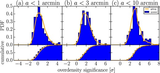
Histogram of overdensity significance of quasars (blue histograms) and g-dropouts (orange lines). Panels (a), (b), and (c) show histograms of the maximum overdensity significance centered on quasars and g-dropouts with radius (pMpc) 1΄(0.42), 3΄(1.25), and 10΄(4.2). On the vertical axis we show the probability distribution function (PDF) and the cumulative PDF. (Color online)
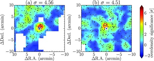
Two quasars found within 1΄ (0.42 pMpc) of a protocluster candidate. The quasars are indicated by the blue star symbols. The quasar in the center of each panel lies near a >4 σ maximum overdensity significance region of σ = 4.56 in panel (a) and 4.51 in panel (b). The color contours show the overdensity significance map, and the red circle shows the local maximum of the region. The black dots show the g-dropout galaxies, and the mask regions are indicated by the white regions. The size of each panel is 20΄ × 20΄. The quasar pair at z ≈ 3.6 from Onoue et al. (2018) is indicated in panel (b). (Color online)
Statistical tests of the correlation of the separations between quasars and protoclusters.*
Statistical tests of the correlation of the separations between quasars and protoclusters.*
We expect that the shape of the redshift distribution of quasars is not exactly the same as that of the g-dropout galaxies. Therefore, the correlations that we are looking for might be diluted by the slight differences in redshift of these samples; however, we confirmed that our results did not change even if we extracted 80 quasars at z = 3.5–4.0 or selected the quasars which satisfy the exact same selection criteria (1)–(5) as the g-dropouts. This result is robust even if extracting only for the overdense regions with >5 σ to enhance the purity of the sample: the p-value of the KS test between their distributions is 0.437; focused on the smaller scale < 0|${^{\circ}_{.}}$|2, the p-value is 0.67.
3.2 Stacked densities around quasars
To further investigate the average environment of quasars, we measured the median stacked overdensity significance map around all quasars and g-dropout galaxies (figure 5). Each galaxy overdensity significance map has a 1΄ spatial resolution estimated from the fixed apertures with a radius of 1|${^{\prime}_{.}}$|8. Here, to fairly compare their environments, we count only once those quasars that are also g-dropouts. Panels (a) and (b) show the overdensity significance map around quasars and g-dropouts, respectively. The g-dropout galaxies that were used to make these maps are the same as those used to define the overdensity significance.
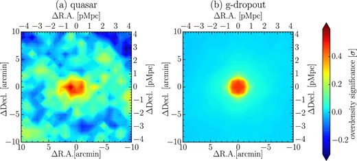
Median stacking overdensity significance map around quasars/g-dropouts. Panels (a) and (b) show the median stacking density map around quasars and g-dropouts, respectively. Their objects reside in the center of each panel. The size of each panel is 20΄ × 20΄. (Color online)
To more clearly show the difference, figure 6 shows the radial profile of the median stacked overdensity significance maps of figure 5. The blue (green) points show the median densities within a circular ring with a width of 1΄ in the case of quasars (g-dropouts). The error bars show the standard error of the mean. We find an interesting structure: the average density around quasars is slightly higher than that of g-dropout galaxies in the 1.0–2.5 pMpc-scale environment at the several sigma level, while for the smaller-scale environment, <0.5 pMpc, that of quasars is lower by about one sigma.

Radial profile of median stacked overdensity significance around quasars/g-dropouts. The blue points show the case of quasars. The bars indicate the 1 σ standard error. The median of radial distances of g-dropouts with 1 σ standard error bars are shown by green points. (Color online)
3.3 Rest-UV luminosities and black hole masses of quasars in overdense regions
We checked for differences between the luminosities of quasars inside and outside overdense regions. Figure 7 shows the relation between ambient overdense significances and the i-band absolute magnitudes of the quasars, which correspond to their rest-UV luminosity at this redshift. The absolute magnitudes are estimated from visual inspection of the redshift of each quasar in the SDSS DR12 catalog, Z_VI. Panels (a), (b), and (c) show the cases of the maximum overdensity significance within circles of radius 1΄, 3΄, and 10΄ centered on the quasars, respectively. In order to show whether our quasar sample is complete, we show the completeness limit (the gray shaded region), which corresponds to the BOSS limiting magnitude of r < 21.8, and assuming that r − i = 0.145, which is the median color of the SDSS quasar sample at z = 3.3–4.2. The Spearman rank correlation test shows correlation coefficients equal to 0.165, 0.153, and 0.199, and p-values equal to 0.0464, 0.0611, and 0.0146 for the three angular scales, respectively, suggesting weak correlations between quasar luminosity and environment with ∼2 σ significance. These results show that brighter quasars statistically tend to reside in lower density regions of g-dropout galaxies.
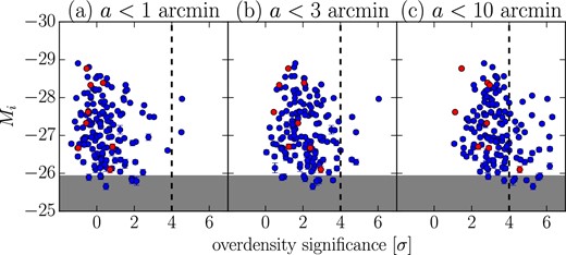
UV luminosities for overdensity significances about quasars. Panels (a), (b), and (c) show the relation between the i-band absolute magnitudes of quasars and the maximum overdensity significances centered on quasars with a radius of 1΄, 3΄, and 10΄, respectively. The FIRST-detected quasars are also shown with red points. The >4 σ overdense regions are to the right of the dashed line. The gray shaded region shows the complete limit, which corresponds to the BOSS limiting magnitude of r < 21.8. (Color online)
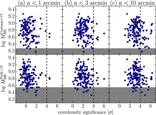
Black hole masses for overdensity significances about quasars using two black hole mass estimators: the Coatman et al. (2017) estimator (first line), and the Park et al. (2013) estimator (second line). Panels (a), (b), and (c) show the relation between the C iv-based back hole masses of quasars and the maximum overdensity significances centered on quasars with a radius of 1΄, 3΄, and 10΄, respectively. The FIRST-detected quasars are shown by red points. The >4 σ overdense regions are to the right of the dashed line. We show the complete limit (the gray shaded regions), which corresponds to the BOSS limiting magnitude of r < 21.8, assuming that the quasar spectrum energy density fν ∝ ν−0.5 and |$\Delta V_\mathrm{P}(\rm{C\,{\small {IV}}})=4385.06$| and |$V_\mathrm{C}^\mathrm{correct}(\rm{C\,{\small {IV}}})=2240.72\:$|km s−1, which are the median FWHM of the C iv line of the SDSS quasar sample at z = 3.3–4.2. (Color online)
Spearman rank correlation test results.
| UV luminosity | ρ* | p-value |
|---|---|---|
| Local peak within 1΄ | 0.165 | 0.0464 |
| Local peak within 3΄ | 0.153 | 0.0611 |
| Local peak within 10΄ | 0.199 | 0.0146 |
| C iv-based BH mass | ρ* | p-value |
| Coatman et al. (2017) | ||
| Local peak within 1΄ | −0.194 | 0.0273 |
| Local peak within 3΄ | −0.0969 | 0.263 |
| Local peak within 10΄ | −0.0985 | 0.257 |
| Park et al. (2013) | ||
| Local peak within 1΄ | −0.216 | 0.0136 |
| Local peak within 3΄ | −0.138 | 0.111 |
| Local peak within 10΄ | −0.140 | 0.107 |
*Spearman rank correlation test results for the relation between absolute i-band magnitudes (UV luminosity) and black hole masses of quasars and overdensity within a radius (pMpc) of 1΄ (0.42), 3΄ (1.25), and 10΄ (4.2). The correlation coefficient in the Spearman correlation test.
Finally, we also compare the black hole mass and environment for the FIRST-detected quasars. The fraction of the FIRST quasars tends to be high at the high black hole mass end, as can be seen in Ichikawa and Inayoshi (2017), and they do not lie in particularly overdense regions, although the sample is very small (the red points in figures 7 and 8).
4 Discussion
4.1 The low coincidence of quasars and protoclusters
We tried to find any positive correlations between quasars and protoclusters at z ∼ 4. Only two quasars were found to spatially coincide with protoclusters. However, for most quasars there is no correspondence with protoclusters. Here we will show how this result can be understood.
The total comoving cosmic volume covered by our survey (121 square degrees between z = 3.3 and z = 4.2) is about 1.18 cGpc3. The space density of our 151 quasars, which are almost completely observed (see figures 7 and 8), is thus about 3.74 × 10⁻⁷ h3 cMpc−3. The total number density of halos capable of hosting such quasars can be evaluated by correcting the quasar number density for duty cycle and viewing angle. The net lifetime of a quasar is believed to be about 106–108 yr from clustering or demographic analysis (e.g., Martini 2004). The cosmic time between z = 4.2 and z = 3.3 is ∼0.467 Gyr. So at any given time, we expect that about 0.2%–20% of the halos can host quasars. This increases the halo number density to 1.87 × 10⁻⁶–1.87 × 10⁻⁴ h3 cMpc−3. Next, we need to correct for viewing angle. We expect that at most 50%–70% percent of random viewing angles will be along our line of sight, producing our luminous quasars (Simpson 2005). Thus, the total number density of halos hosting quasar-like host galaxies is 2.67 × 10⁻⁶–3.74 × 10⁻⁴ h3 cMpc−3. On the other hand, the number density of local rich clusters of galaxies with >1014 M⊙ is about 1.26 × 10⁻⁵ h3 cMpc−3 (e.g., Rozo et al. 2009), which is consistent with the halo number density estimated by the halo mass functions from Behroozi, Wechsler, and Conroy (2013). The number density of halos capable of hosting quasars at z ∼ 4 is thus close to the number density of clusters today.
The halo mass of quasars is observationally estimated by clustering analysis as Mhalo ∼ 4–6 × 10¹² h−1 M⊙ at z > 3.5 (Shen et al. 2007), which is the minimum halo mass. About 30%–50% of these should evolve into halos with masses >1014 M⊙ at z = 0, based on the extended Press–Schechter (EPS) model (Press & Schechter 1974; Bower 1991; Bond et al. 1991; Lacey & Cole 1993). This estimate is likely to be a lower limit because the mean halo mass is about three times the minimum halo mass (e.g., Ishikawa et al. 2015). In principle, the number density and halo mass suggest that our quasars could be associated with protoclusters, assuming that the Shen et al. (2007) halo mass estimates are correct. However, our results also show that there is no association between the HSC-SSP Wide protoclusters and the majority of the quasars, since only 2 out of 151 quasars were found to reside near protoclusters.
Recently, Eftekharzadeh et al. (2015) derived a less massive quasar halo mass, Mhalo = 0.6 × 10¹² h−1 M⊙ at z ∼ 3, based on a larger sample by BOSS. He et al. (2018) showed that the average halo mass of z ∼ 4 less-luminous quasars, Mi ≳ −26, detected by HSC is ∼1 × 10¹² h−1 M⊙ . In GALFORM (e.g., Lacey et al. 2015), the halo mass function of quasars at z ∼ 4 is predicted to have a peak around Mhalo ∼ 0.3–1.0 × 10¹² h−1 M⊙ (Fanidakis et al. 2013; Orsi et al. 2016), which is about 10 times less massive than Shen et al. (2007), with a large range of mass distribution. Oogi et al. (2016) also predict a few × 1011 M⊙ for the median halo mass of quasars at z ∼ 4. It should be noted that the clustering strength of quasars is almost independent of their luminosity (e.g., Shen et al. 2013; Eftekharzadeh et al. 2015; He et al. 2018). The quasar halo mass of ∼0.3–1.0 × 10¹² h−1 M⊙ at z ∼ 4 provides a probability of only ∼1%–5% that the z = 0 descendant halo mass exceeds 1014 M⊙ . This seems to be reasonable for our results, suggesting that a typical quasar halo mass might be ≲ 1012 h−1 M⊙ at z ∼ 4.
If we were to adopt the high halo masses found by Shen et al. (2007), the lack of correspondence between the protoclusters and the quasars is even more striking. In this case, it is clear that our g-dropout protoclusters must trace the progenitors of much rarer, more massive clusters than the 1014 M⊙ halos assumed to be the typical descendants of the Shen et al. (2007) quasar hosts. For example, if the g-dropout protoclusters trace clusters only three times larger than 1014 M⊙ it would already lead to a 10 times lower number density due to the steep slope of the halo mass function at these high masses.
We can estimate the descendant halo masses at z ∼ 0 from the distribution of overdensity significances at the z ∼ 4 quasar positions (figure 3a) by using the light cone model (Henriques et al. 2012). We associate the overdensity significances which simulated g-dropout galaxies exist on with their z = 0 descendant halo masses by tracing back the halo merger tree from z = 0 to z ∼ 3.8. Figure 9 presents the distribution of overdensity significances of observed quasars at z ∼ 4 (blue histogram) and simulated g-dropout galaxies with the descendant halo masses of Mh, z = 0 = 1012 M⊙ –1013 M⊙ (orange line), Mh, z = 0 = 1013 M⊙ –1014 M⊙ (red line), and Mh, z = 0 > 1014 M⊙ (green line) in the simulation. We found that the predicted descendant halo mass distribution from the overdensity significances of our observed quasars at z ∼ 4 is roughly consistent with the mass distribution Mh, z = 0 = 1013 M⊙ –1014 M⊙ with p-value = 0.314, while inconsistent with those of Mh, z = 0 = 1012 M⊙ –1013 M⊙ and Mh, z = 0 > 1014 M⊙ with p-value = 0.00502 and 0.0332 in the KS test, respectively. Roughly speaking, luminous quasars at z ∼ 4 reside in the density environments which evolve into halos with a mass of ∼1013 M⊙ –1014 M⊙ .
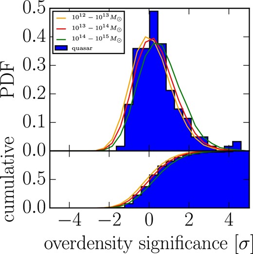
Correspondence between observational overdensity significances of quasars and their z = 0 descendant halo masses of quasars and simulated g-dropouts. The blue histogram shows the distribution of maximum overdensity significances centered on quasars with a radius of 1΄, which is exactly the same as figure 3a. The orange, red, and green lines indicate the simulated g-dropout overdensity significance distributions with z = 0 descendant halo masses Mh, z = 0 = 1012 M⊙ –1013 M⊙ , Mh, z = 0 = 1013 M⊙ –1014 M⊙ , and Mh, z = 0 > 1014 M⊙ , respectively. Their overdensity significances are those simulated for z ∼ 4. (Color online)
The finding that most quasars do not live in the >4 σ overdense regions is consistent with other results. At z < 2, many studies on quasar halo mass show that they reside in average halo masses (e.g., Coil et al. 2007), implying that they avoid the most overdense regions. This can be understood by the well-known environmental relation that passive, red early-type galaxies dominate in overdense regions (Dressler 1980; Baldry et al. 2004). The brightness of quasars is produced by strong black body radiation (big blue bump) from an optically thick accretion disk (e.g., Malkan & Sargent 1982). At higher redshift z ∼ 2–3, protocluster galaxies are on average found to be older and more massive than those in fields (Steidel et al. 2005; Koyama et al. 2013; Cooke et al. 2014). Thus, quasars may not necessarily appear in mature overdense regions because they may lack the wet mergers which lead to quasar activity (Lin et al. 2008).
The environment around a quasar may not appear as an overdense region due to the strong radiation from the quasar (quasar-mode AGN feedback: Kashikawa et al. 2007). This will be discussed in more detail in the next subsection.
We can compare our results with Adams et al. (2015), who found one overdense region of LBGs (r < 25.0) in a sample of nine luminous SDSS quasars, Mi < −28.0, at z ∼ 4. If we choose from our 151 quasars a sample with the same luminosity range as that of their 9 quasars, we find that only 1 out of 27 quasars resides in a protocluster. Although the fraction of quasars in overdensities appears to be three times higher in Adams et al. (2015), we note that none of their quasars lie in overdensities as significant as the >4 σ overdensities that we selected in our work. Also, it is interesting to note that the evidence for a physical overdensity in the case of the quasars in Adams et al. (2015) only appeared after spectroscopic follow-up, showing that spectroscopic redshifts are crucial to obtaining definite answers.
We also found that no FIRST-detected quasars reside in >4 σ overdense regions. On the other hand, Hatch et al. (2014) showed at high statistical significance that radio-loud AGNs reside in denser Mpc-scale environments than similarly massive radio-quiet galaxies at z = 1.3–3.2. Venemans et al. (2007) found that six out of eight radio galaxies reside in overdense regions. This difference from our result might be due not only to the above reasons, but also the difference in selection criteria. The radio-loud AGNs from Hatch et al. (2014) and Venemans et al. (2007) are about ten times more luminous in the radio than our FIRST-detected quasars, and the environments where they are measured are entirely different. It is therefore difficult to assess at this point whether our results are consistent or not. We are also limited by the small sample size of only eight quasars. In the future, we will investigate in detail the environments of large numbers of radio-loud and radio-quiet quasars using the full 1400 deg2 of the HSC-SSP Wide survey.
4.2 The relation between density and quasar properties
We found that UV-brighter quasars statistically tend to reside in less dense regions of g-dropout galaxies. In addition, the quasars with the most massive black holes tend to avoid overdense regions. Figure 10 shows the distributions of overdensity significances of bright quasars, which are defined by being brighter than the median of the absolute i-band magnitudes of the quasar sample. In fact, the brighter quasars significantly reside in less dense regions than g-dropout galaxies, at least in the 1΄-scale environment. The results are summarized in table 4. Earlier work has suggested that the strong radiation from quasars may provide negative feedback and suppress nearby galaxy formation, especially for low-mass galaxies (Kashikawa et al. 2007). We use the near-zone sizes (e.g., Fan et al. 2006; Mortlock et al. 2011) of our quasar sample to evaluate the scale of AGN feedback. We estimate the intrinsic flux by fitting a single power law to the continuum free of line emission at ∼1340–1360 Å, 1440–1450 Å, and 1700–1730 Å. The IGM transmission curves are calculated by the observed fluxes divided by the intrinsic fluxes blueward of Lyα, and then fitted by a single power law. Then, the near-zone size is defined by the proper radius at which the fitted transmission first falls below 10% (Fan et al. 2006; Mortlock et al. 2011). Figure 11 shows the relation between the overdensity significance and near-zone size for each quasar. Although the scatter is large, it appears that quasars tend to have much smaller near-zones when their overdensity significance is larger than ∼2σ. On the other hand, quasars in lower density regions can have the full range of near-zone sizes. The statistical coefficient ρ and the p-value are −0.232 and 0.00798 in the Spearman rank correlation test. These findings may indicate that perhaps galaxy formation is delayed in overdense regions due to the quasar feedback. Another possibility is that the near-zones in overdense regions are smaller due to the much higher gas densities that are more difficult to fully ionize.
Histogram of overdensity significance of bright quasars. Panels (a), (b), and (c) show the histograms of the maximum overdensity significance centered on quasars with a radius (pMpc) of 1΄ (0.42), 3΄ (1.25), and 10΄ (4.2), respectively. (Color online)
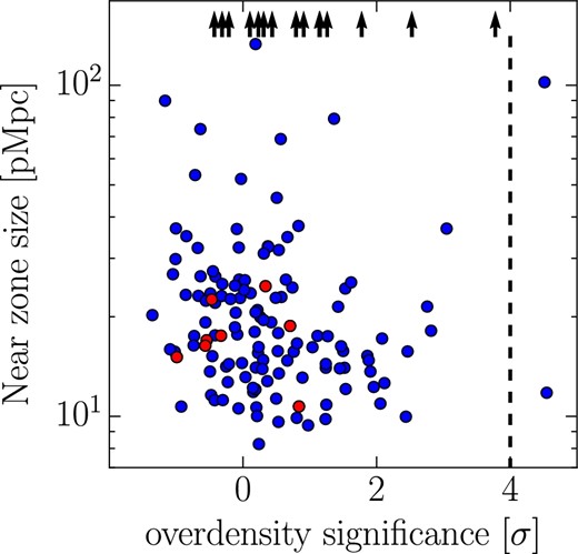
Near-zone size of quasars as a function of the overdensity significance. The red points show the FIRST-detected quasars. The black arrows show quasars with near-zone sizes larger than 150 pMpc. The >4 σ overdense regions are to the right of the dashed line. (Color online)
Statistical test for correlation of position between bright quasars and protoclusters.
| KS p-value | Median quasar | Median g-dropout | |
|---|---|---|---|
| Local peak within 1΄ | 0.0392 | 0.189 | 0.474 |
| Local peak within 3΄ | 0.702 | 1.78 | 1.94 |
| Local peak within 10΄ | 0.849 | 3.06 | 3.12 |
| KS p-value | Median quasar | Median g-dropout | |
|---|---|---|---|
| Local peak within 1΄ | 0.0392 | 0.189 | 0.474 |
| Local peak within 3΄ | 0.702 | 1.78 | 1.94 |
| Local peak within 10΄ | 0.849 | 3.06 | 3.12 |
Considering the viewing angle of type-1 quasars, this effect should be the most significant on the number density of galaxies along the quasar lines of sight (LOS), and become weaker as it goes away from the LOS. The tendency towards low density at <1΄ as seen in figures 6 and 10 could also be caused by the effect. Our statistical test to see the possible UV luminosity, black hole mass, and near-zone size dependence on the distance to the nearest overdense region (see figures 7, 8, and 11) agrees with the hypothesis, although projection effects may smear out this small-scale over-(under-)density signal.
5 Conclusions
We have used a statistically significant sample of 179 protoclusters from the HSC survey (Toshikawa et al. 2018) to investigate the spatial correlation between the protoclusters and quasars at z ∼ 4. Note that this sample is around 10 times as large as the number of all previously known protoclusters. We found 151 SDSS quasars at z = 3.3–4.2 in effective areas of the HSC-Wide layer, whose redshift range corresponds to the g-dropout selection function.
We showed, for the first time, that quasars statistically do not reside in the most massive halos at z ∼ 4, assuming that environment correlates with halo mass. We used stacking analysis to find that the average density of g-dropout galaxies around quasars is slightly higher than that around g-dropout galaxies on 1.0–2.5 pMpc scales, while at <0.5 pMpc that around quasars tends to be lower. We also find that quasars with higher UV luminosity or with more massive black holes tend to avoid the most overdense regions, and that the quasar near-zone sizes are anti-correlated with overdensity.
We discussed some possibilities for why the most luminous quasars do not live in the most overdense regions: (1) wet mergers do not often occur in mature overdense regions, (2) quasar-mode AGN feedback disturbs galaxy formation, and (3) quasar halo mass at z ∼ 4 is not massive enough to evolve into cluster halo mass.
In the future, we will investigate a possible correlation between AGNs and >1000 complete protocluster candidates found in the HSC-SSP final data release with better statistical accuracy.
Acknowledgements
This work is based on data collected at the Subaru Telescope and retrieved from the HSC data archive system, which is operated by the Subaru Telescope and Astronomy Data Center at the National Astronomical Observatory of Japan.
Alvaro Orsi provided constructive comments and warm encouragement about AGN modeling in the semi-analytic model. Jim Bosch, Hisanori Furusawa, Robert H. Lupton, Sogo Mineo, and Naoki Yasuda provided helpful comments and discussions on the treatment of the HSC data. NK acknowledges support from JSPS grant 15H03645. This work was partially supported by the Overseas Travel Fund for Students (2016) of the Department of Astronomical Science, SOKENDAI (the Graduate University for Advanced Studies). MT is supported by JSPS KAKENHI Grant Number JP15K17617. Authors RO and YTL received support from CNPq (400738/2014-7).
The Hyper Suprime-Cam (HSC) collaboration includes the astronomical communities of Japan and Taiwan, and Princeton University. The HSC instrumentation and software were developed by the National Astronomical Observatory of Japan (NAOJ), the Kavli Institute for the Physics and Mathematics of the Universe (Kavli IPMU), the University of Tokyo, the High Energy Accelerator Research Organization (KEK), the Academia Sinica Institute for Astronomy and Astrophysics in Taiwan (ASIAA), and Princeton University. Funding was contributed by the FIRST program from the Japanese Cabinet Office, the Ministry of Education, Culture, Sports, Science and Technology (MEXT), the Japan Society for the Promotion of Science (JSPS), the Japan Science and Technology Agency (JST), the Toray Science Foundation, NAOJ, Kavli IPMU, KEK, ASIAA, and Princeton University.
This paper makes use of software developed for the Large Synoptic Survey Telescope. We thank the LSST Project for making their code available as free software at http://dm.lsst.org.
The Pan-STARRS1 Surveys (PS1) have been made possible through contributions of the Institute for Astronomy, the University of Hawaii, the Pan-STARRS Project Office, the Max-Planck Society and its participating institutes, the Max Planck Institute for Astronomy, Heidelberg and the Max Planck Institute for Extraterrestrial Physics, Garching, The Johns Hopkins University, Durham University, the University of Edinburgh, Queen’s University Belfast, the Harvard-Smithsonian Center for Astrophysics, the Las Cumbres Observatory Global Telescope Network Incorporated, the National Central University of Taiwan, the Space Telescope Science Institute, the National Aeronautics and Space Administration under Grant No. NNX08AR22G issued through the Planetary Science Division of the NASA Science Mission Directorate, the National Science Foundation under Grant No. AST-1238877, the University of Maryland, Eotvos Lorand University (ELTE), and the Los Alamos National Laboratory.
References
