


Abstract
We investigate the galaxy overdensity around proto-cluster scale quasar pairs at high (z > 3) and low (z ∼ 1) redshift based on the unprecedentedly wide and deep optical survey of the Hyper Suprime-Cam Subaru Strategic Program (HSC-SSP). Using the first-year survey data covering effectively ∼121 deg2 with the 5σ depth of i ∼ 26.4 and the SDSS DR12Q catalog, we find two luminous pairs at z ∼ 3.3 and 3.6 which reside in >5σ overdensity regions of g-dropout galaxies at i < 25. The projected separations of the two pairs are R⊥ = 1.75 and 1.04 proper Mpc (pMpc), and their velocity offsets are ΔV = 692 and 1448 km s−1, respectively. This result is in clear contrast to the average z ∼ 4 quasar environments as discussed in Uchiyama et al. (2018, PASJ 70, S32) and implies that the quasar activities of the pair members are triggered via major mergers in proto-clusters, unlike the vast majority of isolated quasars in general fields that may turn on via non-merger events such as bar and disk instabilities. At z ∼ 1, we find 37 pairs with R⊥ < 2 pMpc and ΔV < 2300 km s−1 in the current HSC-Wide coverage, including four from Hennawi et al. (2006, AJ, 131, 1). The distribution of the peak overdensity significance within two arcminutes around the pairs has a long tail toward high-density (>4σ) regions. Thanks to the large sample size, we find statistical evidence that this excess is unique to the pair environments when compared to single-quasar and randomly selected galaxy environments at the same redshift range. Moreover, there are nine small-scale (R⊥ < 1 pMpc) pairs, two of which are found to reside in cluster fields. Our results demonstrate that <2 pMpc scale quasar pairs at both redshift ranges tend to occur in massive haloes, although perhaps not the most massive ones, and that they are useful in searching for rare density peaks.
1 Introduction
The subject of how active galactic nuclei (AGN) connect to their surrounding galaxy formation and host dark matter haloes has been a matter of debate in modern extragalactic astronomy. When one assumes that supermassive black holes (SMBHs) grow primarily via gas accretion, the triggering mechanism of luminous quasars would be major mergers of gas-rich galaxies, which transform plenty of cold gas into the central SMBHs (e.g., Hopkins et al. 2008; Alexander & Hickox 2012). The MBH–σ* relation (e.g., Magorrian et al. 1998; Kormendy & Ho 2013) suggests a co-evolutionary growth history of SMBHs and host galaxies throughout the cosmic epoch in which massive galaxies host large SMBHs.
To investigate how the most mature clusters in the local universe are formed along with the hierarchal large-scale structure formation, AGN have been used for proto-cluster searches at high redshift. This is motivated by the assumption that galaxies in high-density regions have earlier episodes of star formation and SMBH growth than those in normal and poor environments. Since gas-rich major mergers would happen more frequently in massive haloes than in less-massive ones, luminous AGN can be used as landmarks of proto-clusters, while the blind searches of such rare density peaks requires a wide-field observation. There are various studies testing the validity of using AGN for proto-cluster searches. For example, Venemans et al. (2007) clearly show that radio galaxies are likely to be associated with proto-clusters at z > 2 based on their Lyman α emitter (LAE) searches. Wylezalek et al. (2013) show that radio-loud AGN prefer massive environments using sources selected by the Infrared Array Camera (Fazio et al. 2004) of the Spitzer Space Telescope, suggesting that high-density environments induce high spins of the SMBHs and enhancement of the AGN radio jets. On the other hand, environment studies of the highest-redshift quasars show that luminous z > 6 quasars are not necessarily associated with rich environments (Mazzucchelli et al. 2017, and reference therein). Moreover, a deep and large spectroscopic sample of 2 < z < 3 quasars from the Baryon Oscillation Spectroscopic Survey (BOSS: Dawson et al. 2013) implies that the redshift evolution of the quasar auto-correlation signal gets flattened from lower redshift (Eftekharzardeh et al. 2015). Although their result is inconsistent with a z > 3 study carried out by Shen et al. (2007) and the reason is unclear, it may imply that highly energetic feedback from quiescent AGN suppresses further cold-gas assembly on to the SMBHs in the most massive haloes (“radio-mode” feedback). Thereby, these arguments follow that the host halo of a luminous quasar at high redshift is not the most massive. This scenario is supported by several semi-analytical studies (e.g., Fanidakis et al. 2013; Orsi et al. 2015).
The Hyper Suprime-Cam (HSC: Miyazaki et al. 2012) is a new optical camera installed at the prime focus of the Subaru telescope. With the 8.2 m mirror of the Subaru, ten minutes’ imaging goes as deep as rlim,5σ ∼ 26, which is three magnitudes deeper than the Sloan Digital Sky Survey (SDSS: York et al. 2000). The most characteristic feature of the HSC is its gigantic field-of-view of 1.5 degree diameter. Taking advantage of the survey efficiency of the camera, the HSC Subaru Strategic Program (HSC-SSP) covers 1400 deg2 with its five broad-band filters in the Wide layer.1 This survey is a five-year survey, which began in 2014 March. Its first ∼100 deg2 data of the Wide, Deep, and UltraDeep layers has been open to the public since 2017 February (Aihara et al. 2018b). Since the survey started its enormously wide field observation, Toshikawa et al. (2018) found 179 promising proto-cluster candidates at z ∼ 3.8 over 121 deg2 currently available among the collaboration. This number overwhelms that of the previously known proto-clusters at the same redshift range, enabling them to investigate the clustering of proto-clusters for the first time. Their g-dropout catalog, which efficiently selects Lyman break galaxies, is used for a quasar environment study by Uchiyama et al. (2018), which is our companion paper. In this paper, they exploit the catalog to examine how well quasars at 3.3 < z < 4.2 trace the HSC proto-clusters based on their 151 BOSS quasar sample, finding that the luminous quasars in general do not reside in rich environments when compared to g-dropout galaxies. In particular, there are only six cases that the individual luminous quasars are hosted in the HSC proto-clusters within three arcminutes (∼1.3 proper Mpc, hereafter pMpc) from the density peaks. Their result sheds a new light on the triggering mechanism of luminous quasars from an environmental point of view; the quasar activity at high redshift is more common in general environments than previously thought. One interpretation would be that the major merger is not the only mechanism to trigger a luminous quasar and that other channels, such as the secular process (bar and disk instabilities), which closes in its own system and has less to do with its environment, play a significant role. In fact, recent studies have shown that the morphology of luminous-quasar hosts at z < 2 are not highly distorted and are not significantly different from that of inactive galaxies (e.g., Mechtley et al. 2016; Villforth et al. 2017). Another way to explain their result is the strong AGN feedback, which suppresses star formation in the vicinity of quasars. It is also possible that the majority of star-forming galaxies around z ∼ 4 quasars are dusty and thus highly obscured, for which optical-based selection completeness is low.
When one assumes that major mergers dominate the role of triggering quasars in massive haloes, it is likely that environments around multiple quasars, i.e., a physical association of more than one quasar in close separation are more biased, and they are much more efficient in pinpointing proto-clusters. While such a population is extremely rare, there are several studies of pair and multiple quasars. Djorgovski et al. (1987) first report the discovery of a binary quasar at z = 1.345, a radio source PKS 1145−071, separated by 4|${^{\prime\prime}_{.}}$|2. A small number of z > 4 quasar pairs with less than 1 pMpc projected separation has been reported (Schneider et al. 2000; Djorgovski et al. 2003; McGreer et al. 2016). Based on the SDSS, Hennawi et al. (2006, 2010) construct large catalogs of spectroscopically confirmed quasar pairs at z < 3 and 3 < z < 4, respectively. Quasar pairs with sub-pMpc-scale separation are of particular interest for the study of the small-scale clustering of quasars. Several papers argue that quasar clustering is enhanced on such a small scale, which is suggestive of enhanced quasar activity in rich environments (e.g., Hennawi et al. 2006; Eftekharzadeh et al. 2017, but also see Kayo & Oguri 2012). Regarding the environments, most of the previous works focus on z < 1 pairs with ∼10 sample sizes (e.g., Boris et al. 2007; Farina et al. 2011; Green et al. 2011; Sandrinelli et al. 2014). While the observation depth and the target selection are different among these studies, they all suggest that the extremely rare quasar pairs are not always associated with significant overdensity of galaxies. At high redshift, Fukugita et al. (2004) look for the overdensity enhancement around a z = 4.25 quasar pair, SDSS J1439−0034, but see no significant difference from a general field within a 5.8 arcmin2 area. On the other hand, it is remarkable that Hennawi et al. (2015) show an exceptionally strong enhancement of the LAE surface density around a z = 2 quasar quartet (“Jackpot nebulae”) especially at <100 pkpc scale, demonstrating the extremeness of multiple quasar environments. Moreover, Cai et al. (2017) find an extremely massive overdensity of LAEs at z = 2.32 which is associated with multiple quasars.
This paper focuses on the galaxy overdensity around pairs of BOSS quasars up to z ∼ 3.6, thanks to the unprecedented coverage and depth of the HSC-SSP data set. The outline of this paper is as follows. In section 2, we describe our quasar-pair sample at high redshift (3.3 < z < 4.2) and introduce how we select surrounding galaxies using the HSC-SSP photometric data set. In section 3, we show that two quasar pairs at z ∼ 3.3 and ∼3.6 are both associated with the HSC proto-clusters, supporting that the rare occurrence of <2 pMpc-scale pairs traces rich environments. Section 4 describes our overdensity measurements around 37 quasar pairs at z < 1.5, including four pairs from literature, using the photometric redshift catalog of the HSC-SSP. We find statistical evidence that a significantly higher fraction of quasar pairs reside in dense environments than single quasars and randomly selected galaxies, which is described in section 5. We discuss the quasar-pair environments in section 6, especially comparing them with the study of single-quasar environments at z ∼ 3.8 (Uchiyama et al. 2018). Finally, the summary is given in section 7.
Throughout this paper, we adopt a ΛCDM cosmology with H0 = 70 km s−1 Mpc−1, Ωm = 0.3, and |$\Omega _\Lambda =0.7$|. Unless otherwise stated, the magnitudes cited in this paper are the CModel magnitude (in AB system), which is derived by fitting images with a combination of the exponential and de Vaucouleurs profiles. The CModel magnitude is conceptionally the same as the Point Spread Function (PSF) magnitude for point sources.
2 Data and sample selection
2.1 Effective region in the HSC-Wide data set
In this paper, we use a photometric catalog of the HSC-SSP Wide survey for our surrounding galaxy selection. The photometric catalog using a dedicated pipeline (hscPipe: Bosch et al. 2018) has been opened to the collaboration, the latest data set of which is denoted as “DR S16A”, with its Wide component covering ∼170 deg2 in five broad-band filters (grizy). This area consists of several large fields along the equator (W-GAMA09H, W-Wide12H, W-GAMA15H, W-VVDS, W-XMMLSS) and one field at Dec = 43° (W-HECTMAP). The average 5σ-limiting magnitudes are as follows: g ∼ 26.8, r ∼ 26.4, i ∼ 26.4, z ∼ 25.5, and y ∼ 24.7.2 We share the g-dropout catalog of the HSC proto-cluster search project (Toshikawa et al. 2018). To take into account the partly inhomogeneous imaging in each HSC filter over the large survey regions, Toshikawa et al. carefully remove any areas with shallow depths in either g, r, or i bands based on sky noise measurements at each 12 × 12 arcmin2 sub-region (“patch” in the HSC-SSP terminology), as well as the masked regions, for example, around saturated stars, at the edge of the images, and on bad pixels based on the photometry flags of the hscPipe (see section 2 of Toshikawa et al. 2018 for more details). As a result, they construct a highly clean and uniform g-dropout galaxy sample over a total effective area of ∼121 deg2. Specifically, the W-GAMA09H field is discarded in our analysis, because the number counts of the g-dropout galaxies has an offset compared to the other fields in the bright magnitude range due to its shallow depth in the r band.
2.2 Quasar pair sample at 3 < z < 4
In this section, we present our selection and sample of quasar pairs at 3 < z < 4. We use the latest catalog of spectroscopically confirmed quasars from the SDSS-iii BOSS survey (DR12Q: Pâris et al. 2017), which contains about 300000 quasars in 9376 deg2 down to g = 22.0 or r = 21.85. While the BOSS survey originally targets quasars at 2.15 ≤ z ≤ 3.5, the redshift distribution of the DR12Q sample has a wide skirt up to z ∼ 6.4. Moreover, the DR12Q catalog has a secondary redshift peak at z ∼ 0.8, which is due to the SDSS-color similarity of quasars at this redshift range to that of 2 < z < 3 quasars, enabling us to also investigate low-redshift quasar environments as described in section 4. We require secure redshift determination using flags given in the DR12Q catalog (i.e., ZWARNING=0).
Since we assume a situation where more than one quasar emerges in the same massive halo, we define quasar pairs as two quasars with their separation being less than the size of massive proto-clusters. We extract quasar pairs from the DR12Q catalog following a framework given by a simulation done by Chiang, Overzier, and Gebhardt (2013). According to their definition of the most massive proto-clusters, which are the progenitors of Mhalo,z = 0 > 1015M⊙ clusters, and their characteristic size at the concerned redshift, we extract quasar pairs with their projected proper distance of R⊥ < 4 pMpc and velocity offset of ΔV < 3000 km s−1. This definition is more relaxed than previous studies such as Hennawi et al. (2010), since they assume that the pairs are gravitationally bound systems with R⊥ < 1 pMpc. The redshift range is limited to 3.3 < z < 4.2 where the selection completeness of the HSC g-dropouts is over 0.4 (Ono et al. 2018). The Lyman break of galaxies at this range is shifted to the r band, and therefore g − r and r − i colors can be used to distinguish those galaxies from contaminants such as main-sequence stars and z < 1 galaxies. The velocity offset between the quasar members in a pair ΔV is determined from the SDSS’s visually inspected redshifts (Z_VI). Considering the uncertainty of the BOSS redshifts primarily relying on the Lyman break and LAE (∼1000 km s−1), possible peculiar motion between the pair members (∼500 km s−1), and also their physical separation in the radial direction, we apply ΔVmax = 3000 km s−1 as the maximum velocity offset of the z ∼ 3.8 pairs. Finally, the BOSS quasar spectra are visually checked to confirm their secure classification and redshift determination.
As a result, two pairs of quasars are found at z ∼ 3.6 and z ∼ 3.3 from the DR12Q catalog. Table 1 lists the two pairs with their angular separation Δθ, projected separation R⊥, and velocity offset ΔV, in which the average redshift of the two quasars in pairs is regarded as the pair redshift. QSOP1 is a pair of quasars at z = 3.585 and z = 3.574 with an angular separation of Δθ = 241″ (R⊥ = 1.75 pMpc) and velocity offset of ΔV = 692 km s−1. QSOP2 is a quasar pair at z = 3.330 and z = 3.309, which is close to the edge of our redshift cut, with an angular separation of Δθ = 139″ (R⊥ = 1.04 pMpc) and velocity offset of ΔV = 692 km s−1. Note that only Fukugita et al. (2004) has investigated the overdensity around z > 3 quasar pairs before this study. We search for their radio counterparts in the Faint Images of the Radio Sky at Twenty cm survey (FIRST; 14Dec17 version: Becker et al. 1995) within 30″ radius, but find that none of them are detected. There are ∼30 pairs in the whole HSC-Wide coverage (i.e., 1400 deg2). The complete analysis of these pair environments will be done after the HSC-SSP survey is completed. Note that our pair selection is incomplete for small-scale pairs due to the fiber collision limit of the BOSS survey (Δθ = 62″). We check whether high-redshift physical pairs previously identified in literature (i.e., Schneider et al. 2000; Hennawi et al. 2010) are covered in DR S16A, but do not find any suitable pairs in our redshift range. There are several already-known pairs in the entire HSC-SSP survey regions, as we describe in subsection 6.1.
Quasar pair sample at 3 < z < 4.
| ID* | RA† | Dec† | Redshift‡ | i § | Δθ‖ | R ⊥ ♯ | ΔV** |
|---|---|---|---|---|---|---|---|
| (J2000.0) | (J2000.0) | [mag] | [″] | [pMpc] | [km s−1] | ||
| QSOP1 | 22h14m52|${^{\rm s}_{.}}$|49 | +01°11΄19|${^{\prime\prime}_{.}}$|9 | 3.585 | 21.167 ± 0.002 | 240.6 | 1.75 | 692 |
| 22h14m58|${^{\rm s}_{.}}$|38 | +01°07΄36|${^{\prime\prime}_{.}}$|1 | 3.574 | 20.380 ± 0.001 | ||||
| QSOP2 | 16h14m47|${^{\rm s}_{.}}$|39 | +42°35΄25|${^{\prime\prime}_{.}}$|2 | 3.330 | 20.373 ± 0.001 | 139.0 | 1.04 | 1448 |
| 16h14m51|${^{\rm s}_{.}}$|35 | +42°37΄37|${^{\prime\prime}_{.}}$|2 | 3.309 | 20.092 ± 0.001 |
*Pair ID.
†HSC coordinates.
‡SDSS DR12Q visual redshift (Z_VI).
§Extinction-corrected HSC-i magnitude.
‖Angular separation in arcseconds.
♯Projected separation in physical scale.
**Velocity offset of the pairs in km s−1.
2.3 Imaging data and method
The g-dropout selection in this paper is the same as Toshikawa et al. (2018). We first apply a magnitude cut of i < 25 (= ilim, 5σ − 1.4) to measure the overdensity in a magnitude range satisfying high completeness. Since this threshold corresponds to ∼M* + 2 at z ∼ 4 (Bouwens et al. 2007), where M* denotes the characteristic magnitude, our density measurements are limited to the bright population. In addition, we require significant detection in the r (<rlim, 3σ) and i (<ilim, 5σ) bands to remove contaminants such as artificial and moving objects. It is noted that the broad-band selection of Lyman break galaxies has a large uncertainty in redshift, corresponding to ∼200 pMpc in the line-of-sight direction, which is much larger than the projection direction. Then, the following color cuts are applied.
Our overdensity measurements of g-dropout galaxies in the quasar-pair fields are as follows. First, we extract g-dropout galaxies within a 2 × 2 deg2 field centered on the pair in the projection plane. Then, we set a square grid on the field at 0.6΄ intervals to measure the number count of g-dropouts at each position within a 1.8΄ aperture, corresponding to the size of a typical proto-cluster at z ∼ 4 (0.75 pMpc). We calculate the average and standard deviation of the g-dropout counts over the effective region (see subsection 2.1) inside the 2 × 2 deg2 fields. Blank grids where no galaxies exist inside the aperture are also masked out. The total area effectively used in 2 × 2 deg2 is 2.44 deg2 for QSOP1 and 2.19 deg2 for QSOP2, which are large enough to calculate the field number counts. After deriving the significance map over the wide area, we zoom-in on the pair vicinity of 12 × 12 arcmin2 (∼5 × 5 pMpc2) to see its local overdensity significance. The arbitrary zoom-in scale is chosen to be larger than the pair separation and thus enough to see the overdensity structure in the quasar-pair fields.
3 Result I: z > 3 quasar-pair environments
3.1 Discovery of proto-clusters at z = 3.3 and 3.6
This section shows the result of the overdensity measurements for the two quasar-pair fields at z > 3. We find significant overdensity in both pair fields, with peak significance σpeak = 5.22σ and 5.01σ, which is summarized in table 2. Figure 1 shows the overdensity profile of the pair fields where the color contours indicate the g-dropout overdensity significance based on the g-dropout counts. The pair members are shown by stars and g-dropout galaxies are shown by circles. The QSOP1 field shows a filament-like structure in the westward direction and the QSOP2 field shows a core-like structure with several smaller density peaks in the vicinity. The four quasars themselves are not selected in our dropout selection due to their relatively blue g − r colors (0.3 ≤ g − r ≤ 0.9), which could be explained by the intrinsic power-law shape of the quasar continuum declining toward longer wavelength. The cumulative number counts of the g-dropouts within five arcminutes from the pair centers are shown in figure 2 with open symbols, compared with those of the 2 × 2 deg2 general fields used for the density measurements.4 Overall, the number counts are about more than twice higher in all (non-zero) magnitude bins, even within such a large projected area corresponding to ∼2 pMpc radius. Specifically, there are two bright dropouts at 21.2 < i < 21.4 in the QSOP1 field, which is six times higher density than the general fields. Although the redshift uncertainty in our dropout selection is large, our result strongly suggests that these pairs are associated with massive environments, namely proto-clusters.
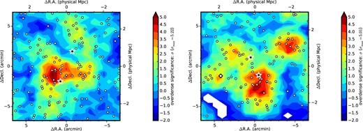
Overdensity profile of g-dropout galaxies (12 × 12 arcmin2) around QSOP1 (left) and QSOP2 (right). The quasar pairs are shown by black stars. The surrounding g-dropouts are shown by white circles. The g-dropout overdensity significance is shown by color contours. The region where no galaxies are found is masked. A white diamond in the QSOP2 field shows the quasar candidate, HSC J161506+423519 (i = 22.30). The physical scale from the pair center is also indicated. (Color online.)
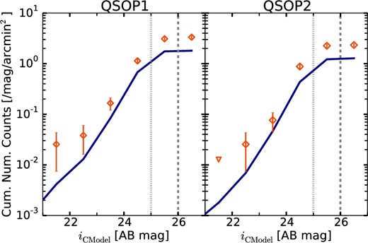
Cumulative i-band number counts of the g-dropouts within five arcminutes from the pair centers (left: QSOP1; right: QSOP2). In each panel, the open symbols show those of the pair field with Poisson error bars. Magnitude bins with zero source count are shown by upside-down triangles. The solid line shows the number counts of the field where the pair vicinity is excluded. The i = 25 and i = 26 magnitude thresholds are shown by vertical dotted and dashed lines, respectively. (Color online.)
Overdensity significance around two z > 3 quasar pairs based on i < 25 g-dropouts.
| ID | σpeak* | σQ1† | σQ2† | (Nave ± σSTD)‡ |
|---|---|---|---|---|
| QSOP1 | 5.22 | −0.02 | 3.30 | 5.80 ± 2.91 |
| QSOP2 | 5.01 | 4.21 | 2.23 | 4.40 ± 2.52 |
| ID | σpeak* | σQ1† | σQ2† | (Nave ± σSTD)‡ |
|---|---|---|---|---|
| QSOP1 | 5.22 | −0.02 | 3.30 | 5.80 ± 2.91 |
| QSOP2 | 5.01 | 4.21 | 2.23 | 4.40 ± 2.52 |
*Overdensity significance.
†Significance above each quasar. The former and latter quasars in table 1 are denoted as Q1 and Q2, respectively.
‡Average number and standard deviation (=σSTD) of g-dropouts within a 1|${^{\prime}_{.}}$|8 radius aperture.
Indeed, QSOP1 and QSOP2 fields are part of the HSC proto-clusters cataloged in Toshikawa et al. (2018). The two fields also have high sigma peaks, over 4σ, in their measurements (4.8σ and 4.0σ), which are likely to evolve in massive clusters in the local universe with a descendant halo mass Mhalo, z = 0 > 1014 M⊙. It is notable that these two fields are not the richest among the HSC proto-clusters, which could suggest that even quasar pairs do not trace the most massive haloes. The reason why the significance in our measurements is slightly higher than their measurements is the difference of the area used for the significance measurements. In Toshikawa et al. (2018), they measure the average and standard deviation of g-dropout counts over the whole S16A HSC-Wide area, deriving the average Nave, Wide = 6.39 ± 3.24. In our study, we measure the same quantities in an area approximately corresponding to the HSC field-of-view around the pairs. Therefore, Toshikawa et al.’s overdensity measurements reflect not only the intrinsic galaxy density distribution but also a different completeness over the large area due to the different observation depth taken in various seeing conditions and the different times being covered while dithering. Indeed, the peak significance of the two pair fields is smaller in our measurements, and both fields, especially QSOP2 at the edge of the W-HECTMAP, have smaller Nave than the measurements of Toshikawa et al. (2018).
For the two proto-clusters, we find that local peaks are close to one of the pair members, but not to the other one (see table 1). For QSOP1, the significance just above the two quasars are not high and, in particular, HSC J221452+011119 (the upper one in figure 1) is at the outskirts of the overdensity profile. This is also the case for QSOP2, as HSC J161451+423737 (the upper one) is at the gap of the density peaks. Nevertheless, there are only six out of 151 quasars in Uchiyama et al. (2018) measurements with which >4σ overdensity regions are associated within three arcminutes from the HSC proto-clusters, and intriguingly three of them are the quasar pairs: the two QSOP1 quasars and one QSOP2 quasar (HSC J161447+423525). Therefore, our result may indicate that pairs of quasars are likely related to rich environments, but they do not emerge at the central peak of galaxy density.
To investigate the overdensity structure further, the overdensity profiles of the same two fields are measured again including fainter g-dropouts down to the approximate 5σ limiting magnitude. Figure 3 shows the local significance maps of g-dropouts down to i < 26 (∼ilim, 5σ), for which only the i-band magnitude cut is loosened by one magnitude in the original dropout selection criteria. The circles and stars are the same as in figure 1, and the black dots show the g-dropouts with 25 ≤ i < 26. In the two significance maps, the overdensity structures become more extended and centered around the pairs in figure 3. While the completeness falls down from i > 25 as is also indicated in figure 2, the profiles would trace real structures assuming that the completeness is independent of local positions. Therefore, we conclude that these proto-clusters have filament-like extended structures and likely host the luminous quasars pairs members inside. We discuss the interpretation of our results in subsection 6.1, comparing single-quasar environments.
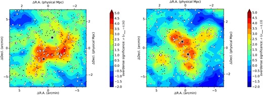
Same significance maps for QSOP1 and QSOP2, but with fainter g-dropouts down to i = 26.0. The black dots show the faint (25 ≤ i < 26) dropouts. The overdensity significance are measured with all i < 26.0 dropouts. (Color online)
3.2 A faint quasar candidate in the pair fields
We inspect the possibility that the two proto-clusters we find host other quasars fainter than the BOSS depth limit. Here, we assume a pure point-source morphology and search for faint quasar candidates among the g-dropouts in the two pair fields. For this purpose, a shape parameter included in the HSC-SSP data set is used, which gives a rough shape measurement based on the second moment of the object image. We take the i-band shape parameter, since the i-band observation in the HSC-SSP is executed in good seeing conditions (typically 0|${^{\prime\prime}_{.}}$|56). Using the ratio of the g-dropout moment (ishape_sdss, Iij) over the PSF moment (ishape_sdss_psf, ψij), Akiyama et al. (2018) show that, through their z ∼ 4 quasar selection, i < 23 point sources are extracted with >80% completeness using their criteria: Ixx/ψxx < 1.1 ∧ Iyy/ψyy < 1.1. We apply the same criteria for our g-dropouts down to i < 23 in the QSOP1 and QSOP2 fields. Among five g-dropouts with i < 23 in the QSOP1 and two in QSOP2, we find that the brightest dropout in the QSOP2 field, HSC J161506 +423519 (i = 22.30), is a point source with its shape parameters, Ixx/ψxx = 1.00 and Iyy/ψyy = 1.01, as is also shown in table 3. This quasar candidate is shown by a diamond in figures 1 and 3. This source is ∼2 pMpc away from the two QSOP2 quasars, and at the center of a small density peak. Therefore, it is likely that three QSOP2 quasars cluster in the 2-pMpc scale, embedded in a large proto-cluster at z ∼ 3.3, while the faint quasar candidate could be a foreground or background quasar independent of the pair fields. We search for the radio counterpart of this quasar candidate with the FIRST survey, but do not find any source within 30″ of the optical position.
Quasar candidate at z ∼ 3.3 associated with the QSOP2: HSC J161506 + 423519.*
| Parameter | Value | |
|---|---|---|
| RA (J2000.0) | 16h15m06|${^{\rm s}_{.}}$|24 | |
| Dec (J2000.0) | +42°35΄19|${^{\prime\prime}_{.}}$|4 | |
| g [mag] | 24.414 ± 0.033 | |
| r [mag] | 22.732 ± 0.008 | |
| i [mag] | 22.272 ± 0.005 | |
| z [mag] | 22.123 ± 0.012 | |
| y [mag] | 22.076 ± 0.025 | |
| Ixx † [arcsec2] | 0.0442 | |
| Iyy† [arcsec2] | 0.0426 | |
| (Ixx/ψxx)‡ | 1.00 | |
| (Iyy/ψyy)‡ | 1.01 |
*The HSC magnitudes are extinction-corrected.
†Practical adaptive momentum of the object.
‡Ratio of the object momentum over that of the PSF model: I/ψ. Note that point sources can be extracted with >80% completeness down to i = 23 with (Ixx/ψxx) < 1.1∧(Iyy/ψyy) < 1.1 (see subsection 2.2 of Akiyama et al. 2018).
4 Quasar pairs at z ∼ 1
In the previous sections, we report that two quasar pairs at high redshift do trace proto-clusters. On the other hand, previous studies show that quasar pairs at low redshift (z < 1) do not always reside in dense environments. A recent study by Song et al. (2016) shows that z ∼ 1 single-quasar environments have a slight tendency toward high-density regions, while the enhancement of the quasar density is weaker than expected from a proportional relation of the galaxy density. In this section, we extend the redshift range down to z ∼ 1 to make comparisons with the high-redshift pairs and also with single quasars at the same redshift.
4.1 z ∼ 1 quasar pair selection
4.1.1 BOSS pairs
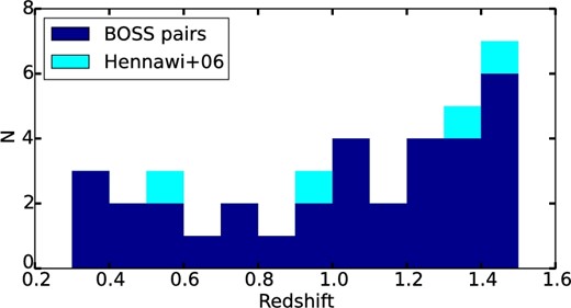
We extract our sample of low-redshift quasar pairs from the SDSS DR12Q catalog as follows. First, the selection area is limited to the ∼121 deg2 of the S16A effective area. Secondly, we limit the redshift range to z < 1.5, over which the photometric redshift estimate with the five-band photometry of the HSC has a large scatter and a high contamination rate (Tanaka et al. 2018). After applying the BOSS redshift flag (ZWARNING=0), we apply our definition of z ∼ 1 quasar pairs: two quasars within a projected separation R⊥ < 2 (=1.4 h−1) pMpc and velocity offset ΔV < 2300 km s−1. The maximum projected separation corresponds to the size of a z ∼ 1 proto-cluster, the descendant halo mass of which is Mhalo, z = 0 ∼ 1014 M⊙ (Chiang et al. 2013). It is chosen in order to select pairs with comparable separation to the two z > 3 pairs in this paper. The maximum velocity difference takes into account redshift uncertainty, peculiar velocity, and physical separation of <2 pMpc. At this stage, we select 38 pairs. We further require that the following positions and areas are within the S16A effective area to exclude insufficient fields for the overdensity measurements: (i) at the position of the quasars, (ii) at the pair center, (iii) over 70% of the 2 × 2 deg2 area centered on the pair, and (iv) over 80% of the pair vicinity (8 × 8 arcmin2). Finally, 33 pairs at 0.33 < z < 1.49 (z ∼ 1.02 on average) are extracted in the S16A area. Their redshift distribution is shown in figure 4. We find that J020332.82−050944.5 at z = 1.353 is double-counted, having two companions nearby. Since the projection separation of the two companions are over the cluster scale (i.e., >2 pMpc), we treat the two pairs individually in the following analysis. It is noted that whether these three quasars are considered as two pairs or a triplet does not affect our final result in section 5. In the search of 0.5 < z < 3 small-scale quasar pairs with the SDSS (Hennawi et al. 2006), two quasars with R⊥ < 1 h−1 pMpc and ΔV < 2000 km s−1 separation are assumed to be physically associated binaries. On the other hand, this study loosens the pair selection criteria, as we recognize a cluster-scale association of two quasars as a pair. While we have four small-scale (R⊥ < 1 pMpc) pairs from the BOSS catalog, it should be noted that our selection is not complete, since a complete search of such sub-pMpc-scale pairs requires a dedicated spectroscopic campaign. Detailed information on the pairs, such as coordinates, redshift, and pair separation, are given in table 4. Note that all z ∼ 1 pairs are in the W-XMMLSS region. We find that most of them are flagged as the BOSS ancillary program targets (ANCIALLY_TARGET2).
Quasar pairs at z ∼ 1 extracted from the BOSS DR12Q with their overdensity significance within two arcminutes.
| ID* | Redshift† | i ‡ | Δθ | R ⊥ | ΔV | |${\sigma}_{\mathrm{peak, 2^{\prime }}}{}^{\S }$| |
|---|---|---|---|---|---|---|
| [mag] | [″] | [pMpc] | [km s−1] | |||
| SDSS J020257.39−051225.4 | 0.512 | 21.13 ± 0.09 | 251.3 | 1.55 | 504 | 2.08 |
| SDSS J020313.15−051057.6 | 0.514 | 21.30 ± 0.10 | ||||
| SDSS J020320.47−050933.8 | 1.3526 | 21.18 ± 0.09 | 184.7 | 1.55 | 40 | 1.79 |
| SDSS J020332.82−050944.5‖ | 1.3529 | 21.10 ± 0.09 | ||||
| SDSS J020332.82−050944.5‖ | 1.3529 | 21.10 ± 0.09 | 182.7 | 1.54 | 1057 | 5.18 |
| SDSS J020341.74−050739.5 | 1.345 | 19.69 ± 0.05 | ||||
| SDSS J020334.58−051721.3♯ | 1.399 | 21.30 ± 0.11 | 99.9 | 0.84 | 130 | 1.62 |
| SDSS J020336.45−051545.4♯ | 1.400 | 20.42 ± 0.02 | ||||
| SDSS J020411.47−051032.7 | 0.326 | 19.86 ± 0.04 | 314.3 | 1.49 | 1261 | 1.39 |
| SDSS J020423.94−050619.6 | 0.332 | 19.74 ± 0.03 | ||||
| SDSS J020442.23−051041.3 | 1.329 | 20.90 ± 0.07 | 117.5 | 0.99 | 374 | 0.92 |
| SDSS J020448.12−050923.4 | 1.326 | 22.77 ± 0.32 | ||||
| SDSS J020645.57−044511.8 | 1.410 | 19.53 ± 0.07 | 226.6 | 1.91 | 2262 | 4.57 |
| SDSS J020700.09−044406.8 | 1.428 | 20.72 ± 0.08 | ||||
| SDSS J020659.51−042343.3 | 0.732 | 21.21 ± 0.08 | 173.0 | 1.26 | 587 | 2.94 |
| SDSS J020709.83−042501.5 | 0.729 | 21.32 ± 0.08 | ||||
| SDSS J021105.40−051424.0♯ | 1.078 | 21.37 ± 0.08 | 37.0 | 0.30 | 680 | 4.56 |
| SDSS J021107.88−051425.6♯ | 1.083 | 20.04 ± 0.04 | ||||
| SDSS J021335.21−055002.7 | 1.2219 | 18.86 ± 0.02 | 173.4 | 1.44 | 18 | 2.41 |
| SDSS J021339.82−055241.9 | 1.2220 | 20.56 ± 0.05 | ||||
| SDSS J021425.44−035631.7 | 1.423 | 20.63 ± 0.05 | 137.5 | 1.16 | 356 | 1.12 |
| SDSS J021434.30−035555.3 | 1.426 | 20.88 ± 0.05 | ||||
| SDSS J021436.80−045150.4 | 1.107 | 20.60 ± 0.21 | 156.6 | 1.28 | 1091 | 1.34 |
| SDSS J021444.98−045012.6 | 1.115 | 21.50 ± 0.10 | ||||
| SDSS J021448.84−040601.7 | 0.4447 | 20.22 ± 0.04 | 293.4 | 1.68 | 74 | 1.83 |
| SDSS J021508.19−040513.6 | 0.4451 | 20.07 ± 0.03 | ||||
| SDSS J021606.59−040508.4 | 1.1447 | 20.19 ± 0.13 | 147.3 | 1.21 | 26 | −0.11 |
| SDSS J021614.95−040626.3 | 1.1449 | 21.40 ± 0.08 | ||||
| SDSS J021610.64−045229.8 | 0.9570 | 21.35 ± 0.07 | 240.7 | 1.91 | 28 | 3.43 |
| SDSS J021626.53−045308.3 | 0.9568 | 21.17 ± 0.07 | ||||
| SDSS J021650.21−040142.6 | 1.031 | 20.96 ± 0.06 | 218.3 | 1.76 | 154 | 2.85 |
| SDSS J021659.43−035853.4 | 1.030 | 21.77 ± 0.11 | ||||
| SDSS J021710.20−034101.2 | 1.425 | 20.85 ± 0.07 | 178.1 | 1.50 | 296 | 1.37 |
| SDSS J021718.77−033857.6 | 1.427 | 21.59 ± 0.13 | ||||
| SDSS J021756.83−035316.6 | 0.7511 | 20.53 ± 0.04 | 231.2 | 1.70 | 92 | 4.20 |
| SDSS J021806.76−035019.5 | 0.7505 | 21.72 ± 0.13 | ||||
| SDSS J021757.23−050216.3 | 1.088 | 20.47 ± 0.04 | 237.0 | 1.93 | 1081 | 6.46 |
| SDSS J021809.48−045945.8 | 1.095 | 21.60 ± 0.10 | ||||
| SDSS J021809.55−050200.3 | 1.277 | 21.22 ± 0.07 | 128.3 | 1.07 | 1290 | 3.96 |
| SDSS J021817.20−050258.7 | 1.287 | 20.26 ± 0.04 | ||||
| SDSS J022024.49−040017.2 | 0.812 | 21.58 ± 0.11 | 228.2 | 1.72 | 1723 | 0.75 |
| SDSS J022032.41−040332.2 | 0.822 | 20.77 ± 0.06 | ||||
| SDSS J022125.05−055638.0♯ | 0.585 | 20.59 ± 0.04 | 150.4 | 0.99 | 893 | 2.98 |
| SDSS J022128.77−055857.7♯ | 0.580 | 19.81 ± 0.02 | ||||
| SDSS J022226.84−041313.4 | 1.486 | 21.73 ± 0.11 | 189.7 | 1.60 | 1193 | 1.73 |
| SDSS J022237.88−041140.3 | 1.496 | 21.52 ± 0.09 | ||||
| SDSS J022248.98−044824.6 | 1.419 | 20.81 ± 0.06 | 200.7 | 1.69 | 263 | 1.97 |
| SDSS J022253.17−044513.9 | 1.421 | 21.17 ± 0.09 | ||||
| SDSS J022534.82−042401.6 | 0.920 | 21.06 ± 0.08 | 152.8 | 1.20 | 222 | 5.90 |
| SDSS J022537.16−042132.9 | 0.921 | 19.32 ± 0.03 | ||||
| SDSS J022542.41−051452.4 | 1.258 | 21.35 ± 0.11 | 194.8 | 1.63 | 281 | 1.82 |
| SDSS J022554.86−051354.6 | 1.256 | 20.08 ± 0.04 | ||||
| SDSS J022550.97−040247.4 | 1.448 | 21.14 ± 0.08 | 150.1 | 1.27 | 799 | 2.25 |
| SDSS J022552.15−040516.5 | 1.441 | 21.30 ± 0.08 | ||||
| SDSS J022855.35−051130.6 | 0.366 | 18.97 ± 0.05 | 200.5 | 1.02 | 96 | 0.78 |
| SDSS J022855.95−051450.8 | 0.365 | 19.96 ± 0.06 | ||||
| SDSS J022916.82−044600.7 | 0.612 | 20.35 ± 0.04 | 193.9 | 1.31 | 455 | 1.60 |
| SDSS J022928.73−044444.0 | 0.610 | 20.53 ± 0.05 | ||||
| SDSS J023035.82−052603.2♯ | 0.364 | 19.68 ± 0.03 | 153.2 | 0.78 | 318 | 1.84 |
| SDSS J023038.66−052336.0♯ | 0.363 | 19.96 ± 0.03 | ||||
| SDSS J023231.43−053655.9 | 1.098 | 20.92 ± 0.07 | 165.5 | 1.35 | 408 | 3.18 |
| SDSS J023238.46−053903.9 | 1.101 | 21.01 ± 0.07 | ||||
| SDSS J023323.39−042803.0 | 1.238 | 21.41 ± 0.08 | 118.1 | 0.98 | 362 | 2.42 |
| SDSS J023331.24−042815.2 | 1.241 | 20.76 ± 0.06 | ||||
| SDSS J023328.44−054604.4♯ | 0.494 | 20.31 ± 0.03 | 41.1 | 0.25 | 170 | 2.46 |
| SDSS J023331.05−054550.9♯ | 0.493 | 18.45 ± 0.02 |
*DR12Q ID.
†DR12Q redshift (Z_VI).
‡SDSS-i PSF magnitude.
§Peak significance within two arcminutes around the pairs.
‖The quasar has two companions.
♯Small-scale pairs with R⊥ < 1 pMpc.
4.1.2 Pairs in literature
To complement the sub-pMpc-scale quasar pairs lacking in the BOSS pair selection, spectroscopically confirmed small-scale pairs identified in the literature are added to our sample. Such pairs are usually identified as by-products of lensed quasar searches. We look for spectroscopically confirmed binary quasars within the DR S16A coverage referring to the following literature: Djorgovski (1991), Hennawi et al. (2006), Myers et al. (2008), Inada et al. (2012), Kayo and Oguri (2012), More et al. (2016), and Eftekharzadeh et al. (2017). Following the same selection procedure applied to the BOSS quasars, we are able to measure the galaxy overdensity around four small-scale quasars originally identified in Hennawi et al. (2006). Therefore, the total number of quasar pairs including pairs from literature is 37, nine of which are R⊥ < 1 pMpc pairs. The redshifts of the additional pairs are shown in cyan in figure 4, and their properties are listed in table 5. The projected separation of the four pairs is almost comparable to the BOSS pairs, but SDSS J1152−0030 (z ∼ 0.55) has the smallest projected separation, R⊥ = 0.13 pMpc (Δθ = 29|${^{\prime\prime}_{.}}$|3), among our sample.
Quasar pairs at z < 1.5 from Hennawi et al. (2006).*
| ID | Redshift | i | Δθ | R ⊥ | ΔV | |${\sigma }_{\mathrm{peak, 2^{\prime }}}$| |
|---|---|---|---|---|---|---|
| [mag] | [″] | [pMpc] | [km s−1] | |||
| SDSS J1152−0030A | 0.550 | 18.80 ± 0.02 | 29.3 | 0.19 | 740 | 5.07 |
| 2QZ J1152−0030B | 0.554 | 19.99 ± 0.03 | ||||
| 2QZ J1209+0029A | 1.319 | 20.26 ± 0.04 | 165.8 | 1.39 | 340 | 0.94 |
| 2QZ J1209+0029B | 1.322 | 20.76 ± 0.05 | ||||
| 2QZ J1411−0129A | 0.990 | 19.85 ± 0.04 | 152.5 | 1.22 | 1820 | 1.14 |
| 2QZ J1411−0129B | 0.978 | 19.75 ± 0.03 | ||||
| 2QZ J1444+0025A | 1.460 | 20.34 ± 0.04 | 113.3 | 0.96 | 1950 | 0.43 |
| 2QZ J1444+0025B | 1.444 | 20.35 ± 0.04 |
*ID, redshift, separation are derived from their measurements converted with the cosmology we adopt. The i-band magnitudes are the extinction-corrected PSF magnitudes derived from the SDSS DR12. In the last column, we report the peak significance within two arcminutes around the pair center.
4.2 z ∼ 1 single quasars
To make a comparison with the z ∼ 1 pairs, we also measure the overdensity around single quasars at 0.9 < z < 1.1 in the W-XMMLSS region. To extract only isolated quasars, we require that there is no neighborhood quasar at R⊥ < 4 pMpc and ΔV < 3000 km s−1, in addition to the BOSS redshift flag. We set this boundary larger than the maximum pair separation to remove companion quasars associated with quasar pairs. We also check if their fields are suitable for overdensity measurements using the same criteria applied to the quasar-pair fields. As a result, 127 isolated quasars at z ∼ 1 are extracted, the sample size of which is large enough to be compared statistically with the pair environments.
4.3 z ∼ 1 galaxy selection
4.4 Random fields around z ∼ 1 galaxies
To compare the pair fields with the single-quasar fields, we compute the peak significance distribution around randomly selected z ∼ 1 galaxies. For this purpose, the random fields should be independent of the quasar presence. We make use of the 2 × 2 deg2 fields around the 127 single quasars at 0.9 < z < 1.1, and galaxies selected by the photometric redshift selection in subsection 4.3 (i.e., i < 24). We assume no significant redshift evolution of the surface galaxy density within 0.3 < z < 1.4. In each of the 127 fields, we randomly pick up 10 galaxies, removing the masked regions, the central 30 × 30 arcmin2 around quasars, and <15΄ at the edges. We then measure the significance peak within the two-arcminute radius to quantify the overdensity of the selected regions. We require that there is no overlap between each aperture centered at the randomly selected galaxies to ensure the independence of the selected regions. A certain amount of the 2 × 2 deg2 fields overlap, but this does not affect the randomness of the galaxy selection unless the selected galaxies are in the vicinity of others. After examining the randomly selected positions of the galaxies to check for any overlaps of the two-arcminute aperture with others, we finally derive the overdensity significance distribution around z ∼ 1 galaxies from 849 random fields, which is sufficient to compare the significance distribution of random fields with that of the quasar fields.
5 Result II: z ∼ 1 quasar-pair environments
5.1 Significance distribution
In this section, we show the result of the overdensity measurements in z ∼ 1 quasar-pair fields. Since we have an unprecedentedly large number of quasar pair samples, we are able to examine the rare pair environments with statistical approaches for the first time. Figure 5 shows the normalized distribution of the peak significance around the pairs. Globally, the peak significance distributes around a moderate density with the median significance of |$\langle \sigma _\mathrm{peak,2^{\prime }}\rangle =1.97$|. This result suggests that the quasar pairs at low redshift reside in moderate environments as a whole, in contrast to the high-redshift pairs. This is consistent with the findings of previous works (e.g., Boris et al. 2007; Sandrinelli et al. 2014), in which the authors do not find strong evidence that the local galaxy density is highly enhanced around z ≲ 1 pairs. However, it is notable that the distribution has a long tail toward high significance up to 6.46σ. To be specific, there are seven pairs (19%) with |$\sigma _\mathrm{peak,2^{\prime }}>4$|, including SDSS J1152−0030, the pair with the smallest projected separation (|$\sigma _\mathrm{peak,2^{\prime }}=5.07$|), and J020332−050944 and J020341−0500739, which has a companion (|$\sigma _\mathrm{peak,2^{\prime }}=5.18\sigma$|). These >4σ pair fields were visually checked to confirm that the overdense regions are not fakes due to, for example, false detections of artificial noises around bright stars. Their local significance maps are shown in figure 6, where it is clear that the significance is highly enhanced between or on the pair members. The maps of the other pairs hosted in normal- or under-density regions are shown later in figure 9 (see the Appendix). We also show the peak significance in the R∥–R⊥ plane in figure 7, where R∥ is the line-of-sight separation directly converted from the velocity difference ΔV. The significance is divided into three bins: |$4<\sigma _\mathrm{peak,2^{\prime }}$|, |$2< \sigma _\mathrm{peak,2^{\prime }}\le 4$|, and |$\sigma _\mathrm{peak,2^{\prime }}\le 2$|, with filled symbols showing the BOSS pairs and open symbols showing the Hennawi et al. (2006) pairs. The number of pairs in each bin and the number of sub-pMpc-scale pairs are summarized in table 6.
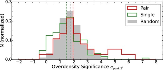
Normalized distribution of the overdensity significance around z < 1.5 quasar pairs (red), z ∼ 1 single quasars (green), and random galaxy fields (grey). The overdensity significance |$\sigma _\mathrm{peak, 2^{\prime }}$| is defined as the peak significance within a two-arcminute radius from quasars or galaxies. The pair center is used for the case of quasar pairs. The negative significance means that all the area inside the two-arcminute radius have smaller galaxy densities than the average. The median value for each distribution (pair: 1.97; single: 1.47; random: 1.75σ) is indicated with a vertical line. (Color online)

Local significance maps for seven z ∼ 1 pairs with >4σ overdensity within two arcminutes. The symbols and contours are the same as figure 1. The first six panels show the BOSS binary fields and the bottom panel shows the one from Hennawi et al. (2006). The white star in J020332−050944 and J020341−050739 field shows the companion quasar (SDSS J020320.47−050933.8) at z = 1.353. (Color online)
![Distribution showing the radial separation R∥ [pMpc] and projected separation R⊥ [pMpc] of the 37 pairs at z ∼ 1. The radial separation R∥ is converted from the velocity offset ΔV [km s−1] assuming z = 1, which is also shown for reference. The color shows the peak significance within two arcminutes, $\sigma _\mathrm{peak,2^{\prime }}$, in red ($4\le \sigma _\mathrm{peak,2^{\prime }}$), green ($2\le \sigma _\mathrm{peak,2^{\prime }}<4$) and blue ($\sigma _\mathrm{peak,2^{\prime }}<2$). The filled symbols show the BOSS quasar pairs. The open symbols show the pairs from Hennawi et al. (2006). (Color online)](https://oup.silverchair-cdn.com/oup/backfile/Content_public/Journal/pasj/70/SP1/10.1093_pasj_psx092/2/m_pasj_70_sp1_s31_f7.jpeg?Expires=1749144192&Signature=ZIFsi2RiNzR8UlckyfQX4wH51bNNxZFxiH1E0YIYfkAUcCJKC1y6DK4hfRYSi5q6x5QKnLkA1WoJsDtxOWtU6664IYnMBo9ZYaKuhaNJ0hauMNP7brWUErCXnSHFQqRkR7lViN-CbnKAXGjqy2OlVoiOUo9CqFg2vSUOZGpZ3rnQmzPtFdqmK0TFVFXmMPQEhpwmbE0Cbd9gH5Swrx5ATwWXiB8QbDC8qDunSc8kwEbz9nyIJG0ZKJjSYByO7JWgEi05Wv2-Q7SCYN5mc4rzjlFmJLCi--jcD0Fax9GOiaudH958hHi3mVh1XJyVx40IDEquCJzn3gAIazlGpzPECA__&Key-Pair-Id=APKAIE5G5CRDK6RD3PGA)
Distribution showing the radial separation R∥ [pMpc] and projected separation R⊥ [pMpc] of the 37 pairs at z ∼ 1. The radial separation R∥ is converted from the velocity offset ΔV [km s−1] assuming z = 1, which is also shown for reference. The color shows the peak significance within two arcminutes, |$\sigma _\mathrm{peak,2^{\prime }}$|, in red (|$4\le \sigma _\mathrm{peak,2^{\prime }}$|), green (|$2\le \sigma _\mathrm{peak,2^{\prime }}<4$|) and blue (|$\sigma _\mathrm{peak,2^{\prime }}<2$|). The filled symbols show the BOSS quasar pairs. The open symbols show the pairs from Hennawi et al. (2006). (Color online)
Summary of z ∼ 1 pair environments.*
| |$N_{4\le \sigma _\mathrm{peak, 2^{\prime }}}$| | |$N_{2\le \sigma _\mathrm{peak, 2^{\prime }}<4}$| | |$N_{\sigma _\mathrm{peak, 2^{\prime }}<2}$| | N total | |
|---|---|---|---|---|
| R ⊥ < 1 | 2 | 3 | 4 | 9 |
| R ⊥ ≥ 1 | 5 | 8 | 15 | 28 |
| |$N_{4\le \sigma _\mathrm{peak, 2^{\prime }}}$| | |$N_{2\le \sigma _\mathrm{peak, 2^{\prime }}<4}$| | |$N_{\sigma _\mathrm{peak, 2^{\prime }}<2}$| | N total | |
|---|---|---|---|---|
| R ⊥ < 1 | 2 | 3 | 4 | 9 |
| R ⊥ ≥ 1 | 5 | 8 | 15 | 28 |
*The overdensity significance of the 37 z ∼ 1 pair fields are divided by the projected separation of the pair (R⊥ < 1 and R⊥ ≥ 1 [pMpc]).
In figure 5, we also compare the significance distribution with those of single quasars and randomly selected galaxies. As the median significances are 1.47σ and 1.75σ, the overall significant distributions are only different by <1σ level from the pairs. However, a major difference is at the high-density outskirt, where the significance distributions of single quasars and galaxies decline smoothly, with the fraction of >4σ significance regions 2.4% and 2.0%, respectively. Taking advantage of the large sample size, we perform two-sample tests of goodness-of-fit to compare the three distributions. In all tests, the null hypothesis is that two non-parametric distributions are from the same underlying distribution. The significance threshold is set at 0.05. Three combinations of the pairs (P), single quasars (S), and random fields (R) distributions are tested as we summarize in table 7. First, the Kolmogorov–Smirnoff (KS) test (Smirnov 1939) shows that we cannot reject the possibility that any of the three samples come from the same distribution, implicating that there seems to be no significant levels of overdensity enhancement in pair- and single-quasar fields in a global view. On the other hand, from the Anderson–Darling (AD) test (Stephens 1974), which is more sensitive to the tail of the distribution, it is statistically supported that the pair environments are more likely to be overdense. Moreover, comparing with the two quasar groups (“P–S” in table 7), we find that quasar pairs favor cluster environments. Intriguingly, it is also evident that the single quasar fields are likely underdense, compared with the galaxy fields. Since the two pairs at z = 3.3 and 3.6 have physical separations comparable to the z ∼ 1 pairs, our result suggests that <2 pMpc-scale quasar pairs are good tracers of massive clusters both at z > 3 and z ∼ 1, yet the probability of finding clusters seems smaller at low redshift.
Two-sample KS and AD test.*
| KS | AD | ||||
|---|---|---|---|---|---|
| D | p | A 2 | p | ||
| P–R | 0.30 | 0.28 | 5.1 | 0.0033 | |
| S–R | 0.20 | 0.77 | 9.8 | 0.0001 | |
| P–S | 0.30 | 0.28 | 6.3 | 0.0014 | |
| Pz1.0–Pz1.5 | 0.20 | 0.77 | −1.0 | 1.0 | |
| KS | AD | ||||
|---|---|---|---|---|---|
| D | p | A 2 | p | ||
| P–R | 0.30 | 0.28 | 5.1 | 0.0033 | |
| S–R | 0.20 | 0.77 | 9.8 | 0.0001 | |
| P–S | 0.30 | 0.28 | 6.3 | 0.0014 | |
| Pz1.0–Pz1.5 | 0.20 | 0.77 | −1.0 | 1.0 | |
*“P” represents the quasar pairs, while “S” and “R” represent the single quasars at 0.9 < z < 1.1 and the random sample as described in subsection 4.4. For example, “P–S” stands for the comparison of the pair and single quasars. “Pz1.0–Pz1.5”is the comparison of the pairs divided into two groups: z < 1.0 and 1.0 ≤ z < 1.5. The test statistics are shown in D and A2 with corresponding p-values.
5.2 Significance dependence on redshift
Here, we examine the redshift dependence, albeit in a narrow range, of the peak significance of the pair environments. The pair sample is divided into (i) a z < 1.0 group and (ii) a 1.0 ≤ z < 1.5 group. There are 15 pair fields at z < 1 with median significance 2.08σ and 22 pair fields at 1 ≤ z < 1.5 with median significance 1.90σ. Figure 8 compares the normalized significance distributions of the two pair groups. After applying the two-sample tests, we find that there is no significant redshift-dependence of the peak significance (table 7). Note that this result supports our initial assumption that the pair environments do not significantly change at 0.3 < z < 1.5.
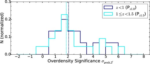
Normalized significance distribution of the z ∼ 1 pairs divided into z < 1.0 pairs (“Pz1.0”, blue) and 1.0 ≤ z < 1.5 pairs (“Pz1.5”, cyan). There are 15 pairs in Pz1.0 group and 22 pairs in Pz1.5 group. The grey histogram shows the random sample which is the same as in figure 5. (Color online)
6 Discussion
6.1 Enhancement of overdensity around z > 3 quasar pairs
In this study, we derive an implication that the rare occurrence of <2 pMpc-scale quasar pairs is related to galaxy overdensity regions at z > 3 and also, with a statistical evidence at z ∼ 1. At high redshift, if the effective projection size of a z ∼ 4 proto-cluster is defined as having a 1|${^{\prime}_{.}}$|8 (0.75 pMpc: Chiang et al. 2013) radius, the total surface area of the 179 HSC proto-clusters is 0.51 deg2, which is only 0.4% of the entire S16A field. Therefore, when one assumes a uniform surface density of quasar pairs, the chance that two randomly selected positions in 121 deg2 are both in proto-cluster fields is only 2 × 10⁻⁵, yet we find two proto-clusters out of the two pairs.
At this stage, we take a look again at the work of Uchiyama et al. (2018). Using the same HSC g-dropout selection and parent quasar catalog, they suggest that the majority of 151 quasars at z ∼ 3.8 likely reside in moderate-density environments. As also mentioned in section 3 in this paper, there are only six BOSS quasars located within three arcminutes (∼1.25 pMpc) of the density peaks of the HSC proto-clusters, and intriguingly, three of them are the QSOP1 and QSOP2 pair members (figure 1). While several studies argue high-redshift quasar environments with small-field observations, for example using the Hubble Space Telescope, the area used for the overdensity measurements in our HSC-SSP studies is sufficient to identify proto-clusters and to see their entire structures thanks to the enormously wide coverage. Thus, unlike the average environments of isolated quasars at z ∼ 3.8, it is assured that the two quasar-pair fields showing large excess (>5σ) of overdensity significance are exceptionally rare and rich as quasar environments at this epoch. In terms of the triggering mechanism, our result suggests that, even though the vast majority of luminous quasars may be triggered via the secular process, which is independent of the galaxy density, quasars that are turned on by the heavy interaction of massive galaxies do exist in massive haloes, and such quasar activity is perhaps so synchronous, especially at high redshift, that we observe more than one quasar in proto-clusters. This result supports our initial anticipation that pairs of luminous quasars are better tracers of proto-clusters than single quasars. Meanwhile, given that Fukugita et al. (2004) find no overdensity around a quasar pair at z = 4.25, while their imaging area is small (5.8 arcmin2), a bigger pair sample at z > 3 is needed to derive more conclusive evidence. Spectroscopic or narrow-band imaging follow-up observation of the two pair fields is required to address (i) the identification of member galaxies, (ii) the presence of quasars fainter than the one found in the QSOP2 field, and (iii) star-formation activity of the member galaxies.
It is notable that the two pair fields are not the richest among the HSC proto-clusters. Toshikawa et al. (2018) find up to 9σ overdensity regions, while the pair fields have 4.8 and 4.0σ in their measurements. The interpretation of this fact is not straightforward. The AGN feedback suppression of the quasar activity in the most massive haloes (Fanidakis et al. 2013; Orsi et al. 2015) could explain the absence of luminous quasars in the high-density regions, though it cannot explain why the QSOP1 and QSOP2 pair members can emerge in proto-clusters. A certain amount of quasars in proto-clusters could be missed in the incomplete selection of the BOSS catalog especially at z > 3.5, but it is unlikely that the members of the two quasar pairs pass the BOSS color selection but the majority of other quasars in other >100 proto-clusters do not. As an alternative explanation, AGN in the most massive haloes simply might not turn on in the more massive proto-clusters, if one takes into account the short AGN duty cycle of typically 107 yr. In this context, another possibility would be that the quasar activity is triggered in the massive haloes but they are not in the type-I quasar phase; thus they are not optically bright. Since we are just starting the proto-cluster search in the first ∼100 deg2, it would be of great interest to study the relation between the most overdense regions and luminous quasars with a larger sample size as the HSC-SSP survey coverage is enlarged. Furthermore, far-infrared or sub-mm studies of the HSC proto-clusters is necessary to probe obscured galaxies residing in proto-clusters.
We note that two sub-pMpc-scale quasar pairs in Hennawi et al. (2010), namely SDSS J1054+0215 at z ∼ 3.98 and SDSS J1118+0202 at z ∼ 3.94, are at our redshift range and within the entire HSC-Wide survey area, while these fields have not been covered yet. Also, CFHTLS J0221−0342, another small-scale pair at z = 5 reported in McGreer et al. (2016), is within the W-XMMLSS field covered with the HSC-Deep layer, but the current depth of that layer is almost the same as the Wide. We will investigate these small-scale pair environments at z > 3 after their fields are covered or the imaging gets deeper, to compare them with larger separation pairs like the two in this paper, as well as with the other pairs which will be covered in the future HSC-SSP data release, and also with the z ∼ 1 counterparts.
Finally, the environment around fainter z > 3 quasars is another important topic. While low-luminosity quasars are more easily triggered in normal environments as would also be the case for quasar pairs, such measurements will provide a clue to understand how the host haloes and surrounding galaxy overdensity affect the triggering mechanism of low-luminosity quasars. In the HSC-SSP, Akiyama et al. (2018) compile a >1000 sample of z ∼ 4 quasars down to i = 24 to derive the accurate shape of the quasar luminosity function at the faint end. He et al. (2018) discuss the clustering of their quasars to show that their host halo masses are moderate, with an order of Mhalo ∼ 1012M⊙. In order to asses their measurements from an environmental point of view, it is highly required to investigate the galaxy overdensity of their low-luminosity quasars.
6.2 Redshift-dependence of quasar-pair environments
Different environments between single quasars and pairs are also found at z ∼ 1; we show in section 5 that a significant fraction of quasar-pair fields is at high-density regions, which is statistically different from those of single quasars and randomly selected galaxies. However, a big difference from the z > 3 pair environments is that the significance distribution is globally the same among the three environments, meaning that quasars are generally common in any environments at z ∼ 1. Since the brightness of most z ∼ 1 quasars is in the range of 19 < i < 21 and this is the same for the pairs in >4σ regions, the brightness dependence of the pair environments does not have a major effect on the result.
The trend that not all z ∼ 1 quasar pairs reside in massive environments as well as single quasars is consistent with previous studies. For example, Farina, Falomo, and Treves (2011) show that, although the pair selection is severer than this study (i.e., R⊥ < 500 kpc and ΔV < 500 km s−1), only one out of six pair fields at z < 0.8 shows significant overdensity, using galaxies as bright as the ones in this study. Boris et al. (2007) adopt a loose pair selection at z ∼ 1 (Δθ < 300″) which is comparable to this study. They conduct a deep optical imaging observation with Gemini/GMOS down to the 1.5σ limit i΄ = 26.4 in four pair fields, showing that three pairs are associated with cluster environments but the other one is in an isolated field. Sandrinelli et al. (2014) stack the radial profile of galaxies in 14 pair fields at z < 0.85 (R⊥ < 600 kpc) and suggest that there is no clear enhancement of overdensity compared with that of single quasars. We note that the definition of overdensity and its significance are different between this and previous studies; therefore the probability of finding overdense regions around quasar pairs in previous works cannot be compared with this study. These results can be discussed under the downsizing evolution of the quasar activity. At high redshifts, quasar activity is most efficient in the most massive SMBHs residing in dense environments, for which plenty of cold gas is available for the mass growth to make gigantic SMBHs (MBH > 109M⊙) such as those found at z > 6 (e.g., Mortlock et al. 2011; Wu et al. 2015). At lower redshifts, the galaxy interaction becomes common in normal environments following the fast growth of SMBHs in proto-clusters. The luminosity where the quasar activity is most active shifts to a less-luminous range as quasars are powered by already-matured black holes or less-massive black holes in their late growth. The observational evidence of such anti-hierarchical evolution is given by, for instance, Ueda et al. (2014) in their X-ray AGN luminosity function over 0 < z < 5. In this respect, our result confirms the down-sizing trend of the SMBH growth by showing from an environmental point of view that the majority of low-redshift quasars, even for quasar pairs, turn on in moderate environments, in contrast to the z > 3 quasar pairs.
Furthermore, our measurement of >30 z ∼ 1 pair environments shows statistical evidence that (not all, but) ∼20% of the quasar pairs do reside in cluster fields, and this is distinguishable from the isolated quasar environments and random fields. This feature is found thanks to our large sample size, whereas previous studies are limited to ∼10 pair fields. The high-density tail in the significance distribution of the pairs suggests that the quasar activity is still ongoing in massive haloes and is actually so active at z ∼ 1 that more than one quasar is triggered at the same time. There should be isolated quasars in other massive environments, but they would not be visible since they are hidden by a larger number of quasars in moderate environments. The implication of this trend is that there are still remnants and further accretion of cold-gas in cluster environments even after the major epoch of star-forming and SMBH feeding, and the frequent galaxy interaction can ignite more than one quasar simultaneously.
There are nine quasar pairs with less than 1 pMpc projected separation including two from Hennawi et al. (2006). From the nine sub-pMpc-scale pairs, we find that two pairs, J021105−051424 and J021107−051425 at z ∼ 1.08 (R⊥ = 0.30 pMpc, ΔV = 680 km s−1), and J1152−0030A and B at z ∼ 0.55 (R⊥ = 0.19 pMpc, ΔV = 740 km s−1), are embedded in high-density environments (|$\sigma _\mathrm{peak,2^{\prime }}=4.56\sigma$| and 5.07σ, respectively). On the other hand, the significance of the other seven pairs is moderate or small (|$\sigma _\mathrm{peak,2^{\prime }}=0.4$|–3.0), like the larger-separation pairs. Therefore, while several studies on such small-scale clustering of quasars suggest that the clustering signal of a projected correlation function is enhanced from the extrapolation from Mpc-scale due to intense interaction of galaxies in massive haloes (Eftekharzadeh et al. 2017; Hennawi et al. 2006), our result implies that such small-scale quasar pairs are hosted not only in cluster fields but also in general fields at z ∼ 1.
7 Summary
In this paper, we investigate the galaxy overdensity of quasar-pair environments at high (z > 3) and low (z ∼ 1) redshift, using the optical imaging catalog of the HSC-SSP survey (DR S16A) covering effectively 121 deg2 with the i-band 5σ depth of ∼26.4. The quasar pairs are primarily extracted from the SDSS DR12Q catalog, with an additional sample from literature at z ∼ 1. We use the photometric catalog of the HSC-SSP to select surrounding galaxies based on our g-dropout selection at z > 3 and photometric redshift selection at z ∼ 1. The galaxy overdensity measurement around quasar pairs is based on the local significance of galaxies within a 1.8΄ aperture at each square grid over a 2 × 2 deg2 field separated by 0.6΄. Our main results are summarized as follows.
We find that two quasar pairs at z = 3.3 and 3.6 are associated with σpeak > 5σ overdensity regions. Their projection separations are R⊥ = 1.75 and 1.04 pMpc, and their velocity offsets are ΔV = 692 and 1448 km s−1, respectively. The number counts around the two pairs are about more than two times higher than those in field environments in all magnitude bins down to i = 26, and show further excess at the bright (i < 23) side. Since it has been found that there is no apparent trend that quasars at z ∼ 3.8 are related to massive environments, pairs of luminous quasars are likely more efficient tracers of proto-clusters than isolated quasars, although a bigger pair sample is needed to discuss the probability of tracing the high-density regions and its redshift dependence. Our result implies that the two quasar pairs are likely triggered via galaxy major merger, while the vast majority of isolated quasars are triggered via other processes such as bar and disk instabilities.
The overdensity significance of the z > 3 pair environments is not the highest among 179 HSC proto-clusters, which may imply that luminous quasars cannot emerge in the most massive haloes. However, this is not clear since we may miss quasars in the largest proto-clusters due to the incomplete selection of z > 3.5 quasars, and quasars may actually exist in the richest environments but they are not optically bright due to obscuration or their turn-off phase in the duty cycle.
We extend our study down to z ∼ 1 using the HSC-SSP photometric redshifts. We select 33 pairs from the BOSS DR12Q and also four previously known small-scale pairs from Hennawi et al. (2006). While the distribution of peak significance within two arcminutes from the pair center is not globally different from those of isolated quasars and randomly selected galaxies in the same redshift range, a significant difference is found at the high-density tail thanks to our large sample size. We find that 19% of the z ∼ 1 pairs are within massive (>4σ) environments and statistically confirm that this is unique in pair environments. Our result suggests that more than one quasar can ignite simultaneously in massive haloes even after the major epoch of the AGN activity, and quasar pairs are still good tracers of rich environments at z ∼ 1, while the chance is lower than at z > 3. We detect no redshift dependence of the significance between z < 1 pairs and 1 ≤ z < 1.5 pairs.
Among nine small-scale pairs with R⊥ < 1 pMpc, two of them reside in >4σ fields including the pair with the smallest projected separation, SDSS J1152−0030A and B (z ∼ 0.55, R⊥ = 0.19 pMpc). The other fields are moderate- or under-density regions, suggesting that sub-pMpc-scale pairs could be embedded in general fields at low-redshift like isolated quasars.
Acknowledgements
We thank the anonymous referee for helpful comments on the manuscript. MO would like to express gratitude to B. Venemans and E. P. Farina for fruitful discussions at the initiation of this work. MO acknowledges Roderik Overzier, Toshihiro Kawaguchi, and Satoshi Kikuta for their suggestive comments on the manuscript.
This work is based on data collected at the Subaru Telescope and retrieved from the HSC data archive system, which is operated by Subaru Telescope and Astronomy Data Center at National Astronomical Observatory of Japan.
The Hyper Suprime-Cam (HSC) collaboration includes the astronomical communities of Japan and Taiwan, and Princeton University. The HSC instrumentation and software were developed by the National Astronomical Observatory of Japan (NAOJ), the Kavli Institute for the Physics and Mathematics of the Universe (Kavli IPMU), the University of Tokyo, the High Energy Accelerator Research Organization (KEK), the Academia Sinica Institute for Astronomy and Astrophysics in Taiwan (ASIAA), and Princeton University. Funding was contributed by the FIRST program from Japanese Cabinet Office, the Ministry of Education, Culture, Sports, Science and Technology (MEXT), the Japan Society for the Promotion of Science (JSPS), Japan Science and Technology Agency (JST), the Toray Science Foundation, NAOJ, Kavli IPMU, KEK, ASIAA, and Princeton University.
This paper makes use of software developed for the Large Synoptic Survey Telescope. We thank the LSST Project for making their code available as free software at 〈http://dm.lsst.org〉.
The Pan-STARRS1 Surveys (PS1) have been made possible through contributions of the Institute for Astronomy, the University of Hawaii, the Pan-STARRS Project Office, the Max-Planck Society and its participating institutes, the Max Planck Institute for Astronomy, Heidelberg and the Max Planck Institute for Extraterrestrial Physics, Garching, The Johns Hopkins University, Durham University, the University of Edinburgh, Queen’s University Belfast, the Harvard-Smithsonian Center for Astrophysics, the Las Cumbres Observatory Global Telescope Network Incorporated, the National Central University of Taiwan, the Space Telescope Science Institute, the National Aeronautics and Space Administration under Grant No. NNX08AR22G issued through the Planetary Science Division of the NASA Science Mission Directorate, the National Science Foundation under Grant No. AST-1238877, the University of Maryland, and Eotvos Lorand University (ELTE) and the Los Alamos National Laboratory.
A part of this work is financially supported by the overseas internship fund of Department of Astronomical Science, SOKENDAI and JSPS KAKENHI Grant Number 15J02115. NK acknowledges supports from the JSPS KAKENHI Grant Number 15H03645.
Appendix. Low-density environments around z ∼ 1 quasar pairs
In section 5, we show that seven out of 37 z ∼ 1 quasar pairs are embedded in >4σ overdensity regions as shown in figure 6. Here, we show the other 29 pair fields showing lower (|$\sigma _\mathrm{peak,2^{\prime }}<4$|) overdensity significance for reference in figure 9, in which their redshift, pair separation (R⊥ and ΔV), and peak significance |$\sigma _\mathrm{peak,2^{\prime }}$| are given. Note that J020320−050933 and J020332−050944, the companion pair of J020332−050944 and J020341−050739 at z ∼ 1.35, is shown in the top left-hand panel of figure 6.


Local significance maps of the 30 pair fields showing |$\sigma _\mathrm{peak,2^{\prime }}<4\sigma$|. The symbols and contours are the same as figure 6. The first 27 panels show the BOSS pairs (see table 4), and the last three are the Hennawi et al. (2006) pairs (see table 5). Note that one field, J020320−050933 and J020332−050944-050944, is shown in the panel in figure 6 (the first panel at the top left). (Color online)
Footnotes
The 5σ-limiting magnitude is defined as the point where the PSF magnitude has S/N ∼ 5σ at 0 |${^{\prime\prime}_{.}}$|5–0 |${^{\prime\prime}_{.}}$|7 seeing condition. See Aihara et al. (2018b).
Specifically, we use the following flags: centroid_sdss_flags, flags_pixel_edge, flags_pixel_interpolated_center, flags_pixel_saturated_center, flags_pixel_cr_center, flags_pixel_bad, flags_pixel_suspect_center, cmodel_flux_flags.
The pair vicinity is excluded in the calculation of the field number counts.
Specifically, we use photoz_prob_star<0.1 for removing Galactic stars, reduced_chisq<10 for removing sources with unusual optical SEDs, and photoz_conf_median>0.2 for removing sources with flat P(z) distribution.
References
