


Abstract
We have measured the clustering of galaxies around active galactic nuclei (AGNs) for which single-epoch virial masses of the super-massive black hole (SMBH) are available to investigate the relation between the large-scale environment of AGNs and the evolution of SMBHs. The AGN samples used in this work were derived from the Sloan Digital Sky Survey (SDSS) observations and the galaxy samples were from the 240 deg2 S15b data of the Hyper Suprime-Cam Subaru Strategic Program (HSC-SSP). The investigated redshift range is 0.6–3.0, and the masses of the SMBHs lie in the range 107.5–1010 M⊙. The absolute magnitude of the galaxy samples reaches to Mλ310 ∼ −18 at rest-frame wavelength 310 nm for the low-redshift end of the samples. More than 70% of the galaxies in the analysis are blue. We found a significant dependence of the cross-correlation length on redshift, which primarily reflects the brightness-dependence of the galaxy clustering. At the lowest redshifts the cross-correlation length increases from 7 h−1 Mpc around Mλ310 = −19 mag to >10 h−1 Mpc beyond Mλ310 = −20 mag. No significant dependence of the cross-correlation length on BH mass was found for whole galaxy samples dominated by blue galaxies, while there was an indication of BH mass dependence in the cross-correlation with red galaxies. These results provides a picture of the environment of AGNs studied in this paper being enriched with blue star-forming galaxies, and a fraction of the galaxies are evolving into red galaxies along with the evolution of SMBHs in that system.
1 Introduction
Most galaxies have a supermassive black hole (SMBH) with mass greater than ∼ 106 M⊙ at their center (Richstone et al. 1998). Observations of the local Universe have revealed that the mass of the SMBH correlates with the several properties of the bulge component of the host galaxy (Magorrian et al. 1998; Ferrarese & Merritt 2000; Gebhardt et al. 2000; Ho 2007). This observational evidence suggests that a SMBH and its host galaxy co-evolve in a coordinated way in spite of the nine orders of difference in their physical size scale (Kormendy & Ho 2013).
SMBHs grow through the accretion of gas from their host galaxies or large-scale environment. Accretion in a secular mode, which arises through internal dynamical processes such as bar or disk instability or external processes driven by galaxy interaction, is one of the mechanisms to deliver the gas into the SMBH (Kormendy & Kennicutt 2004). As the mass accretion rate of the secular mode cannot be as high as to maintain the activity seen in bright quasi-stellar objects (QSOs) (Menci et al. 2014), this mode could operate in lower-luminosity active galactic nuclei (AGNs).
A merger of galaxies can induce gravitational torques which drive inflows of cold gas toward the center of galaxies (e.g., Hopkins et al. 2008). Observational evidence has been obtained that shows the relation between AGN activity and a galaxy merger (e.g., Sanders et al. 1988; Treister et al. 2012). The activity of the bright QSOs could be explained by this model. Although the accretion can be at its most efficient mode, it is also expected that AGN feedback promptly operates and stops the gas inflows when the mass of the SMBH becomes as large as 109 M⊙ (Fanidakis et al. 2013).
As an alternative process to make a SMBH evolve above 109 M⊙, quiescent gas accretion from the hot halo (Kereš et al. 2009; Fanidakis et al. 2013) and/or recycled gas from evolving stars (Ciotti & Ostriker 2001, 2007) has been proposed. According to the predictions of semi-analytical modeling by Fanidakis et al. (2013), AGNs fueled in the hot-halo mode are located in more massive dark matter halos than the AGNs fueled in the merger-driven starburst mode.
The mass of the host dark matter halo that AGNs reside in can be inferred from the auto-correlation function of AGNs at distance scale >1 Mpc. According to the analysis of auto-correlation of SDSS QSOs by Ross et al. (2009), the halo mass is almost constant at ∼ 2 × 10¹² h − 1 M⊙ in the redshift range from 0.3 to 2.2. It is also possible to estimate the halo mass from the cross-correlation between AGNs and galaxies if the auto-correlation functions of galaxies are precisely obtained. According to the cross-correlation
studies, the dark matter halo mass is estimated to be 1012–1013.5 h − 1 M⊙ depending on the detection wavelength of the AGNs (e.g., Hickox et al. 2009; Krumpe et al. 2012). Studies on clustering and/or environments of AGNs have also been reported elsewhere (e.g., Croom et al. 2005; Coil et al. 2009; Silverman et al. 2009; Donoso et al. 2010; Allevato et al. 2011; Bradshaw et al. 2011; Shen et al. 2013; Mountrichas et al. 2013; Zhang et al. 2013; Georgakakis et al. 2014; Krumpe et al. 2015; Ikeda et al. 2015).
Although the number of AGN clustering studies published so far is large, the studies focused on the relation between the mass of the central BH, which is the most fundamental property on which the history of mass accretion is imprinted, and also the properties of galaxies such as color and luminosity function around it are very limited. Since the interaction in the scale of groups or clusters of galaxies can induce concurrent activities of star formation, mass accretion to the central BH, and transition to the red sequence in the constituent galaxies, the contribution of such large-scale phenomena to the evolution of SMBHs can be inferred from the surrounding galaxies.
Shen et al. (2009) measured the clustering of QSOs for samples divided by their BH mass at redshifts 0.4–2.5 and did not find significant dependence, except for the most massive sample, for which marginally larger clustering was found on the ∼2σ level. Komiya et al. (2013) examined the dependence of the AGN–galaxy clustering on the BH mass at a redshift range from 0.3 to 1.0 using the UKIRT Infrared Deep Sky Survey (UKIDSS) data for the galaxy samples, and found that the cross-correlation length increases above 108.2 M⊙. Krolewski and Eisenstein (2015) also examined the BH mass dependence of the AGN–galaxy clustering at redshift ∼0.8 using Sloan Digital Sky Survey (SDSS) and Wide-field Infrared Survey Explorer (WISE) data for the galaxy samples, and found no significant relationship between clustering amplitude and BH mass. Krumpe et al. (2015) measured clustering of soft X-ray and optically selected AGNs at redshifts from 0.16 to 0.36 and detected a weak dependence on the mass at a significance level of 2.7σ, while they didn’t detect significant dependence on the Eddington ratio. They conclude that the mass dependence is the origin of the observed weak X-ray luminosity clustering dependence.
Extending the data set of Komiya et al. (2013), Shirasaki et al. (2016) derived, for the first time using a statistically significant number of samples, color and absolute magnitude distributions of galaxies around AGNs, and found that the increase of the cross-correlation length found by Komiya et al. (2013) is due to the increase in the number density of red galaxies. Those results indicate that the most massive SMBHs are evolved in dark matter halos more massive than the lower-mass SMBHs, and the surrounding galaxies also evolve in a coordinated way with the SMBHs which are mostly located in the center of host halo. To extend further the study given in Shirasaki et al. (2016) up to redshifts ∼3, which covers the era of the peak of star formation and mass accretion rate for SMBHs, we require a deeper wide multi-band survey.
The Hyper Suprime-Cam Subaru Strategic Program (HSC-SSP) is a multi-band imaging survey conducted with the HSC on the 8.2 m Subaru Telescope. The survey consists of three layers: Wide (1400 deg2, r ∼ 26), Deep (27 deg2, r ∼ 27), and UltraDeep (3.5 deg2, r ∼ 28). The HSC-SSP Wide survey provides the first opportunity to investigate the environment of AGNs up to redshift three with unprecedented statistics. Using the unique data set of the HSC-SSP Wide survey, this paper’s purpose is to measure not only the clustering of galaxies around AGNs but also their color and luminosity distribution as a function of SMBH mass at five redshift groups from 0.6 to 3.0. The results obtained in this work will give us a unified picture of evolution of galaxies and SMBHs under the large-scale structure of the Universe at their most important stage.
Throughout this paper, we assume a cosmology with Ωm = 0.3, Ωλ = 0.7, h = 0.7, and σ8 = 0.8. All magnitudes are given in the AB system. All the distances are measured in comoving coordinates. The correlation length is presented in unit of h−1 Mpc. The group and parameter names that are frequently refereed to in the text are summarized in table 11 of the Appendix.
2 Data sets
2.1 AGNs
The AGN samples used in this paper were drawn from the QSO properties catalog of Shen et al. (2011, hereafter S11) and the SDSS DR12 Quasar catalog (DR12Q) of Pâris et al. (2017). We used the S11 catalog as a reference for the BH mass estimate so as to be consistent with the previous studies (Komiya et al. 2013; Shirasaki et al. 2016), and the BH masses derived from the DR12Q catalog and spectral measurements were calibrated with those derived in S11.
To check the consistency between the BH masses derived by different relations, we compared them for the same objects. The left-hand panel in figure 1 shows the comparison of BH masses given in S11, |$M_{\rm BH,Mg\, {\small{II}}}$|(S11), and those calculated for the same object in DR12Q, |$M_{\rm BH,Mg\,{\small{II}}}$|(DR12Q), using equation (1). We found there is a systematic offset of 0.24 dex and scatter of 0.22, so we have corrected for the offset to the mass calculated using equation (1).
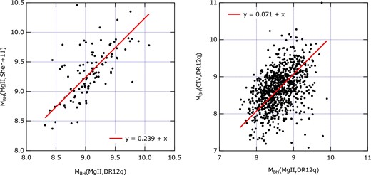
Comparisons of BH masses derived by different methods for the same object. Left-hand panel shows the comparison between the BH masses as given in S11 (Shen et al. 2011) and those calculated for the same object in DR12Q (Pâris et al. 2017) using equation (1). Right-hand panel shows the comparison between the BH masses calculated for an object in DR12Q using equation (1) and (2). The solid lines represent linear expressions fitted to the data points. (Color online)
The right-hand panel in figure 1 shows the comparison of BH masses calculated for objects in DR12Q using equation (1), |$M_{\rm BH,Mg\, {\small{II}}}$|(DR12Q), and equation (2), |$M_{\rm BH,C\, {\small{IV}}}$|(DR12Q). A systematic offset of 0.07 dex and scatter of 0.48 dex were found between them. Thus the offset of |$M_{\rm BH,C\, {\small{IV}}}$|(DR12Q) to |$M_{\rm BH,Mg\, {\small{II}}}$|(S11) was estimated to be 0.17, and the corresponding correction was made to |$M_{\rm BH,C\, {\small{IV}}}$|(DR12Q). As mentioned in Mejia-Restrepo et al. (2016) and is apparent from figure 1, |$M_{\rm BH,C\, {\small{IV}}}$| has a larger uncertainty than the mass measured based on other emission lines, so we used MBH, Mg ii, whenever it was available, as a mass estimator prior to |$M_{\rm BH,C\,\small{IV}}$|. The AGN samples for which BH mass is estimated from the |$C\,\small{IV}$| line are mostly at z ≥ 2.3. The effect of the large uncertainty of the C iv BH mass is limited only to the results for z ≥ 2.0.
Coatman et al. (2017) recently showed that an empirical correction to C iv BH masses based on the blueshift of the C iv emission line reduces the uncertainty. To apply the correction requires an accurate measure of the AGN systemic redshift. Thus, we decided to use the relation of equation (2) which does not require precise spectroscopic measurements.
The systematic offset and scatter between MBH, H β and |$M_{\rm BH, Mg\, {\small{II}}}$| given in the S11 catalog are 0.009 dex and 0.38 dex, respectively, as shown in figure 10 of Shen et al. (2011). Thus, no correction to MBH, H β is required.
For AGNs appearing in both catalogs, we used the redshift and BH mass of the S11 catalog. The redshift range of the AGNs was chosen to be 0.6–3.0, so that it overlaps with the highest redshift bin (z = 0.6–1.0) of the previous studies (Komiya et al. 2013; Shirasaki et al. 2016), in order to cross-check between both the results and extend up to the limit of sensitivity of this analysis. The BH mass range was set to 107–1011 M⊙. We selected 6166 AGNs which are in the redshift and BH mass ranges and are located within the footprint of HSC-SSP Wide survey.
2.2 Galaxies
The galaxy sample was collected from the HSC-SSP S15b Wide survey data set. HSC-SSP is a three-layered, multi-band (grizy plus four narrow-band filters) imaging survey made with the HSC (Miyazaki et al. 2012, 2018) on the 8.2 m Subaru Telescope. The total area and the depth of observation will be 1400 deg2 with r ∼ 26 (Wide layer), 27 deg2 with r ∼ 27 (Deep layer), and 3.5 deg2 with r ∼ 28 (UltraDeep layer).
We used the data set derived from the Wide layer. The observed locations and effective area are summarized in table 1. The typical depths of the observation are 26.8, 26.4, 26.4, 25.5, 24.7 for the g, r, i, z, and y bands, respectively. The detail of survey itself is described in Aihara et al. (2018b), and the content of the S15b data set is in Aihara et al. (2018a). The S15b data set was analyzed through the HSC pipeline (version 4.0.1) developed by the HSC software team using codes from the Large Synoptic Survey Telescope (LSST) software pipeline (Ivezic et al. 2008; Axelrod et al. 2010). The photometric and astrometric calibrations are made based on data obtained from the Panoramic Survey Telescope and Rapid Response System first imaging survey (Pan-STARRS1: Magnier et al. 2013; Schlafly et al. 2012; Tonry et al. 2012).
Summary of the survey area.
| Field name | Center coordinates | Si* | Sgriz † |
|---|---|---|---|
| RA, Dec (J2000.0) | (deg2) | (deg2) | |
| XMM-LSS | 02h18m, −04°30΄ | 51.8 | 48.9 |
| GAMA09H | 09h00m, +01°00΄ | 53.0 | 41.9 |
| WIDE12H | 11h58m, +00°00΄ | 32.5 | 24.6 |
| GAMA15H | 14h32m, +00°00΄ | 38.6 | 35.4 |
| HECTOMAP | 16h24m, +43°30΄ | 9.6 | 9.0 |
| VVDS | 22h24m, +01°00΄ | 52.0 | 47.8 |
| AEGIS | 20h58m, +52°30΄ | 1.9 | 1.8 |
*Effective area of i-band detected samples.
†Effective area of four-band detected samples.
The photometric magnitude used in this work is a CModel magnitude. The galactic reddening was corrected according to the dust maps derived by Schlegel, Finkbeiner, and Davis (1998).
The analysis performed in this paper is based on two galaxy samples; one is the i-band detected sample which is drawn from all sources selected by the criteria for the i band as described below and measured to be brighter than 27 mag in the i band regardless of the detection in the other four bands; the other is the four-band detected sample which is selected by enforcing the same criteria for griz bands except for the magnitude cut, which is adapted only to i-band data, regardless of the detection in the y band. Since the observations in the y band are shallower than the others, the detection in the y band was not required to avoid the bias to redder galaxies. For the cross-correlation analysis, we used the i-band detected sample. When we measure the distribution of galaxy color and luminosity around AGNs, we used the four-band detected sample. The term “detected” used here means that the source satisfies the criteria defined below and has a non-NULL magnitude.
The criteria used to select i-band detected samples are the following:
iflags_pixel_edge is not True
AND iflags_pixel_interpolated_any is not True
AND iflags_pixel_saturated_any is not True
AND iflags_pixel_cr_any is not True
AND iflags_pixel_bad is not True
AND icmodel_flux_flags is not True
AND icentroid_sdss_flags is not True
AND detect_is_tract_inner is True
AND detect_is_patch_inner is True
AND deblend_nchild = 0
where iflags_pixel_edge is true if the source is near the edge of the frame; iflags_pixel_interpolated_any is true if any pixels in the source footprint have been interpolated due to saturation or cosmic rays; iflags_pixel_saturated_any is true if any pixels are saturated; iflags_pixel_cr_any is true if any pixels are masked as cosmic rays; iflags_pixel_bad is true if any pixels are masked for non-functioning or in severely vignetted areas; icmodel_flux_flags is false if the cmodel measurement fails; icentroid_sdss_flags is false if the SDSS centroiding algorithm fails; detect_is_tract_inner and detect_is_patch_inner are true if the source is in the inner region of a tract and patch, which is used to select a source of primary detection; and deblend_nchild is the number of children this source was deblended into. Similar flag checks were performed for the other bands.
In addition to the above criteria, we adapted a criterion:
flags_pixel_bright_object_center is not True
to remove the galaxy samples in bright source masks only for those located at ≥2 Mpc from the AGN. The bright source masks implemented in this data release are over-conservative in the choice of radius, providing a drawback that decreases the significance of the clustering. Thus we did not adapt the bright source mask to the galaxy samples located at <2 Mpc from the AGN.
We found that there is a non-negligible number of false detections in the deblended sources, especially at larger magnitudes. To remove the false detections, we selected only the deblended sources which are brighter than 27 mag in the i band and also brighter than mi, top + 6 mag, where mi, top is an i-band magnitude brightest in the deblended sources which belong to the same parent. To avoid saturation in HSC photometry, no magnitude data brighter than 20 mag were used for any of the five bands.
2.3 AGN data set selection
In the analysis of this paper, we treated each AGN and its surrounding galaxies as a set. Hereafter, we refer to the unit of the data set as an AGN data set. In this section we describe the criteria to include the AGN data sets for analysis.
For each AGN data set, we measured the surface density of galaxies in annuli spaced by 0.2 Mpc out to 10 Mpc from the position of the AGN. We kept only those AGN in which >60% of the area of all annuli at ≥2 Mpc around it and >80% of the area at <2 Mpc were included in the survey footprint and not masked by bright sources. By this selection, among the original 6166 AGN data sets, 346 data sets were removed from the i-band detected sample and 585 were removed from the four-band detected sample. Thus 5820 and 5581 AGN data sets passed this selection for i-band and four-band detected samples, respectively.
The spatial uniformity of the galaxy samples in the AGN field was also examined to identify the AGN data sets that are significantly contaminated by nearby galaxies and stellar groups or showing non-uniformity for any other reason. For this purpose, we calculated two parameters for the radial number density distribution of galaxies, χ2 and σmax, where χ2 is a square sum of the deviation from the number density distribution fitted to the observed data using equation (6), which will be derived in subsection 3.1, and σmax is a maximum deviation from the density distribution. Adapted criteria for those parameters are χ2/n ≤ 3.0 and σmax ≤ 5. By this selection, 268(236) AGN data sets were removed from the 5820(5581) AGN data sets for the i-band (four-band) detected sample. Thus 5552(5345) AGN data sets passed all the above selections.
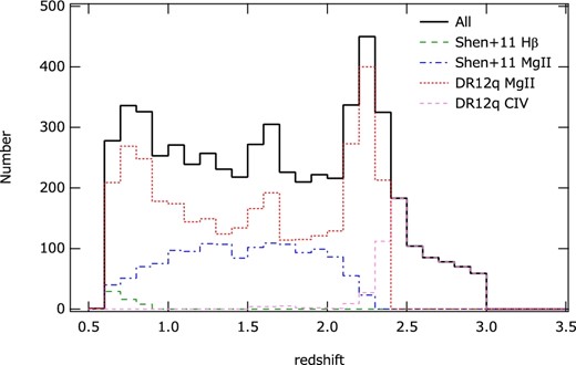
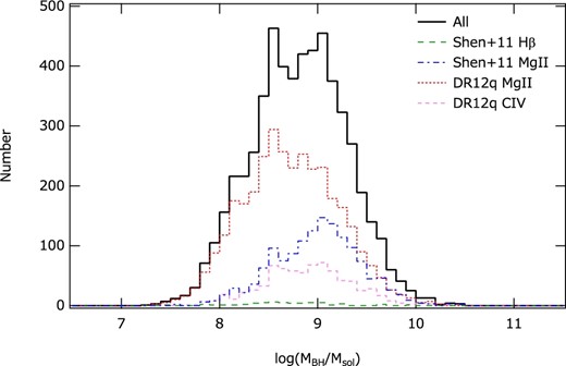
Figure 2 shows the mass vs redshift distribution of the AGNs that were selected according to the conditions described above and used in the cross-correlation analysis in this paper. Figures 3 and 4 show histograms of redshift and BH mass, respectively. We divided the redshift range into five groups as shown in figure 2, which we call z0, z1, z2, z3, and z4 for z = 0.6–1.0, 1.0–1.5, 1.5–2.0, 2.0–2.5, and 2.5–3.0, respectively. For each redshift group, except for z4, the BH mass range was divided into two groups, M8 and M9, such that each group has a similar number of AGNs rather than being divided at the same mass. This is because the effect of sample variance becomes dominant when the number of AGN samples is small and it is difficult to homogenize the samples among different mass groups by the division at constant mass for all the redshifts. The mass group was divided at log (MBH/M⊙) = 8.4, 8.8, 9.0, and 8.9 for z0, z1, z2, and z4 redshift groups, respectively, which allows us to make the statistical uncertainties even for both mass groups. The mass dependence of the z4 redshift group was not examined, since the number of samples in the z4 group is too small to do so.
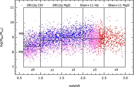
Distribution of redshift and BH mass of 5552 AGNs which are used in cross-correlation analysis using i-band detected galaxy samples. (Color online)
Distribution of BH mass for the samples shown in figure 2. (Color online)
Distribution of redshift for the samples shown in figure 2. (Color online)
Table 2 shows the number of AGN data sets which passed all the selection criteria described above for each data set. The i-band detected galaxy samples were used for cross-correlation analysis, and the four-band detected samples were used for deriving the color distribution and luminosity function of clustering galaxies, and they were also used to measure the dependence of cross-correlation length on galaxy luminosity. The redshift-matched samples were used for examining the BH mass dependence at each redshift.
Number of AGN samples used in the analysis for each data set.
| Redshift | i-band detected | Four-band detected | ||||
|---|---|---|---|---|---|---|
| group | All | z-matched* | All | z-matched | ||
| M8 + M9 | M8 | M9 | M8 + M9 | M8 | M9 | |
| z0† | 1194 | 482 | 482 | 1181 | 491 | 491 |
| z1† | 1216 | 506 | 506 | 1212 | 500 | 500 |
| z2† | 1235 | 534 | 534 | 1204 | 508 | 508 |
| z2‡ | 1202 | 503 | 503 | |||
| z3‡ | 1511 | 640 | 640 | 1385 | 581 | 581 |
| z4‡ | 396 | 363 | ||||
*Redshift-matched samples.
† M λ310-based samples for the four-band detected samples.
‡ M λ220-based samples for the four-band detected samples.
3 Analysis method
3.1 Cross-correlation length
The cross-correlation function between AGNs and galaxies was calculated using the method described in our previous papers (Shirasaki et al. 2011, 2016; Komiya et al. 2013). The analysis method is briefly described here.
In calculating n(rp), we masked the central 10″ around each AGN to avoid blending problems with the AGN. Around a bright source there is a region where the number density of the galaxy selected by the criteria described in subsection 2.2 is significantly reduced due to blending with the bright source and/or increase in the background noise level. That region needs to be counted as a dead region in calculating an effective area around AGNs.


| Parameter | Unit | Wavelength band | Coefficients |
|---|---|---|---|
| ϕ−18 | mag−1 Mpc−3 | Any | a 0 = −2.0, a1 = −0.175 |
| M * | mag | 150 nm | b 0 = −16.82, b1 = −2.437, b2 = 0.378 |
| M * | mag | 280 nm | b 0 = −17.57, b1 = −2.265, b2 = 0.351 |
| M * | mag | u΄ | b 0 = −18.40, b1 = −1.932, b2 = 0.294 |
| M * | mag | g΄ | b 0 = −20.38, b1 = −1.470, b2 = 0.250 |
| M * | mag | r΄ | b 0 = −21.60, b1 = −0.936, b2 = 0.157 |
| α | Any | c 0 = −1.2, c1 = 0.0 |
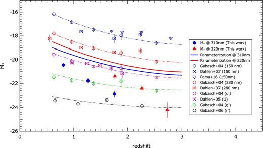
The root mean square (rms) of the difference between parameters from the literature and those calculated by the parametrization of equations (10)–(13) is 0.15 mag for log (ϕ−18), 0.28 mag for M*, and 0.14 mag for α. The error of log (ϕ−18) by 0.15 corresponds to a systematic error of r0 by ∼20% for γ = 1.8.
The error of M* significantly affects the luminosity densities at the bright end of M < M*, as the slope of the luminosity function becomes steeper there. Thus, comparison was made between the number densities at M < M* calculated using the parameters from the literature, ρlit, and those calculated with the above parametrization, ρpar. According to the comparison, the rms of the relative error (ρlit − ρpar)/ρpar is 0.36 for 40 sets of luminosity functions from the literature, which corresponds to an upper deviation of cross-correlation length of δr0 = 0.28 × r0, that is, 28% of the cross-correlation length, and a lower deviation of δr0 = 0.16 × r0, i.e., 16%, for γ = 1.8. When the comparison is made by extending to a lower luminosity side as M > −17, the rms of the relative error is 0.16 for 20 sets of luminosity functions of z < 1.5, which corresponds to upper and lower deviation of 10% and 8% for r0, respectively.
3.2 Color and absolute magnitude distributions for galaxies
To calculate the color and absolute magnitude for the same rest-frame bandpass at different redshifts, we performed spectral energy distribution (SED) fitting using the EAZY software developed by Brammer, van Dokkum, and Coppi (2008) and calculated color and magnitude at fixed bandpasses. For the redshift z0, z1, and z2 groups (z = 0.6–2.0), the color is defined as D1 = Mλ270 − Mλ380 and the absolute magnitude is Mλ310, where Mλ270, Mλ380, and Mλ310 represent absolute magnitudes at wavelengths 270, 380, and 310 nm, respectively. For the redshift z2, z3, and z4 groups (z = 1.5–3.0), the color is defined as D2 = Mλ165 − Mλ270 and the absolute magnitude is Mλ220, where Mλ165, Mλ270, and Mλ220 represent absolute magnitudes at wavelengths 165, 270, and 210 nm, respectively. For the redshift z2 group, we calculated the distributions for both definitions in order to compare between them.
Although EAZY can be used to estimate photometric redshift (photo-z), it was used here to interpolate the observed SEDs of all the sources assuming its redshift to be the same as the AGN redshift. This is because the photo-z is not well constrained at the redshifts explored in this work, as the structure around 400 nm, which is primarily used to determine the photo-z, is out of the observed passband. For this reason, photo-z was not used in our analysis and the clustering of galaxies was measured by stacking the galaxy distribution around AGNs and subtracting the constant density, which is a contribution from foreground/background galaxies, from the distribution.
4 Results
4.1 Cross-correlation function
First we present the cross-correlation functions derived by using the i-band detected galaxy samples for each redshift group. To also test for the dependence on galaxy luminosity, two galaxy samples were constructed with different threshold magnitudes. The threshold magnitudes were chosen to be |$M_{90\%}$| and |$M_{50\%}$|, where |$M_{90\%}$|(|$M_{50\%}$|) represents the absolute magnitude where the averaged detection efficiency estimated as described in subsection 3.1 is 90%(50%). The absolute magnitude is measured in the i-band observer frame as calculated with mi − DM, where mi is i-band apparent magnitude and DM is distance modulus for the AGN redshift. The values of |$M_{50\%}$| and |$M_{90\%}$| are summarized in the second and third columns of table 4.
Absolute magnitude thresholds |$M_{50\%}$|* and |$M_{90\%}$|† for each magnitude definition and each redshift group.
| Redshift | mi − DM | M λ310 | M λ220 | |||
|---|---|---|---|---|---|---|
| |$M_{50\%}$| | |$M_{90\%}$| | |$M_{50\%}$| | |$M_{90\%}$| | |$M_{50\%}$| | |$M_{90\%}$| | |
| (mag) | (mag) | (mag) | (mag) | (mag) | (mag) | |
| z0 | −17.61 | −18.40 | −17.82 | −18.80 | ||
| z1 | −18.77 | −19.49 | −19.12 | −20.01 | ||
| z2 | −19.65 | −20.34 | −20.17 | −21.06 | −19.97 | −20.85 |
| z3 | −20.40 | −21.09 | −20.74 | −21.55 | ||
| z4 | −20.93 | −21.62 | −21.36 | −22.20 | ||
*Absolute magnitudes where the detection efficiency is 50% for a given redshift group.
†Absolute magnitudes where the detection efficiency is 90% for a given redshift group.
Figure 8 shows the distributions of average number density of galaxies with absolute magnitude brighter than |$M_{50\%}$| for five redshift groups. The model functions of equa-tion (6) fitted to the observations are also plotted in the same figure. The corresponding projected cross-correlation functions calculated using equation (5) are shown in figure 9. The estimated fitting parameters are summarized in the upper parts of table 5 for each threshold magnitude.
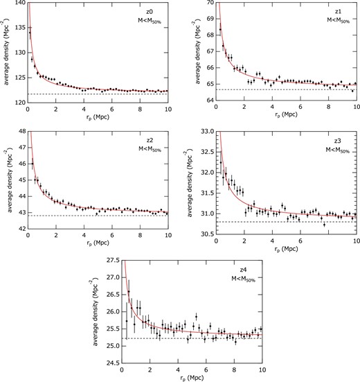
Radial distribution of galaxy surface density around AGNs for each redshift group. i-band detected galaxy samples with absolute magnitude brighter than |$M_{50\%}$| are used, where |$M_{50\%}$| represents the magnitude where detection efficiency is 50%. (Color online)
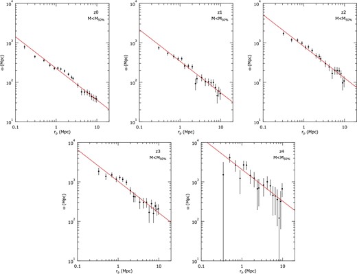
Projected cross-correlation functions derived from data shown in figure 8. Solid lines represent the power-law model fitted to the data. (Color online)
Fitting result of cross-correlation function.
| BH mass | Redshift | n AGN* | 〈log MBH/M⊙〉† | 〈z〉‡ | r 0 § | 〈nbg〉‖ | 〈ρ0〉♯ |
|---|---|---|---|---|---|---|---|
| log (MBH/M⊙) | h −1Mpc | Mpc−2 | 10−3 Mpc−3 | ||||
| |$M<M_{90\%}$| galaxy samples | |||||||
| 7.0–11.0 (M8 + M9) | 0.6–1.0 (z0) | 1194 | 8.45 | 0.78 | 6.66 ± 0.36 | 76.29 ± 0.03 | 11.2 |
| 7.0–11.0 (M8 + M9) | 1.0–1.5 (z1) | 1216 | 8.80 | 1.22 | 9.46 ± 0.69 | 42.53 ± 0.02 | 2.85 |
| 7.0–11.0 (M8 + M9) | 1.5–2.0 (z2) | 1235 | 8.94 | 1.74 | 16.05 ± 1.09 | 28.73 ± 0.02 | 0.886 |
| 7.0–11.0 (M8 + M9) | 2.0–2.5 (z3) | 1511 | 8.96 | 2.25 | 19.07 ± 2.06 | 20.67 ± 0.01 | 0.299 |
| 7.0–11.0 | 2.5–3.0 (z4) | 396 | 8.90 | 2.72 | 35.24 ± 6.41 | 16.89 ± 0.02 | 0.0968 |
| |$M<M_{50\%}$| galaxy samples | |||||||
| 7.0–11.0 (M8 + M9) | 0.6–1.0 (z0) | 1194 | 8.45 | 0.78 | 6.89 ± 0.36 | 121.73 ± 0.04 | 15.5 |
| 7.0–11.0 (M8 + M9) | 1.0–1.5 (z1) | 1216 | 8.80 | 1.22 | 8.67 ± 0.58 | 64.67 ± 0.03 | 4.92 |
| 7.0–11.0 (M8 + M9) | 1.5–2.0 (z2) | 1235 | 8.94 | 1.74 | 14.02 ± 0.77 | 42.82 ± 0.02 | 1.85 |
| 7.0–11.0 (M8 + M9) | 2.0–2.5 (z3) | 1511 | 8.96 | 2.25 | 16.08 ± 1.21 | 30.80 ± 0.02 | 0.777 |
| 7.0–11.0 | 2.5–3.0 (z4) | 396 | 8.90 | 2.72 | 23.58 ± 3.62 | 25.22 ± 0.03 | 0.332 |
| Redshift-matched AGN samples and |$M<M_{90\%}$| galaxy samples | |||||||
| 7.0–8.4 (M8) | 0.6–1.0 (z0) | 482 | 8.08 | 0.77 | 6.00 ± 0.61 | 75.42 ± 0.04 | 11.4 |
| 8.4–11.0 (M9) | 0.6–1.0 (z0) | 482 | 8.76 | 0.77 | 6.98 ± 0.55 | 76.44 ± 0.04 | 11.4 |
| 7.0–8.8 (M8) | 1.0–1.5 (z1) | 506 | 8.45 | 1.22 | 9.07 ± 1.08 | 42.03 ± 0.03 | 2.85 |
| 8.8–11.0 (M9) | 1.0–1.5 (z1) | 506 | 9.14 | 1.22 | 9.07 ± 1.14 | 43.05 ± 0.03 | 2.86 |
| 7.0–9.0 (M8) | 1.5–2.0 (z2) | 534 | 8.61 | 1.74 | 14.91 ± 1.75 | 28.67 ± 0.03 | 0.890 |
| 9.0–11.0 (M9) | 1.5–2.0 (z2) | 534 | 9.33 | 1.74 | 16.89 ± 1.65 | 28.95 ± 0.03 | 0.887 |
| 7.0–8.9 (M8) | 2.0–2.5 (z3) | 640 | 8.56 | 2.25 | 19.47 ± 3.10 | 20.75 ± 0.02 | 0.299 |
| 8.9–11.0 (M9) | 2.0–2.5 (z3) | 640 | 9.29 | 2.25 | 22.04 ± 2.78 | 20.61 ± 0.02 | 0.300 |
*Number of AGN data sets.
†Average of logarithm of BH mass.
‡Average redshift.
§Cross-correlation length and its error.
‖Average of projected number density of background galaxies.
♯Average of the averaged number density of galaxies at the AGN redshift.
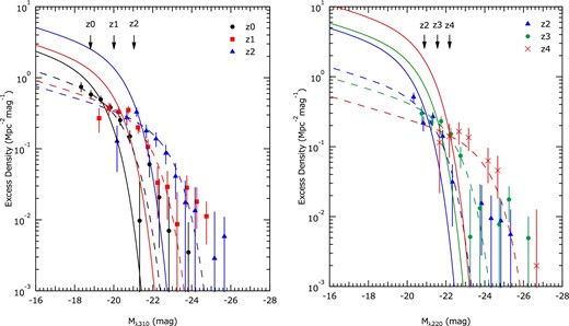
The cross-correlation lengths are plotted as a function of redshift in figure 10 for each threshold sample. The result shows that the cross-correlation length increases as the redshift increases, and is also larger for more luminous galaxy samples. Therefore, for examining the BH mass dependence, it is important to match the distribution of redshift and galaxy luminosity for different BH mass gruops.
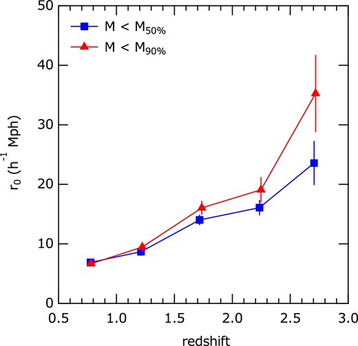
Cross-correlation length as a function of redshift. Squares and triangles represent the cross-correlation length derived using galaxies brighter than |$M_{50\%}$| and |$M_{90\%}$|, respectively, where |$M_{50\%}$| (|$M_{90\%}$|) represents the magnitude where detection efficiency is 50% (90%). (Color online)
To reduce the effect of redshift dependence in the comparisons between the different BH mass groups, we constructed redshift-matched samples for each redshift group. The redshift-matched samples were constructed by selecting the same number of AGN data sets for each Δz = 0.02 bin. The projected cross-correlation functions calculated for the redshift-matched samples are shown in figure 11 for four redshift groups z0, z1, z2, and z3. The mass dependence for the z4 group was not examined due to poor statistics. In this figure, the circles represent lower BH mass groups (M8) and the squares represent higher BH mass groups (M9). Galaxy samples brighter than |$M_{90\%}$| were used. The estimated fitting parameters are summarized in the bottom part of table 5.
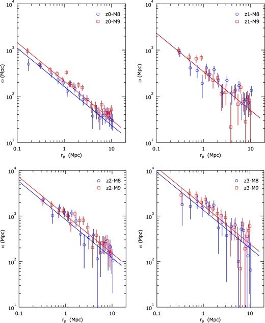
Comparisons of projected cross-correlation functions derived for mass groups of M8 (circles) and M9 (squares). Each panel represents the result for redshifts z0, z1, z2, and z3. Redshift-matched AGN samples and galaxy samples brighter than |$M_{90\%}$| are used. Solid lines represent the power-law model fitted to the data points. (Color online)
The cross-correlation lengths are plotted as a function of BH mass in figure 12. From these results, no significant difference is seen between the two mass groups.
Cross-correlation lengths plotted as a function of average BH mass obtained for data shown in figure 11 (blue solid markers). Note that the galaxy sample for these data sets are dominated by blue galaxies. The result obtained by Shirasaki et al. (2016), for which galaxy samples are dominated by red galaxies contrary to the current data set, is shown with crosses. The result obtained using the data selected by color to construct a data set comparable with the result of Shirasaki et al. (2016) is shown with open circles. (Color online)
For comparison with the previous results (Shirasaki et al. 2016) derived using UKIDSS and SDSS data for galaxy samples, the results obtained for red galaxy samples (D1 ≥ 1.4) as described in the next subsection are also plotted. In their work, Shirasaki et al. (2016) calculated cross-correlation functions between AGNs and galaxies, which were mostly red galaxies, at redshifts <1.0, and obtained the result that the cross-correlation length depends on BH mass but does not depend on redshift. Our current result at higher redshifts indicates its strong dependence on redshift and not on BH mass. The different behavior partly comes from the difference in the properties of galaxy samples; that is, the galaxy samples in the previous work are dominated by red-type galaxies and mostly dimmer than characteristic luminosity L* of the Schechter function, while those in the current work are dominated by blue-type galaxies and mostly consist of galaxies brighter than L* at higher redshifts. As shown in the following subsection, the clustering of galaxies significantly increases above L*, which introduces redshift dependence to the cross-correlation length.
4.2 Galaxy luminosity-dependence of cross-correlation length
As larger clustering was indicated for more luminous galaxies as shown in figure 10, we calculated cross-correlation lengths for flux-limited samples derived from the four-band detected samples to examine the dependence on the luminosity of galaxies more closely. To calculate the absolute magnitude for the same rest-frame bandpass at different redshifts, we performed SED fitting using the EAZY software developed by Brammer, van Dokkum, and Coppi (2008) and calculated the magnitude at a fixed bandpass. The observed magnitudes at g, r, i, z, and y bands are used in the SED fitting. The flux-limited galaxy samples were constructed based on absolute magnitude Mλ310 for z0, z1, and z2, and Mλ220 for z2, z3 and z4, where Mλ310 and Mλ220 represents the absolute magnitude at wavelength 310 nm and 220 nm, respectively.
Cross-correlation length as a function of average absolute magnitude of galaxies measured in Mλ310 or Mλ220. The cross-correlation lengths were calculated using the galaxy samples which are brighter than given threshold magnitudes. Dotted lines represent functions of equation (20) fitted to the data points. (Color online)
Cross-correlation length as a function of M* − 〈Mλ310〉 or M* − 〈Mλ220〉. 〈Mλ310〉 and 〈Mλ220〉 are the average absolute magnitudes of galaxies measured at rest-frame wavelengths of 310 nm and 220 nm, respectively, and the cross-correlation lengths were calculated by using the galaxy samples which are brighter than the threshold magnitude. Dotted lines represent functions of equation (20) fitted to the data points. (Color online)
From these figures, it is apparent that the cross-correlation length rapidly increases at magnitudes brighter than M*, and it also increases with increasing redshift when compared for the same M* − M. r0, min corresponds to the cross-correlation length calculated for the whole galaxy samples of each redshift group. Due to the difference in the detection threshold of galaxy luminosity, the average luminosity for all the galaxy samples is larger for the higher redshift groups than for the lower ones. Thus the difference of r0, min is due to the difference in galaxy luminosity as well as the difference in redshift.
4.3 Color distributions of galaxies around AGNs
Color distributions of galaxies around AGNs were derived by the subtraction method described in subsection 3.2, and the results are shown in figure 15 for color parameter D1 at z0 to z2 and in figure 16 for D2 at z2 to z4. Redshift-matched AGN samples were used for this analysis. The galaxy samples used are the four-band detected samples, and the threshold magnitude for the galaxy was chosen to be |$M_{50\%}$|, which is an absolute magnitude where the average detection efficiency is 50%. The measured values of |$M_{50\%}$| are summarized in the fourth and sixth columns of table 4.
Color (D1) distributions derived for redshift-matched AGNs and |$< M_{50\%}$| galaxy samples calculated as shown in equation (17). The panels in the left-hand column are the distributions for combined mass groups (M8 + M9), and on the right of each row are the distributions for individual mass groups of M8 and M9. The top three panels are those for redshift z0, and the middle and bottom panels are for z1 and z2, respectively. The solid lines represent the results of double Gaussian fitting. The dashed vertical lines represent the boundary-defining blue and red galaxies in this paper. (Color online)
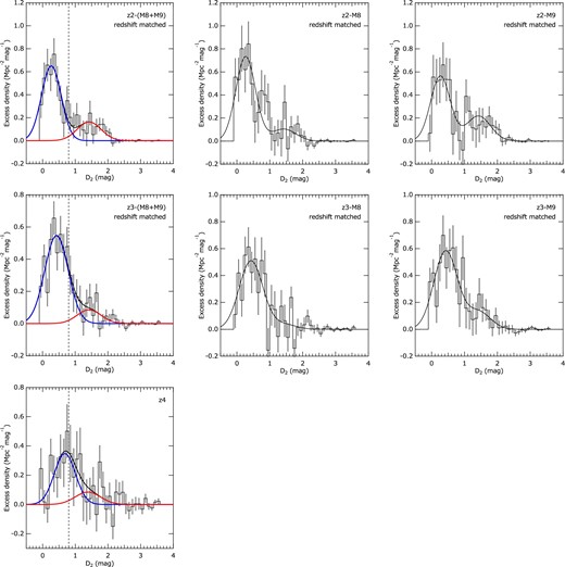
Color (D2) distributions derived for redshift-matched AGNs and |$<\! M_{50\%}$| galaxy samples calculated as shown in equation (17). The panels in the left-hand column are the distributions for combined mass groups (M8 + M9), and the two panels on the right of each row are the distributions for individual mass groups of M8 and M9. The top three panels are those for redshift z2, and the middle and bottom panels are for z3 and z4, respectively. The solid lines represent the results of double Gaussian fitting. The dashed vertical lines represent the boundary-defining blue and red galaxies in this paper. (Color online)
The panels in the left-hand column in the figures show the excess color density of D1 or D2 distributions for combined M8 + M9 groups, and they are placed in increasing order of their redshifts from top to bottom. The two panels on the right-hand side of each row are those for M8 and M9 groups at the corresponding redshift, respectively. In the case of the z4 group, only the distribution of the whole mass group is shown, as the number of samples is too small to split the sample into two mass groups for the analysis of mass dependence. D1 is defined as a difference between magnitudes at rest-frame wavelengths of 270 nm and 380 nm for redshift groups z0, z1, and z2, and D2 is a color between magnitudes at 165 nm and 270 nm for redshift groups z2, z3, and z4. The magnitudes were calculated by performing SED fitting using the EAZY software (Brammer et al. 2008) as described in subsection 3.2.
The color distributions were fitted with a double Gaussian model in which the two Gaussian functions correspond to red (smaller D1) and blue (larger D1) galaxy types. The fitted model functions are plotted in the same figures. As can be seen from the color distributions in figures 15 and 16, blue galaxies dominate the clustered component in our galaxy samples.
In the fit to the D1 distribution for the z2 (M8 + M9) group shown in figure 15, the Gaussian parameters for each component were not well constrained. This is partly because there is a tendency for the distribution of the blue component to shift to the redder side as the redshift increases, and the components overlap in higher fractions for that group. Thus we fixed the Gaussian parameters of the red component to those obtained for the z1 (M8 + M9) group. In the cases of z3 and z4 shown in figure 16, the red component is barely visible, thus the Gaussian parameters for the red component were fixed to those obtained for D2 distribution of z2 (M8 + M9).
The fitting for the M8 and M9 samples was performed by fixing the Gaussian parameters to those obtained for the combined M8 + M9 samples except for the z0 group. In the case of z0, the peak positions of the blue component are slightly different between the M8 and M9 groups. Thus, the Gaussian parameters for the blue component were derived independently. Those fitting parameters are summarized in table 6.
Fitting result for color distribution.*
| Redshift | BH mass | n AGN | μblue† | σblue‡ | μred§ | σred‖ | f blue ♯ |
|---|---|---|---|---|---|---|---|
| log (MBH/M⊙) | |||||||
| D 1, combined mass group | |||||||
| 0.6–1.0 (z0) | 7.0–11.0 (M8 + M9) | 982 | 0.55 ± 0.05 | 0.38 ± 0.05 | 1.59 ± 0.19 | 0.56 ± 0.08 | 0.71 ± 0.09 |
| 1.0–1.5 (z1) | 7.0–11.0 (M8 + M9) | 1000 | 0.73 ± 0.02 | 0.21 ± 0.02 | 1.86 ± 0.06 | 0.35 ± 0.04 | 0.78 ± 0.03 |
| 1.5–2.0 (z2) | 7.0–11.0 (M8 + M9) | 1016 | 0.88 ± 0.04 | 0.36 ± 0.04 | 1.86 | 0.35 | 0.70 ± 0.04 |
| D 2, combined mass group | |||||||
| 1.5–2.0 (z2) | 7.0–11.0 (M8 + M9) | 1006 | 0.27 ± 0.04 | 0.30 ± 0.05 | 1.42 ± 0.13 | 0.37 ± 0.08 | 0.76 ± 0.06 |
| 2.0–2.5 (z3) | 7.0–11.0 (M8 + M9) | 1162 | 0.43 ± 0.04 | 0.36 ± 0.04 | 1.42 | 0.37 | 0.86 ± 0.05 |
| 2.5–3.0 (z4) | 7.0–11.0 | 396 | 0.69 ± 0.10 | 0.33 ± 0.09 | 1.42 | 0.37 | 0.79 ± 0.17 |
| D 1, individual mass group | |||||||
| 0.6–1.0 (z0) | 7.0–8.4 (M8) | 491 | 0.45 ± 0.04 | 0.35 ± 0.04 | 1.59 | 0.56 | 0.76 ± 0.03 |
| 8.4–11.0 (M9) | 491 | 0.71 ± 0.04 | 0.32 ± 0.04 | 1.59 | 0.56 | 0.64 ± 0.04 | |
| 1.0–1.5 (z1) | 7.0–8.8 (M8) | 500 | 0.73 | 0.21 | 1.86 | 0.35 | 0.78 ± 0.04 |
| 8.8–11.0 (M9) | 500 | 0.73 | 0.21 | 1.86 | 0.35 | 0.79 ± 0.03 | |
| 1.5–2.0 (z2) | 7.0–9.0 (M8) | 508 | 0.88 | 0.36 | 1.86 | 0.35 | 0.80 ± 0.05 |
| 9.0–11.0 (M9) | 508 | 0.88 | 0.36 | 1.86 | 0.35 | 0.61 ± 0.05 | |
| D 2, individual mass group | |||||||
| 1.5–2.0 (z2) | 7.0–9.0 (M8) | 503 | 0.27 | 0.30 | 1.42 | 0.37 | 0.85 ± 0.05 |
| 9.0–11.0 (M9) | 503 | 0.27 | 0.30 | 1.42 | 0.37 | 0.68 ± 0.05 | |
| 2.0–2.5 (z3) | 7.0–8.9 (M8) | 581 | 0.43 | 0.36 | 1.42 | 0.37 | 0.93 ± 0.07 |
| 8.9–11.0 (M9) | 581 | 0.43 | 0.36 | 1.42 | 0.37 | 0.81 ± 0.05 | |
*Redshift-matched AGN data sets and four-band (griz) detected galaxies brighter than |$M_{50\%}$| were used.
†Mean of the D1 or D2 distribution for the blue component.
‡Standard deviation of the D1 or D2 distribution for the blue component.
§Mean of the D1 or D2 distribution for the red component.
‖Standard deviation of the D1 or D2 distribution for the red component.
♯Fraction of blue component.
The fractions of the blue galaxy for the combined groups made up of the M8 and M9 mass groups are around 0.7–1.0, and there is a marginal indication that the blue fraction increases at higher redshifts. Care needs to be taken in the comparison of the different redshifts by noting the difference in the galaxy samples. The galaxy samples at higher redshift are biased to more luminous galaxies, and it is also expected that the fraction of red galaxies increases along with the increase in luminosity as observed in the color–magnitude diagrams of the local galaxies. Thus the observed redshift dependence of the blue fraction is biased to the red component at higher redshift, and it is expected that the increase in the blue fraction is more or less enhanced if the bias is corrected.
As already mentioned above, the peak position of the blue galaxy is found to shift to the redder side as redshift increases. We also found that the peak position shifts to the redder side for brighter galaxies of the same redshift, so the shift of the peak position to the redder side at higher redshift is partly due to the dependence of the color on the absolute magnitude of the galaxy.
The obtained blue galaxy fractions are plotted in figure 17 as a function of BH mass for each redshift group. A decreasing trend of blue fraction with BH mass is found for all redshifts except for z1. The result of z1 might have suffered from the sample variance. This can be tested by adding more samples from the upcoming HSC-SSP survey.

In the previous work of Shirasaki et al. (2016) that used SDSS and UKIDSS for galaxy samples, the blue galaxy fraction was less than ∼0.2 at redshift group z0 of this work, as the galaxy sample was strongly biased to red-type galaxies. In that work they also obtained the result that red galaxies more luminous than MIR = −20 were strongly clustered around AGNs of MBH > 108.2 M⊙. To test the consistency with the previous result on the cross-correlation with red galaxies, we calculated the cross-correlation lengths for red galaxies in the z0-M8 and z0-M9 groups separately.
We extracted red galaxies defined as D1 ≥ 1.4, and restricted their brightness to |$M_{\lambda 310} < M_{90\%} (=\! -18.8)$|. To calculate the cross-correlation function, we need to know the average number density of these galaxy types at the corresponding redshift, |$\bar{\rho }_{0, \rm red}$|. It was estimated as |$\bar{\rho }_{0} (1-f_{\rm blue})$| using the blue fraction determined for z0-M8 group. Then we obtained the cross-correlation lengths for red galaxy samples as r0, red = 6.35 ± 1.22 for z0-M8, and r0, red = 8.73 ± 1.02 for z0-M9. The values of r0, red are plotted in figure 12 and compared with the previous work. They are consistent with each other.
4.4 Luminosity functions of galaxies around AGNs
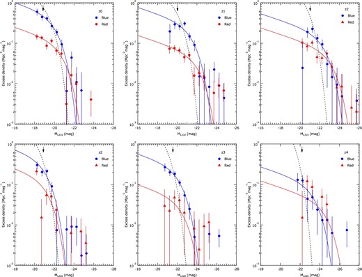
Next we examined the absolute magnitude distributions of the galaxy clustered around AGNs. The left(right)-hand panel of figure 18 shows the distributions of Mλ310 (Mλ220) for z0, z1, and z2 (z2, z3, and z4) redshift groups. The excess densities were calculated as in equation (18) and corrected for their detection efficiencies calculated as described in subsection 3.1. They are plotted for Mλ310, |$M_{\lambda 220} < M_{50\%}$|.
Absolute magnitude distributions of galaxies around AGNs calculated as in equation (18). Detection efficiencies were corrected and plotted for |$M<M_{50\%}$|. The left-hand panel shows the distributions measured in Mλ310 for z0, z1, and z2 groups. The right-hand panel shows the distributions measured in Mλ220 for z2, z3, and z4 groups. The solid lines represent the luminosity function calculated by the parametrization used in this work and scaled by a factor calculated from the cross-correlation length obtained for |$M_{50\%}$| galaxy samples. The scaling factor was calculated as in equa-tion (21). The dashed lines represent Schechter functions fitted to the data points. The arrows at the top of the panels indicate the 90% detection limit. (Color online)
To test if the overdensity can be explained by the uncertainty of the M* parameter used in the parametrization of luminosity function model, we measured the M* parameters for the observed magnitude distributions by fitting the Schechter function to them and compared them with the values given by the parametrization. In the fitting α was fixed to −1.2. The results are summarized in table 7 and compared in figure 19 with the parametrization (thick solid lines) and literature values (open markers). The obtained M* are typically smaller (i.e., brighter) than M* given by the parameterization by >1 mag, well exceeding the uncertainty of M*, 0.28 mag, expected for the parametrization. Thus it is unlikely that the overdensity is attributable only to the uncertainty of the assumed luminosity function.
Comparisons of M* parameters measured for clustering galaxies around AGNs and those calculated from the parametrization.
| Redshift | Average | Wavelength | M *(clust)† | M *(param)‡ | |${\Delta }$| M * § |
|---|---|---|---|---|---|
| group | redshift | (nm) | (mag) | (mag) | (mag) |
| z0 | 0.81 | 310 | −20.4 ± 0.2 | −19.3 | 1.1 |
| z1 | 1.26 | 310 | −21.8 ± 0.2 | −20.0 | 1.8 |
| z2 | 1.75 | 310 | −22.9 ± 0.3 | −20.6 | 2.3 |
| z2 | 1.76 | 220 | −21.4 ± 0.2 | −20.3 | 1.1 |
| z3 | 2.26 | 220 | −22.4 ± 0.3 | −20.7 | 1.7 |
| z4 | 2.74 | 220 | −24.2 ± 0.7 | −21.0 | 3.2 |
† M * parameters measured for clustering galaxies around AGN.
‡ M * parameters calculated from the parametrization as described in subsection 3.1.
§ M *(param) − M*(clust).
To investigate the galaxy type that contributes to the overdensity at the bright end, we derived the magnitude distributions for blue and red galaxies separately. They were classified at D1 = 1.4 or D2 = 0.8. Figure 20 shows the comparisons between the magnitude distributions for blue and red galaxies. Both galaxy types contribute to the overdensity.
Comparison of M* parameters measured for clustering galaxies around AGNs (filled circles and filled triangles) and those calculated from the parametrization (thick solid lines). M* values derived in literature (Gabasch et al. 2004, 2006; Dahlen et al. 2005, 2007; Parsa et al. 2016) are also plotted. (Color online)
Absolute magnitude distributions for blue and red galaxies calculated as in equation (18). The dashed lines represent the luminosity function calculated by the parametrization used in this work and scaled by a factor calculated from the cross-correlation length. The scaling factor was calculated as in equation (21). The solid lines represent Schechter functions fitted to the data points. The arrows at the top of the panels indicate the 90% detection limit. (Color online)
M * parameters measured for the distributions are summarized in table 8 and plotted in figure 21. The obtained M* parameters for red galaxies are systematically brighter than those for blue galaxies by more than two sigma at redshift z0, z1, and z2 for measurements at 310 nm. No statistically significant difference is found for the values for z2, z3, and z4 measured at 220 nm, which is mostly due to poor statistics and lower resolution of D2 parameters on the deconvolution of the two components.
Comparison of M* parameters measured for blue and red galaxies. These are obtained by fitting Schechter functions to the data points in figure 20.
Comparisons of M* parameters measured for clustering galaxies around AGNs for blue and red galaxy types.
| Redshift | Wavelength | M *(blue) | M *(red) |
|---|---|---|---|
| (nm) | (mag) | (mag) | |
| z0 | 310 | −20.29 ± 0.18 | −20.95 ± 0.25 |
| z1 | 310 | −21.66 ± 0.23 | −22.29 ± 0.37 |
| z2 | 310 | −22.60 ± 0.35 | −23.36 ± 0.36 |
| z2 | 220 | −21.28 ± 0.22 | −21.42 ± 0.53 |
| z3 | 220 | −22.38 ± 0.20 | −22.67 ± 1.13 |
| z4 | 220 | −23.57 ± 0.53 | −24.78 ± 1.43 |
We also investigated whether there is a difference in the luminosity functions of clustering galaxies for lower and higher BH mass groups. Figure 22 shows the comparisons between the magnitude distributions for the M8 and M9 mass groups, and M* parameters measured for them are summarized in table 9 and plotted in figure 23.
Absolute magnitude distributions for M8 and M9 mass groups. The dashed lines represent luminosity function calculated by the parametrization used in this work and scaled by a factor calculated from the cross-correlation length. The scaling factor was calculated as in equation (21). The solid lines represent Schechter functions fitted to the data points. The arrows at the top of the panels indicates the 90% detection limit. (Color online)
Comparison of M* parameters measured for M8 and M9 mass groups. These are obtained by fitting Schechter functions to the data points in figure 22.
Comparisons of M* parameters measured for clustering galaxies around AGNs of M8 and M9 groups.
| Redshift | Wavelength | M *(M8) | M *(M9) |
|---|---|---|---|
| (nm) | (mag) | (mag) | |
| z0 | 310 | −20.29 ± 0.24 | −20.83 ± 0.21 |
| z1 | 310 | −21.36 ± 0.40 | −22.12 ± 0.32 |
| z2 | 310 | −22.93 ± 0.34 | −23.06 ± 0.52 |
| z2 | 220 | −21.50 ± 0.32 | −21.22 ± 0.35 |
| z3 | 220 | −22.58 ± 0.41 | −22.44 ± 0.28 |
The obtained M* parameters for the M9 group are systematically brighter than those for the M8 group by more than two sigma at redshifts z0 and z1. No statistically significant difference is found for the values at redshift z2 (for both 310 nm and 220 nm) and z3. The results may indicate the enhancement of bright galaxies around AGNs with higher BH mass ( > 108.5 M⊙) at redshift <1.5, while at redshift ≥1.5 the luminosity function of a galaxy is similar around AGNs with BH mass of ≥ 108 M⊙.
4.5 AGN linear bias and dark matter halo mass hosting AGNs
The AGN–galaxy cross-correlation functions can be used to measure the linear bias of AGN distribution then to estimate the average mass of dark matter halos hosting the AGNs. Using the relation between the halo mass and its bias obtained by numerical simulation, we can estimate the halo mass by assuming that the AGNs are located in halos with a similar bias.
To derive the linear bias of AGNs from the AGN–galaxy cross-correlation function, we should know also about the auto-correlation function of galaxies. It is not, however, determined only from the data set used in this work. Thus, we assume that auto-correlation functions measured by Zehavi et al. (2011), which were derived by using the SDSS galaxies at redshifts <0.25, does not change up to redshift =3. Since the galaxy auto-correlation functions measured at higher redshifts (e.g., Ishikawa et al. 2015) are almost the same as those measured by Zehavi et al. (2011), it can be a good approximation.
The primary cause of the larger clustering of our galaxy samples is due to the evolution of, i.e., decrease in, the M* parameter in the luminosity function at neighbors of AGNs, as shown in the subsection 4.4. To reduce the effect of the M* evolution and derive ξAG for <M* galaxies, we calculated the cross-correlation lengths from the magnitude distributions of the clustering galaxies, nfit(M), which were obtained by fitting the Schecher function to the observation in estimating M* for the measured magnitude distributions. The parameter α of the Schecher function was fixed to −1.2. The magnitude distributions, nfit(M), are shown in figure 18 as dashed lines.
AGN linear bias and the dark matter halo mass.
| Redshift | |$r^{\prime }_{\rm AG}$|* | r AA † | γAA‡ | b AGN § | log (Mh/M⊙)‖ |
|---|---|---|---|---|---|
| (h−1 Mpc) | (h−1 Mpc) | ||||
| z0 | 5.5 ± 0.3 | 6.4 ± 0.6 | 1.77 | 2.06 ± 0.17 | 13.0|$^{+0.1}_{-0.2}$| |
| z1 | 5.3 ± 0.3 | 6.3 ± 0.7 | 1.79 | 2.49 ± 0.26 | 12.9 ± 0.2 |
| z2 | 5.4 ± 0.4 | 6.1 ± 0.9 | 1.76 | 2.90 ± 0.37 | 12.6 ± 0.2 |
| z3 | 6.9|$^{+0.6}_{-0.7}$| | 11.2 ± 2.0 | 1.83 | 6.03|$^{+0.97}_{-1.01}$| | 13.3|$^{+0.2}_{-0.3}$| |
| z4 | 5.5|$^{+1.0}_{-1.1}$| | 6.8|$^{+2.6}_{-2.4}$| | 1.80 | 4.29|$^{+1.37}_{-1.49}$| | 12.5|$^{+0.4}_{-0.8}$| |
*AGN–galaxy cross-correlation length for >M* galaxies around AGNs.
†AGN auto-correlation length.
‡Power-law index of AGN auto-correlation function.
§AGN bias.
‖Average mass of the dark matter halos hosting the AGNs.
Summary of the names of the AGN data set groups and of the parameters frequently refereed to in the text.
| Group or parameter name | Description |
|---|---|
| z0, z1, z2, z3 | Names of the redshift group defined in figure 2. |
| M8, M9 | Names of the BH mass group defined in figure 2. |
| M *,† | Characteristic absolute magnitude of the Schechter function as defined in equation (9). |
| |$M_{50\%}$|, |$M_{90\%}$| | Absolute magnitudes where the detection efficiency is 50% and 90% for a given redshift group. |
| M λ310, Mλ220 | Absolute magnitudes at wavelengths of 310 nm and 220 nm in the source frame. |
| D 1, D2 | Color parameters defined for redshifts 0.6–2.0 and 1.5–3.0; see subsection 3.2 for their definitions. |
| f blue | Blue galaxy fraction. |
| ρ0‡ | Average number density of galaxies which are brighter than the threshold magnitude and can be detected at the redshift of AGN. |
| ξ(r), ω(rp) | Correlation function and projected correlation function. |
| r 0(=rAG), γ | Cross-correlation length and power law index of the AGN–galaxy cross-correlation function as defined in equation (3). |
| r AA, rGG | Auto-correlation lengths of AGNs and galaxies. |
| M BH | Black hole mass. |
| M h | Dark matter halo mass. |
| b AGN | AGN bias. |
†Where necessary, this parameter is distinguished as M*(param) or M*(clust) for describing the M* given by the parametrization discussed in subsection 3.1 and that measured from this observational data.
‡This parameter is calculated integrating the product of luminosity function and detection efficiency function as given in equation (16). The luminosity function is given by the parametrization as described in subsection 3.1, and the detection efficiency function is measured for each AGN data set as described in subsection 3.1.
The obtained AGN biases, bAGN, are plotted as a function of redshift, using solid circles, in figure 24. The AGN biases obtained in the literature (Hickox et al. 2009; Krumpe et al. 2012; Ross et al. 2009; Croom et al. 2005) are also shown for comparison. In the figure, the bias expected for three halo masses, log (Mh/M⊙) = 12.0, 12.5, and 13.0, is plotted with dashed lines. The obtained bias at redshift <2.0 is consistent with those obtained in other studies, and hosted by dark matter halos with average mass in the range of 1012.5–1013.0 M⊙. The large scatters of our results at >2.0 is mostly due to the dominance of <M* galaxies in our samples, which introduce large error in the correction of rAG to |$r^{\prime }_{\rm AG}$|.
Evolution of the AGN bias. Solid circles are the result obtained in this work by assuming no evolution in galaxy auto-correlation function for z = 0–3 and correcting the AGN–galaxy cross-correlation for the M* evolution around AGNs. The dashed line represents the bias of the dark matter halos calculated using the relation of equation (33) (Sheth et al. 2001) for log (Mh/M⊙) = 13.0, 12.5, and 12.0 from top to bottom. As a comparison, results obtained in literature are also plotted as labeled in the annotation. The results from Hickox et al. (2009); Krumpe et al. (2012) are derived from the AGN–galaxy cross-correlation, and those from Ross et al. (2009); Croom et al. (2005) are from AGN auto-correlation. (Color online)
5 Discussion and conclusion
The dependence of AGN–galaxy cross-correlation on redshift, galaxy luminosity, and BH mass was examined. The galaxy samples used in this analysis are dominated with blue-type galaxies, and the fraction of blue-type galaxies is more than 70%. No significant dependence on the BH mass was found for the cross-correlation length derived using whole galaxy samples. Considering that the error of BH mass estimation can be as large as 0.4 dex, as explained in subsection 2.1, the BH mass dependence can be diluted when compared in a mass range as small as the uncertainty of BH mass, which is ∼1 dex in our sample for each redshift group. To investigate the relation between BH mass and the host halo mass, it is required to test the mass dependence for a wider BH mass range using a more accurate mass estimator.
However, we obtained an indication that cross-correlation with red galaxies is larger for larger BH mass at the lowest redshift group, as shown in figure 12, which is consistent with previous studies (Komiya et al. 2013; Shirasaki et al. 2016) in which galaxy samples are strongly biased to a red type. The BH mass dependence for the cross-correlation of red galaxies and AGN obtained in this work is marginal, but it is encouraging to see that we obtained a positive correlation for different data sets.
What does this different BH mass dependence for red and blue galaxies mean? It is unrealistic to think about a direct and physical connection between BHs and galaxies separated by more than 1 Mpc. One possible idea to explain such a dependence is the interaction at a scale of halos (i.e., groups/clusters interaction), which causes concurrent encounters of constituent galaxies and induces ram pressure stripping of interstellar medium (ISM) and/or hot gas in galaxy halos, and also brings about galaxy mergers and subsequent star formation (Mihos 2004). This may result in the increase in the number density of red galaxies, and also the M* evolution. Since those encounters happen to only a part of galaxies, the number density of the dominant component of blue galaxies is almost unchanged.
The redshift dependence of the cross-correlation length was found as shown in figure 10, and it turned out to be most primarily due to the luminosity dependence of galaxy clustering and its redshift evolution. The luminosity dependence of galaxy clustering has been reported in literature (e.g., Zehavi et al. 2011; Ishikawa et al. 2015). Zehavi et al. (2011) and Ishikawa et al. (2015) measured auto-correlation lengths for galaxy samples divided by their luminosity, and obtained r0 = 4–5 h−1 Mpc for the lower luminosity groups and ∼10 h−1 Mpc for the most luminous group. Our measurements indicate larger clustering than those found in the literature, which will be discussed in a later part of this section.
The observed luminosity dependence can be explained as a result of a shift in the M* parameter by >1 mag to the luminous side as shown in subsection 4.3. This indicates that the star-formation activity is relatively larger around AGNs in our sample compared to those in a general field at the same redshift.
The fraction of red galaxies in the environment can be a measure of the degree of progress on galaxy formation and evolution in that system. The fraction may depend on the frequency of events that trigger the star-formation activity, such as major/minor merger and/or interaction with a nearby galaxy, and also the time scale of the star-formation quenching. If the frequency of the triggering event is higher and the time scale of the quenching is shorter, the galaxy formation and evolution rapidly proceed and the red galaxy fraction is increased in such an environment. In such an environment, it is also expected that the SMBHs rapidly increase their mass through the mass accretion caused by a similar kind of event which triggers the star formation in the galaxies around it.
As blue galaxies are dominant, the transformation of only a small fraction of blue galaxies to red galaxies can significantly affect the clustering strength of the red galaxies. This may be an explanation for the clustering of whole galaxies (both blue and red galaxies) almost being independent of the BH mass, while the clustering of red galaxies depend on the BH mass as reported in (Komiya et al. 2013; Shirasaki et al. 2016).
The peak position of the color distributions for blue galaxies was measured as shifting to the redder side as the redshift increased. This is at least partly due to the the luminosity dependence of the peak position. This result may indicate that the luminous star-forming galaxies at these redshifts are reddened by dust or by some other mechanism.
AGN bias was calculated from the AGN–galaxy cross-correlation length. As described above we found that the galaxies around AGNs of our samples have significantly larger clustering due to the evolution of M* of the luminosity function. The galaxy auto-correlation function, which was required to derive the AGN auto-correlation and then to calculate AGN bias, was assumed to be expressed as a linear combination of auto-correlation functions for blue and red galaxies obtained for redshift <0.25 (Zehavi et al. 2011) with a mixing ratio determined from the color distribution analysis. Thus we needed to correct the cross-correlation length obtained from the galaxies clustered more strongly than ordinary galaxies to match with the clustering properties of galaxies used in Zehavi et al. (2011).
The correction was made by finding the cross-correlation length which gives the galaxy excess density as calculated by extrapolating the luminosity function at magnitude M > M*. The luminosity function was obtained by fitting to the data as demonstrated in figure 18. Using the corrected cross-correlation length, we obtained the evolution of AGN bias as shown in figure 24, which is consistent with the existing results. The dark matter halo mass which has the same bias as AGNs in our samples is in the range of 1012.5–1013.0 M⊙.
It should be noted, however, that the result obtained here was derived under the assumption that galaxy clustering at the investigated redshifts is expressed with the same correlation function as measured at z < 0.25. To overcome this situation, we need to measure the galaxy auto-correlation function for the same galaxy samples which were cross-correlated with the AGN samples.
If we estimate the galaxy auto-correlation from the AGN–galaxy cross-correlation lengths (∼16 h−1 Mpc) obtained for |$M<M_{90\%}=-20.3$| galaxies in the redshift group z2 (z = 1.5–2.0) and the AGN auto-correlation lengths (∼6 h−1 Mpc) obtained in this work, we obtain rGG ∼ 40 ± 6 h−1 Mpc using the relation of equation (23). This auto-correlation length is extremely large compared to the value ∼10 h−1 Mpc for the brightest galaxies obtained by Zehavi et al. (2011) and Ishikawa et al. (2015). This is the indication that the spatial distribution of galaxies with absolute magnitude M < M* is not independent of that of AGNs. The interaction between cluster and/or group galaxies could produce both the AGN phenomena and starburst galaxies in the same region of a few Mpc, which results in the association of the overdense region of <M* galaxies with AGNs.
If we assume that the overdensity of <M* galaxies is restricted to the region surrounding the AGNs, e.g., within the sphere of 10 h−1 Mpc radius, the effective volume occupied by the overdensity region is 0.4% (for 1235 AGNs) of the total volume at redshift 1.5–2.0. Thus the contribution of the overdensity to the auto-correlation function measured in the total volume is reduced by 1/250. The relative overdensity of the clustering with r0 = 16 h−1 Mpc to that with r0 = 10 h−1 Mpc is calculated as ∼(16/10)1.8 = 2.3 assuming the power-law density profile with power index of 1.8. Thus the overdense region can occupy up to ∼1/2 of the total volume without conflicting with the clustering measurements in literature. The relative overdensity can be larger if the effective volume occupied by the overdensity is small enough to be consistent with the clustering measurement.
It should be noted that the galaxy bias can be larger at locations where the rapid progress of galaxy evolution is occurring and so is not necessarily the same as the bias of the dark matter halo. The galaxy evolution is governed by a baryonic physics such as gas cooling, star formation, and supernova/AGN feedback, which are mostly (not entirely) unrelated to the underlying dark matter, thus the bias of galaxies selected with specific properties, such as color and luminosity, can deviate from the halo bias (Baugh 2013). Although much progress has been made to relate the galaxy clustering to the distribution of dark matter, we still lack a robust relation which is applicable to various types of galaxies.
As we discussed above, the galaxy bias can overwhelm the bias of the halo hosting the galaxies. Thus care should be taken when estimating the average mass of the dark matter halos from the clustering properties of luminous galaxies, which usually assume the equality between the galaxy and halo biases.
We demonstrated that HSC-SSP imaging data alone can be a powerful tool to investigate the environment of AGNs at intermediate redshifts up to 3.0. The current S15b data set covers 240 deg2 of sky, which is only 1/5 of the planned survey area. Using the final data set, we can significantly improve the measurement of the characteristics of environmental galaxies around AGNs, their dependence on types of AGN, and also their redshift evolution. It is also important to combine data sets taken at other wavelengths, especially infrared bands, which improves the selection of galaxies that are located at the AGN redshift and also the distinction of red- and blue-type galaxies at higher redshifts, and enable measurement of the properties of dust-obscured populations that are not detected in the HSC. The analysis method used in this work can be adapted to other types of extragalactic objects with known redshift.
In this work we focused on AGNs that have BHs with the relatively larger mass of MBH ≥ 107 M⊙, It is also required to investigate the AGNs with lower BH mass and compare the difference in their environments to understand their effect on the evolution of SMBHs. Those AGNs will be identified by the follow-up observations of the candidate AGNs discovered in the HSC-SSP data set. The future Subaru Prime Focus Spectrograph (PFS) survey project will also provide a data set of those AGNs, and it will provide an essential data set to directly measure the environment of individual AGNs.
Acknowledgements
We would like to thank the anonymous referee for their constructive feedback, which helped us in improving the paper. We would like to thank Michael Strauss for his valuable comments. TN is financially supported by JSPS KAKENHI (16H01101 and 16H03958). The Hyper Suprime-Cam (HSC) collaboration includes the astronomical communities of Japan and Taiwan, and Princeton University. The HSC instrumentation and software were developed by the National Astronomical Observatory of Japan (NAOJ), the Kavli Institute for the Physics and Mathematics of the Universe (Kavli IPMU), the University of Tokyo, the High Energy Accelerator Research Organization (KEK), the Academia Sinica Institute for Astronomy and Astrophysics in Taiwan (ASIAA), and Princeton University. Funding was contributed by the FIRST program from Japanese Cabinet Office, the Ministry of Education, Culture, Sports, Science and Technology (MEXT), the Japan Society for the Promotion of Science (JSPS), Japan Science and Technology Agency (JST), the Toray Science Foundation, NAOJ, Kavli IPMU, KEK, ASIAA, and Princeton University. This paper makes use of software developed for the Large Synoptic Survey Telescope. We thank the LSST Project for making their code available as free software at http://dm.lsstorp.org. Funding for the Sloan Digital Sky Survey IV has been provided by the Alfred P. Sloan Foundation, the U.S. Department of Energy Office of Science, and the Participating Institutions. SDSS-IV acknowledges support and resources from the Center for High-Performance Computing at the University of Utah. The SDSS web site is www.sdss.org. The Pan-STARRS1 Surveys (PS1) have been made possible through contributions of the Institute for Astronomy, the University of Hawaii, the Pan-STARRS Project Office, the Max-Planck Society and its participating institutes, the Max Planck Institute for Astronomy, Heidelberg and the Max Planck Institute for Extraterrestrial Physics, Garching, The Johns Hopkins University, Durham University, the University of Edinburgh, Queen’s University Belfast, the Harvard-Smithsonian Center for Astrophysics, the Las Cumbres Observatory Global Telescope Network Incorporated, the National Central University of Taiwan, the Space Telescope Science Institute, the National Aeronautics and Space Administration under Grant No. NNX08AR22G issued through the Planetary Science Division of the NASA Science Mission Directorate, the National Science Foundation under Grant No. AST-1238877, the University of Maryland, and Eotvos Lorand University (ELTE) SDSS-IV is managed by the Astrophysical Research Consortium for the Participating Institutions of the SDSS Collaboration including the Brazilian Participation Group, the Carnegie Institution for Science, Carnegie Mellon University, the Chilean Participation Group, the French Participation Group, Harvard-Smithsonian Center for Astrophysics, Instituto de Astrofísica de Canarias, The Johns Hopkins University, Kavli Institute for the Physics and Mathematics of the Universe (IPMU)/University of Tokyo, Lawrence Berkeley National Laboratory, Leibniz Institut für Astrophysik Potsdam (AIP), Max-Planck-Institut für Astronomie (MPIA Heidelberg), Max-Planck-Institut für Astrophysik (MPA Garching), Max-Planck-Institut für Extraterrestrische Physik (MPE), National Astronomical Observatories of China, New Mexico State University, New York University, University of Notre Dame, Observatário Nacional/MCTI, The Ohio State University, Pennsylvania State University, Shanghai Astronomical Observatory, United Kingdom Participation Group, Universidad Nacional Autónoma de México, University of Arizona, University of Colorado Boulder, University of Oxford, University of Portsmouth, University of Utah, University of Virginia, University of Washington, University of Wisconsin, Vanderbilt University, and Yale University. This research has made use of the VizieR catalogue access tool, CDS, Strasbourg.
Appendix. A Summary of the group and parameter names
In this appendix, the group and parameter names that are frequently refereed to in the text are summarized in table 11.
Footnotes
Based on data collected at Subaru Telescope, which is operated by the National Astronomical Observatory of Japan.
References
