


Abstract
The Hyper Suprime-Cam Subaru Strategic Program (HSC-SSP) is an excellent survey for the search for strong lenses, thanks to its area, image quality, and depth. We use three different methods to look for lenses among 43000 luminous red galaxies from the Baryon Oscillation Spectroscopic Survey (BOSS) sample with photometry from the S16A internal data release of the HSC-SSP. The first method is a newly developed algorithm, named YattaLens, which looks for arc-like features around massive galaxies and then estimates the likelihood of an object being a lens by performing a lens model fit. The second method, Chitah, is a modeling-based algorithm originally developed to look for lensed quasars. The third method makes use of spectroscopic data to look for emission lines from objects at a different redshift from that of the main galaxy. We find 15 definite lenses, 36 highly probable lenses, and 282 possible lenses. Among the three methods, YattaLens, which was developed specifically for this study, performs best in terms of both completeness and purity. Nevertheless, five highly probable lenses were missed by YattaLens but found by the other two methods, indicating that the three methods are highly complementary. Based on these numbers, we expect to find ∼300 definite or probable lenses by the end of the HSC-SSP.
1 Introduction
Strong gravitational lensing is a very powerful diagnostic tool for the study of the mass distribution in the Universe. Strong lensing by galaxies has been used to study a variety of topics in both galaxy evolution and cosmology. These include properties of the lens galaxies themselves, such as their density profile (Treu & Koopmans 2002; Koopmans & Treu 2003) and its evolution (Ruff et al. 2011; Bolton et al. 2012b; Sonnenfeld et al. 2013b), the distribution of satellites (More et al. 2009; Vegetti et al. 2012; Nierenberg et al. 2014; Hezaveh et al. 2016), the stellar initial mass function (IMF: Treu et al. 2010; Sonnenfeld et al. 2012; Barnabè et al. 2013; Oguri et al. 2014; Schechter et al. 2014), or the mass of the central black hole (More et al. 2008; Wong et al. 2015; Tamura et al. 2015). In addition, galaxy-scale lenses have been used to study the properties of the lensed background source (Sluse et al. 2012; Jones et al. 2013; Oldham et al. 2017) or for the measurement of cosmological parameters (Suyu et al. 2013; Collett & Auger 2014; Suyu et al. 2017; Wong et al. 2017; Bonvin et al. 2017).
The number of currently known galaxy-scale strong lenses is a few hundred. While this number has allowed us to constrain some average properties of galaxy structure, such as the mean density profile of massive early-type galaxies (ETGs: Koopmans et al. 2006), we are still limited by statistics once we divide the sample in subsets of different lens properties. One example is the redshift distribution: the vast majority of known lenses are at a redshift below z = 0.5, drastically limiting our ability to constrain the evolution of the internal structure of ETGs (Sonnenfeld et al. 2015) beyond that point in cosmic history. Since galaxies are complex systems, it is important to collect lensing measurements for objects covering as wide a range in parameter space as possible.
The most straightforward way to look for gravitational lenses is to explore a large area of sky with sub-arcsecond resolution imaging. A successful example of
such an effort is the Strong Lensing Legacy Survey (SL2S: Cabanac et al. 2007). SL2S was based on the Canada–France–Hawaii Telescope Legacy Survey (CFHTLS) data, consisting of 170 deg2 with a typical i-band seeing of 0|${^{\prime\prime}_{.}}$|7. CFHTLS data was scanned with both automatic lens-finding algorithms and contributions from citizen scientists, leading to the discovery of the order of a hundred highly probable lenses (More et al. 2012, 2016; Sonnenfeld et al. 2013a).
The Hyper Suprime-Cam Subaru Strategic Program (HSC-SSP: Aihara et al. 2018) provides a natural extension of the SL2S. With its planned 1400 deg2 coverage in five bands, 0|${^{\prime\prime}_{.}}$|6 seeing and 26.2 mag depth in the i-band, it is an excellent survey for the purpose of finding new strong lenses. In this work we apply three different lens-finding methods to a sample of 43000 massive galaxies selected from the Baryon Oscillation Spectroscopic Survey (BOSS: Schlegel et al. 2009; Dawson et al. 2013) of the Sloan Digital Sky Survey III (SDSS-III: Eisenstein et al. 2011) with imaging data from the S16A internal data release of the HSC-SSP covering ∼450 deg2 in five bands. Two of the lens-finding methods are existing algorithms, while one was developed specifically for this study. The goal of this study is to explore the potential of HSC data for lens-finding purposes, as well as to test the capabilities and limitations of different lens-finding algorithms. We found 15 new definite lenses and 36 highly probable ones.
These 51 newly found lenses and lens candidates form the first sample of the Survey of Gravitationally-lensed Objects in HSC Imaging (SuGOHI). Since the parent sample of targets used for the search consists of massive galaxies, we refer to the corresponding sample of lenses as the SuGOHI galaxy-scale lens sample, or SuGOHI-g. In future works we will present a new sample of lenses obtained by looking at clusters of galaxies (SuGOHI-c: More et al. in preparation) as well as a sample of lensed quasars (SuGOHI-q: J. H. H. Chan et al. in preparation).
This paper is organized as follows. In section 2 we present the current HSC-SSP data and our target selection based on BOSS. In section 3 we introduce our new lens-finding algorithm. In sections 4 and 5 we describe two other lens-finding methods used. In section 6 we show the sample of newly found lenses. In section 7 we discuss the relative performances of the three lens finders and the properties of the new lenses. We conclude in section 8. All images are oriented with north up and east to the left.
2 The data
2.1 HSC photometry
HSC (Miyazaki et al. 2012) is a 1|${^{\circ}_{.}}$|5 field-of-view optical camera recently installed on the Subaru Telescope. The HSC-SSP survey (HSC survey, from here on) is expected to cover a 1400 deg2 area in five bands (g, r, i, z, and y) to an i-band depth of 26.2 by its completion (see Aihara et al. 2018 for more details about the survey). We use photometric data from the S16A data release, which covers 442 deg2 in all five bands, 178 deg2 of which to the target depth. The data is processed with the reduction pipeline hscPipe (Bosch et al. 2018), a version of the Large Synoptic Survey Telescope stack (Ivezic et al. 2008; Axelrod et al. 2010; Jurić et al. 2015). The median seeing is 0|${^{\prime\prime}_{.}}$|6 in the i band and 0|${^{\prime\prime}_{.}}$|8 in the g band. The pixel scale of HSC is 0|${^{\prime\prime}_{.}}$|168. Although data from the S16A release is not public at the time of writing, about half of the lens candidates presented in this work are also visible in the public data release 1 (PDR1: Aihara et al. 2018).
Among the patches of sky imaged by HSC, there are three of the CFHTLS fields. This is important for the development and testing of our lens finder because a large number of known lenses have been discovered in CFHTLS data.
2.2 BOSS spectroscopy and target selection
Our strong lens search is lens-based: we select objects with properties typical of lens galaxies and then look for the presence of lensed background sources. A lens-based search gives us the advantage of better control over the selection function of lenses, with the drawback being a loss in completeness. We select lens galaxy candidates from luminous red galaxies (LRGs) in BOSS. The BOSS survey consists of two subsamples of LRGs: the LOWZ and CMASS samples. The main difference between the two samples is mostly the redshift distribution: LOWZ galaxies are mostly at z < 0.4 while CMASS galaxies are mostly in the range 0.4 < z < 0.7. The number of BOSS galaxies with photometry in all five bands of the 2016A data release of HSC is ∼43000, of which ∼9000 are from LOWZ and ∼34000 are from CMASS.
There are two reasons for selecting lens galaxy candidates from the BOSS survey. First, BOSS targeted the high-mass end of the galaxy population. Since the strong lensing cross-section increases with lens mass, more-massive galaxies are more likely to be lenses. Secondly, optical spectroscopy data from BOSS allows us to look for signatures from strongly lensed star-forming galaxies in the form of emission lines at a different redshift from the lens. The detection of emission lines from the background galaxy can add crucial information for the classification of a lens candidate. Moreover, a spectroscopic measurement of the redshift of both the lens and source galaxy allows us to convert angular measurements of the Einstein radius into mass measurements.
3 A new lens search method
We developed a new lens-finding algorithm, named YattaLens. The algorithm consists of several steps, each described in detail below. The basic idea can be summarized in two key points: (1) YattaLens looks for arc-like features around massive galaxies and (2) fits simple lens models to these arcs to assess the likelihood of them being lensed galaxies. YattaLens combines in a novel way the key features of arc-detection-based lens-finding algorithms, such as Arcfinder (Alard 2006; More et al. 2012) or Ringfinder (Gavazzi et al. 2014), and modeling-based algorithms (Marshall et al. 2009; Chan et al. 2015).
There are several challenges in the search for galaxy-scale lenses in ground-based imaging data. First of all, the Einstein radius (roughly the mean distance of lensed images from the center of the lens) of typical lenses is of the order of the half-light radius. This means that lensed images are often blended with the surface brightness of the foreground galaxy, making their detection more complicated. Secondly, as we will show later, many non-lenses exhibit arc-like features due to the presence of spiral arms or tangentially elongated star-forming regions, increasing the risk of false positive detection. Thirdly, lens galaxies are often surrounded by satellites, companions, or unrelated objects in close proximity on the line of sight. This complicates the identification of lensed images. YattaLens is designed to tackle these challenges.
3.1 Lens light subtraction
The first step in the search for lensed arcs consists of removing the contribution of the candidate lens galaxy from the image, to facilitate the detection of lensed images. We do this by fitting an elliptical de Vaucouleurs surface brightness profile (de Vaucouleurs 1948) to the i-band data in a small (3″ radius) region around the center of the galaxy. We choose the i band for two reasons: (1) the image quality of HSC data is best in this band, because of the requirement of using i-band images for weak lensing analysis, the main science driver of the survey, and (2) we expect the lens galaxy to outshine lensed background galaxies at this wavelength, since typical lens systems consist of a massive red galaxy in the foreground and a blue star-forming galaxy in the background.
This step is run for all galaxies in the parent sample, therefore it is important that it is performed in the shortest time possible. For this reason we describe the light distribution of the lens with a de Vaucouleurs profile, which provides a good descrption of the surface brightness of typical massive galaxies while having a relatively small number of free parameters. In a later step, involving only objects with potential arcs around them, the more general Sérsic profile is used. The values of the parameters of the best-fitting model are found by running a short Markov Chain Monte Carlo (MCMC) with the Python package emcee (Foreman-Mackey et al. 2013), which ensures an efficient sampling of the parameter space.
We then take the best-fitting de Vaucouleurs model and subtract a point spread function (PSF) convolved, rescaled version of it from the i band and all other bands used in the analysis (in our case, the g band). With this step, we are implicitly assuming that there are no color gradients in the lens galaxy.
Examples of lens-subtracted images are shown in the second column of figure 1.
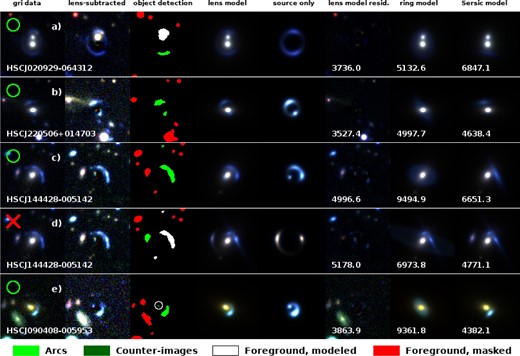
Steps of the lens-finding algorithm for a few example lenses and lens candidates. The first column shows the gri image of the system. The second column contains a lens-subtracted image, displayed with a different contrast to enhance features from lensed objects. The third column shows a segmentation map plot of the objects identified by SExtractor. Different colors represent candidate arcs, candidate counter-images to the main arc (only present in the fifth row, circled for better visibility), objects that are modeled as foreground, and foreground objects that are masked out, as specified in the legend. The fourth column shows the best-fitting lens model of the system, including models for foreground objects. The fifth column shows the best model of the lensed background galaxy alone, with the contrast set equal to the second column. The sixth column shows the residuals between the data and the best-fitting lens model. The seventh and eighth columns show the best-fitting ring and Sérsic models, respectively. The numbers at the bottom of the images in column six, seven and eight are the χ2 of the best-fitting model for the lens, ring, and Sérsic model, respectively. Circles in the top left-hand corner of each row indicate candidates that passed the selection. The cross in the fourth row indicates that the second interpretation of the image configuration for the lens candidate HSC J144428−005142 does not provide a good description of the system, since a model with a single Sérsic component at the position of the candidate arc gives a better fit. Even though the images are color-composite, only the g-band is used for the modeling of the arc-like features. The systems shown in rows (a), (b), and (e) are known lenses from the SL2S survey (More et al. 2012; Sonnenfeld et al. 2013a). The system in rows (c) and (d) is a new candidate found in HSC data. (Color online)
3.2 Lensed arc identification
We use SExtractor (Bertin & Arnouts 1996) to look for objects in the lens-subtracted g-band image. By using the g band we expect to detect lensed sources up to redshift z ∼ 4 (Ono et al. 2018). For each object we consider its position relative to the lens light centroid, its axis ratio and orientation, and the size of its footprint.
We then apply the following series of conditions to determine whether the object can be a lensed arc or not.
A distance from the lens centroid between 3 and 30 pixels (0|${^{\prime\prime}_{.}}$|50 < R < 5|${^{\prime\prime}_{.}}$|04).
A minimum ratio between the major and minor axis of 1.4.
A maximum difference of 30° between the position angle of the major axis of the object and the tangential to the circle centered on the lens and passing through the object centroid.
A minimum angular aperture, defined as the angle subtended by the object from the lens centroid, of 25°.
A footprint size between 20 and 500 pixels.
The minimum distance requirement in condition 1, as well as the minimum size requirement in condition 5, makes sure that the candidate arc is not just a residual from a non-perfect subtraction of the lens light. The maximum distance constraint is applied because we do not expect galaxy-scale lenses to have Einstein radii larger than 5″. Although there are lenses with larger Einstein radii, we typically refer to these as group-scale or cluster-scale lenses. Conditions 2 and 3 are applied to select only tangentially elongated objects. We add condition 4 to select objects that are elongated not just in terms of axis ratio, but that also describe a sizeable arc around the lens in angular terms. This conditions eliminates small objects far away from the lens that happen to pass the orientation and axis ratio requirement given by conditions 2 and 3 but are clearly not strongly lensed. Finally, we add the maximum size requirement in condition 5 to reject catastrophic failures in the object detection process. Objects that pass all five conditions are kept as potential arcs.
3.3 Foreground model
If the object detection process described above returned at least one arc candidate, we proceed with a more accurate fit of the lens light and by modeling potential foreground objects. We turn back to the i-band data and fit a Sérsic profile (Sérsic 1968) to the surface brightness distribution of the main galaxy, this time masking out any objects detected in the g-band image by SExtractor. We then go through non-arc-like objects detected in the i band around the lens, one by one in order of decreasing i-band flux, and fit each one with a Sérsic profile. Each time a new object is fitted, the structural parameters of the lens and previously fitted objects (i.e., centroid, effective radius, etc.) are kept fixed, as well as the relative i-band amplitude between the lens and any other object fitted up to that point. Only the overall amplitude of all previously fitted objects is varied. This prescription is adopted to reduce computation time. Only objects within 1.3 times the distance of the farthest arc-candidate of the lens are modeled. Objects farther away are simply masked out. Foreground objects other than the main galaxy are treated as massless: their contribution to the lens model, to be described in subsection 3.5, is ignored.
Although most known lenses do not have foreground objects other than the lens galaxy itself in the proximity of lensed images, accounting for the presence of foregrounds is important for the rejection of false-positive candidates. An example of foreground object modeling is shown in the first row of figure 1. After the lens light subtraction step, a galaxy is detected north of the lens and is then modeled with a Sérsic profile. The model of the lens and foreground object, together with a model for the lensed source to be described in subsection 3.5, is shown in the fourth column.
Up to this point, no color information has been used. Among the objects treated as foreground, there might be counter-images of the main arc. In the next subsection we will illustrate how we can classify images based on their color.
3.4 Multiple image set candidates
At this stage of the lens-finding process, we have candidate arcs and a model for the light distribution of the lens galaxy and surrounding objects. These objects can be either foreground objects or multiple images of the arcs. We use color and position information to distinguish between the two possibilities.
First of all, we apply a color selection to the arc candidates themselves. Since we expect lensed galaxies to be relatively blue we require a g − i color smaller than 2.0. Although a g − i color of 2.0 is not a particularly strong limit, it is sufficient to eliminate a frequent source of contaminants: satellite galaxies with their major axes oriented along the tangential direction. In principle, this color selection criterion could have been applied before the foreground object modeling step, in the interest of computation time. However, having an accurate model for the system is important to measure accurate colors and avoid rejecting good lenses for which the light from the arc happens to be contaminated by a foreground object. Fluxes in the i and g bands are measured by summing over pixels in the g-band footprint as determined by SExtractor. Although in principle we should match the PSF of the two bands for an accurate color measurement, the effect of differing PSFs is small with respect to the required precision. More important is the effect of modeling systematics from the subtraction of the light from the lens or foreground objects. To take this into account we add in quadrature to the statistical uncertainty on the flux of individual pixels a systematic uncertainty equal to 20% of the contribution from the best-fitting model of all light components.
We go through the blue (according to our color cut) arcs and create sets of arcs and non-arc objects with consistent g − i color, which we interpret as candidate sets of multiple images of the same source. We require colors of different objects to be within 2σ of each other in order to consider them consistent. The minimal multiple-image set consists of only one arc. If other candidate arcs are present, and if they have consistent g − i color, they are added to the set. An example of such a case is shown in the second row of figure 1: two objects satisfying the definition of arc given in subsection 3.2 are found by running SExtractor on the lens-subtracted image, shown in bright green in the segmentation map panel (third column). Since they have consistent colors, they are interpreted as multiple images of the same source.
If, on the contrary, there are arc-like objects with a different color than the arc defining the set, and if they are within 1.3 times the distance of the farthest arc from the lens, they are classified as foreground objects and are fitted with a Sérsic profile with the same procedure described in subsection 3.3. If these arc-like objects are at a farther distance from the lens, they are simply masked out. An example of this process is shown in the third and fourth rows of figure 1. For this lens candidate, our algorithm led to the detection of two potential arcs: an extended blue arc to the northwest of the main galaxy and a redder object to the east. Both objects could be lensed sources, but since they have different colors they cannot be multiple images of the same object. Then, two different interpretations are possible. If the bluer, bigger arc is the lensed source, then the red object must be a foreground object. Since it is too far away from the lens galaxy to affect any further analysis, it is simply masked out. This scenario is shown in the third row: the candidate arc is shown in bright green and objects masked out are shown in red. In the fourth row, the second interpretation is illustrated: the redder object is considered to be the lensed source, and the bluer elongated feature is modeled as a foreground object (marked in white in the segmentation map plot in addition to the main lens galaxy foreground).
Finally, we repeat the same procedure for non-arc-like objects: those with color consistent with the candidate arc(s) are assigned to a multiple image set. Objects with a different color are either modeled as foregrounds or masked out, depending on their distance from the lens galaxy. In the same system discussed above, a faint object is detected south of the lens. This is masked out in the first interpretation of the image configuration (third row of figure 1), but is modeled as a foreground in the second interpretation (fourth row), because its distance from the lens is within 1.3 times that of the main arc.
In the fifth row we show an instance of a system in which a non-arc-like object with color consistent to a candidate arc is found. The object is represented in dark green in the segmentation map plot. This object was modeled as a foreground in the previous step. However, since it is now treated as a counter-image of the arc, it is removed from the model of the foregrounds.
3.5 Lens model
We proceed to fit a lens model to each set of arcs and counter-images. The lens mass model consists of a singular isothermal ellipsoid (SIE), while the source surface brightness distribution is modeled with a circularly symmetric exponential profile. The centroid of the lens mass distribution is kept fixed to the value of the lens light centroid. The free parameters of the model then are: lens angular Einstein radius θE, axis ratio q, position angle PA, source position (sx, sy), and source effective radius se, as well as the amplitude of the source, lens and foreground surface brightness components. Foreground objects are treated as massless: only their surface brightness profile is modeled.
This is clearly a simplified model compared to what is usually needed to describe strong lens systems accurately, especially with respect to the source surface brightness distribution, a choice that is motivated by the computational time required to fit the data. However, as we will show later, it is not the absolute quality of a lens model that determines the outcome of the analysis by YattaLens but rather its relative quality compared to alternative non-lens models.
We use a modified version of the lens modeling code developed by Auger et al. (2011) to find a maximum-likelihood fit to the data. We explore the parameter space defined by the six non-linear parameters θE, q, PA, sx, sy, and se with an MCMC, where at each step of the chain we optimize for the amplitudes of the surface brightness components. As for the preliminary lens light subtraction step we use emcee to sample the posterior probability distribution of the model parameters, assuming flat priors on all of them.
This step of the algorithm is particularly slow. In order to minimize the cost in terms of time, we only run a relatively short chain, without ensuring that the MCMC has converged and that the true maximum likelihood model has been found. In order to maximize the chances of obtaining a good fit it is then important to find a reasonable starting solution. We use the following prescription to define our starting model. We set the initial mass orientation and axis ratio equal to that of the light distribution. Then, in case only one arc is present, we assume that the Einstein radius is equal to 0.7 times the distance of the arc from the lens. In case there are two or more arcs, the Einstein radius is set to the mean distance of the arcs from the lens. Once the lens mass parameters are set, the starting position of the source is found by mapping each arc centroid to the source plane and taking the mean of their position. We use the g-band image to perform the fit. Although the HSC i-band data has better image quality, we use the g band to minimize the contamination of the lensed images from the light of the lens galaxy and of foreground objects, which are typically redder than most lensed galaxies.
We then need to assess whether the best-fitting lens model is a good description of the data. In principle, we could use the χ2 to quantify the goodness-of-fit. In practice, with our simple model it is almost impossible to fit the image of a lens down to noise level, let alone do it automatically without human intervention. Therefore, instead of considering absolute values of the χ2, which have little meaning in this context, we compare the lens model χ2 with that obtained by fitting alternative models, described below. In principle, Bayesian evidence can be used to obtain a more accurate comparison between the different models. In practice, a simple χ2 analysis is sufficient for our purpose and is computationally faster than measuring the evidence.
3.6 Non-lens models
The lens candidates that have made it thus far are systems with a relatively blue, tangentially elongated object close to a massive galaxy. While some of these objects are indeed lenses, most of them are not. The two main sources of contaminants are (1) spiral arms (we will use the term spiral arm in a broad sense to indicate a mostly tangentially elongated star forming region) and (2) foreground galaxies with high ellipticity. The non-lens models that we compare against the lens model are designed to describe these two classes of systems.
Different realizations of a ring profile are shown in the seventh column of figure 1. While our lens model cannot produce radially elongated images, due to the upper limit on source size and the choice of a singular isothermal profile, the ring model has the ability of describing relatively large regions with approximately constant surface brightness. For example, for very large values of the inner scale radius ri, the ring profile reduces to a disk with approximately constant surface brightness within r0. Although hardly any galaxy can be described well by this surface brightness profile, the ring model provides a better fit compared to a lens model for most spiral galaxies that happen to be detected by the arc-finding step described in subsection 3.2, because it can provide a very rough description of their disk. An example of a galaxy with a candidate arc for which a ring model gives a better fit compared to a lens model is shown in figure 2.
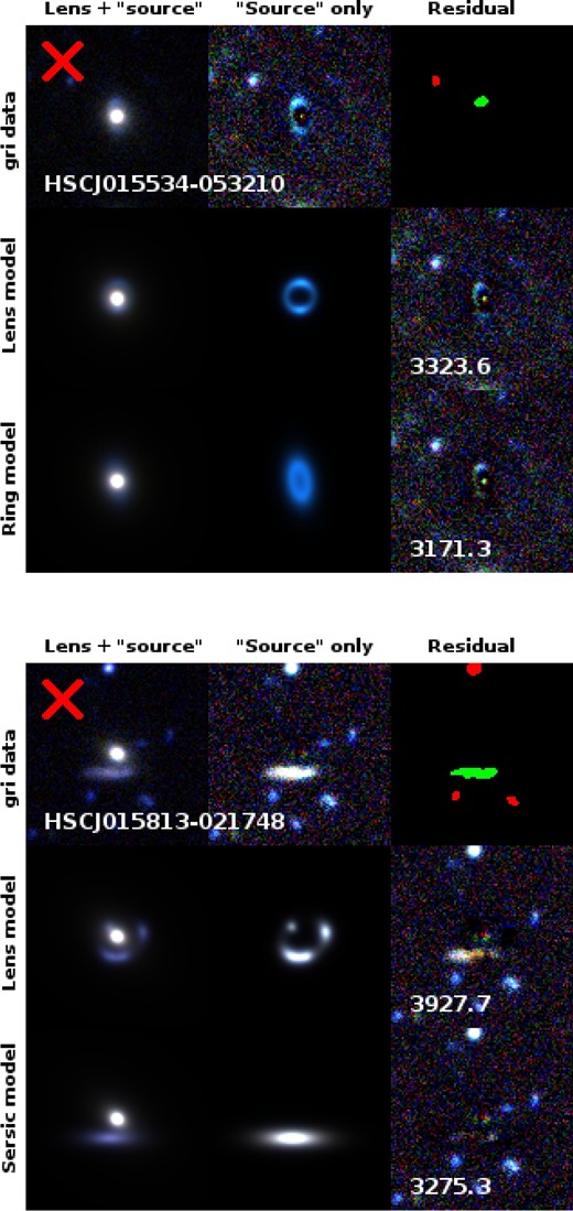
Lens candidates rejected by our algorithm because a ring (top panel) or a Sérsic (bottom panel) model provides a better fit compared to a lens model. The top row shows a gri image of the system, a lens-subtracted imaged, and a segmentation map showing the footprint of the identified candidate arc and that of masked-out object. The second row shows the best-fitting lens model of the system, the corresponding source-only image, and the residual. The third row in the top (bottom) panel shows the best-fitting ring (Sérsic) model, a ring-only (Sérsic-only) image, and the residual. (Color online)
When fitted to an actual lens, the ring model can hardly provide a reasonable fit. This is because the ring model is elliptically symmetric by construction, while the image configuration of strong lenses is not. The only case in which a ring profile could mimic a lens would be that of a perfectly circular Einstein ring. However, a perfect Einstein ring requires both a perfectly circular mass distribution and a perfect alignment between lens and source, an extremely rare circumstance.
The second non-lens model that we fit is a Sérsic profile with disky/boxy isophotes. Many arc candidates picked by the algorithm are just foreground objects with relatively high ellipticity that happen to be tangentially aligned with respect to the lens. A Sérsic profile provides a better fit with respect to a lens model for most of these systems. One such example is shown in figure 2, while another instance appears in the fourth row of figure 1, where the object interpreted as an arc is better fitted by a Sérsic component.
3.7 A summary of the algorithm
We have described in detail all the steps taken by YattaLens to look for strong lenses. Let us summarize the steps of the algorithm.
Given a massive galaxy, YattaLens fits a de Vaucouleurs profile to its i-band surface brightness profile, then subtracts the best-fitting model from the g-band image. This step takes a few seconds on a standard machine.
SExtractor is run on the lens-subtracted g-band image to look for tangentially elongated objects within ∼5″. This step takes a fraction of a second.
If a candidate arc is found, YattaLens proceeds to model any object within a region where potential counter-images of the arc could be, then measures colors of arcs and other objects. This step can take from a few seconds to a few minutes, depending on how many foreground objects are present.
If the candidate arc is bluer than g − i = 2, YattaLens makes sets of arcs and images of consistent color. For each multiple image set, any other object with inconsistent color is either modeled as a foreground object or masked out, depending on the ratio between its distance from the lens and the distance of the farthest candidate arc from the lens.
For each multiple image set, the g-band image is fitted with a lens model, a ring model, and a Sérsic model. Each model includes a model of the lens galaxy and possible foreground objects, described as the sum of Sérsic profiles with fixed relative amplitude. It takes about a minute to run this modeling step.
If the lens model provides a better fit, in terms of χ2, with respect to both the ring and the Sérsic model, the candidate is selected. Otherwise it is rejected.
In the next subsection we will show how YattaLens performs on a sample of known lenses.
3.8 Tests on known lenses
The YattaLens algorithm has been tested on a sample of known lenses that lie in the S16A data release of HSC. These are 16 galaxy-scale lenses from the SL2S survey (SL2S J021247−055552, SL2S J021411−040502, SL2S J021737−051329, SL2S J022357−065142, SL2S J022511−045433, SL2S J022610−042011, SL2S J022648−040610, SL2S J022708−065445, SL2S J023251−040823, SL2S J023307−043838, SL2S J090407−005952, SL2S J142003+523137, SL2S J220329+020518, SL2S J220506+014703, SL2S J221326−000946, SL2S J222148+011542: Gavazzi et al. 2012; Sonnenfeld et al. 2013a, 2015), plus the double source plane lens HSC J142449−005322 also known as the “Eye of Horus” (Tanaka et al. 2016).
YattaLens was able to identify 15 lenses correctly out of 17. The two systems missed by YattaLens are SL2S J022357−065142 and SL2S J022708−065445. Both were missed during the arc-detection step, the arcs being too faint to be picked out by SExtractor, which we run with a detection threshold of 2σ above the background. The images of these two lenses, which were originally discovered using Ringfinder are shown in figure 3.
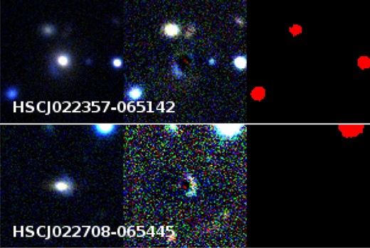
Known strong lenses from the SL2S survey missed by YattaLens. The left-hand panels show a color-composite gri HSC image of the systems, the middle panels show lens-subtracted images with enhanced contrast, and the right-hand panels show the segmentation map obtained by running SExtractor on the g-band lens-subtracted images. The arcs are not detected. (Color online)
In figure 4 we show YattaLens’ analysis on the double source plane lens the Eye of Horus. Double source plane lenses are very interesting objects because they offer more constraints with respect to typical lenses, and can be used for detailed studies of the mass distribution of the foreground galaxy (e.g., Sonnenfeld et al. 2012), or to infer cosmological parameters (Gavazzi et al. 2008; Collett & Auger 2014; Schneider 2014). Since they are also very rare, it is extremely important that lens-finding algorithms do recognize them as lenses. This can be challenging for automatic algorithms because the presence of arcs from more than one source complicate their morphology. Therefore, we made sure when designing YattaLens that it could properly classify the Eye of Horus, the only spectroscopically confirmed double source plane lens in the HSC survey, as a lens.
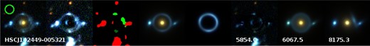
YattaLens analysis of the double source plane lens “The Eye of Horus” (Tanaka et al. 2016). Panels are the same as figure 1. As can be seen from the segmentation map (third panel), YattaLens correctly identifies part of the outer ring as an arc. The bright knot on the southern part of the outer ring is also correctly identified as a counter-image. The eastern bright knot, however, is classified as a contaminant, due to an inaccurate estimate of the color. Nevertheless, the lens model provides a better fit compared to both the ring model (column seven) and the Sérsic model (column eight) and the system is correctly classified as a lens. (Color online)
Since most of the SL2S lenses in HSC are recovered, we can deduce that the completeness of YattaLens is comparable to that of Ringfinder. We cannot draw more quantitative statements on completeness at this stage because (1) the SL2S lenses have been used to optimize the parameters of the algorithm and (2) the SL2S sample is not a complete sample in the first place, meaning that there could be lenses missed by Ringfinder that YattaLens would be able to identify. In order to determine the completeness of a lens search with YattaLensrobustly, we need to run the algorithm on a realistic simulation of a large set of lenses. This is left for future work.
4 CHITAH
Chitah (Chan et al. 2015) is a lens hunter in imaging surveys, which was originally developed for lensed quasars, based on the configuration of lensed images. Not only lensed quasars, but also lensed galaxies can be captured when Chitah identifies lensed images within a lensed arc. Briefly, the procedure of Chitah is as follows.
Choose two image cutouts, one from bluer bands (g/r) and one from redder bands (z/y) which have sharper PSFs.
Match PSFs in the two selected bands.
Disentangle the lens light and lensed arc image according to color information, producing a “lens” image and a “lensed arc” image.
Identify the lens center and lensed image positions, masking out the region within 0|${^{\prime\prime}_{.}}$|5 in radius from the lens center in the lensed arc image to prevent misidentifying lensed image positions near the lens center due to imperfect lens light separation.
Model the lensed image configuration with an SIE lens mass distribution.
The criteria of classification of lens candidates are |$\chi ^2_{\rm src}+\chi _{\mathrm{c}}^2 < 2 \theta _{\rm E}$|, where θE is measured in arcsec, and χres2 < 100. The former criterion allows Chitah to detect lens candidates covering a wide range of θE, since typically |$\chi ^2_{\rm src}$| scales with θE and our tests with mock systems in Chan et al. (2015) show that |$\chi ^2_{\rm src} \lesssim 4$| yields a low false-positive rate of <3%. The latter criterion allows us to further eliminate false positives. The lens candidates are selected within 0|${^{\prime\prime}_{.}}$|3 < θE < 4″.
5 Spectroscopic search
Another powerful and efficient lens search method is the spectroscopic selection technique developed by Bolton et al. (2004). This spectroscopic selection technique has led to discoveries of almost 200 strong lenses in several dedicated lens surveys including the Sloan Lens ACS Survey (SLACS: Bolton et al. 2008), the Sloan WFC Edge-on Late-type Lens Survey (SWELLS: Treu et al. 2011), the SLACS for the Masses Survey (S4TM: Shu et al. 2015), the BOSS Emission-Line Lens Survey (BELLS: Brownstein et al. 2012), and the BELLS for GAlaxy-Lyα EmitteR sYstems Survey (BELLS GALLERY: Shu et al. 2016a, 2016b). Here we describe briefly the spectroscopic selection algorithm implemented in this work. More technical details can be found in Bolton et al. (2004) and Shu et al. (2016a).
For each observed spectrum, the best-fitting galaxy template from the BOSS data reduction pipeline (Bolton et al. 2012a) is subtracted to obtain its residual spectrum. An error-weighted matched-filter search for emission-line features is performed on the residual spectrum. Note that flux errors are rescaled in this step because the BOSS pipeline-reported errors are usually underestimated at wavelengths with strong airglow lines. The rescaling process is detailed in Shu et al. (2016a). Emission-line detections with a signal-to-noise ratio (SNR) greater than 4 are retained and referred to as “hits”. In previous lens surveys, galaxies with either multiple hits (SLACS, SWELLS, S4TM, BELLS) or a single hit (BELLS GALLERY) are targeted because they fall into different lens categories. The background sources are star-forming galaxies for multiple-hit systems, and Lyα emitters for single-hit systems. However, as the purpose of this work is to find as many strong lenses as possible, we keep all the targets with at least one hit as lens candidates. Further visual inspections on their HSC images will confirm the lens nature.
6 Results
We ran YattaLens, Chitah, and the spectroscopic search method on a sample of ∼43000 massive galaxies from the BOSS survey. A first set of ∼8000 objects was used to further optimize YattaLens, in particular to improve its purity, i.e., to reduce the number of false positives. Once the algorithm was stable we applied it to the full sample. YattaLens found 1480 lens candidates, of which 250 were from the LOWZ subsample and 1230 were from CMASS. Chitah found 819, while the spectroscopic method found 233. Of these candidates, 118 were common to at least two methods and three were found by all three.
10 of these candidates are known lenses. They are six galaxy-scale SL2S lenses (SL2S J021411−040502, SL2S J021737−051329, SL2S J022346−053418, SL2S J022511−045433, SL2S J023307−043838, and SL2S J220506+014703), the Eye of Horus lens HSC J142449−005321, already discussed in subsection 3.8, and three group-scale lenses from the Strong Lensing Legacy Survey - ARCS (SARCS) sample (SL2S J020929−064312, SL2S J021408−053530, SL2S J221418+011036: More et al. 2012). All of these were identified by YattaLens and two of them were found by Chitah as well.
We visually inspected the remaining lens candidates and graded them according to their likelihood of being strong lenses, Plens, using the following scheme:
Grade A: definite lenses (Plens > 0.997),
Grade B: probable lenses (0.5 < Plens < 0.997),
Grade C: possible lenses (0.003 < Plens < 0.5),
Grade 0: non-lenses (Plens < 0.003).
A first classification was done using the image configuration as the only criterion to establish the likelihood of a candidate being a lens. Typical aspects that are taken in consideration are: the curvature and orientation of the candidate arc, the presence of counter-images at the opposite position to the main arc with respect to the lens, and the presence of spiral arms or a disk component (suggesting that the system is not a lens). Nine people independently graded each candidate, assigning an integer score between 0 and 3 (0 corresponding to Grade 0, 1 to Grade C, 2 to Grade B, and 3 to Grade A). A first list of grade A, B, and C systems was compiled, taking the average score among the graders, rounded to the nearest integer (i.e., systems with an average score strictly larger than 2.5 are temporarily labeled as Grade A).
We then visually inspected the spectra of the grade A, B, and C candidates with emission-line detections, as well as the grade A and B candidates from YattaLens and Chitah, to determine whether these detections are robust and, if so, to measure the redshift of the candidate lensed source. Since we use a relatively low SNR threshold in the emission line detection algorithm, most of the candidate lines could not be confirmed by eye. The few systems with unambiguous line detections showed only one line. Roughly half of these lines showed a double-peak profile typical of the [O ii] doublet at 3727 Å. We measured their redshift based on this interpretation. The remaining lines were all detected at a wavelength bluer than 5100 Å. In those cases we assumed the line to be Ly-α.
We found eight objects with visually confirmed emission lines from an object at a higher redshift than the source, all of which were already part of the emission line selected sample. We then discussed the grade A, B, and C list in light of this additional information. Candidates HSC J085855−010208 and HSC J141815+015832 were upgraded from B to A, while HSC J144307−004056 was upgraded from C to B. In making the final grade A list we added a unanimity requirement: all people taking part in the grading must agree on the lens nature of grade A systems.
Table 1 lists the number of candidates of each grade found by each method. We found 15 new grade A (definite) lenses, 36 grade B (probable) lenses, and 282 grade C (possible) lenses. Grade A lenses are shown figure 5 while grade B candidates are shown in figure 6. Their basic properties are listed in table 2. The full list of candidates including grade C systems can be found online.1
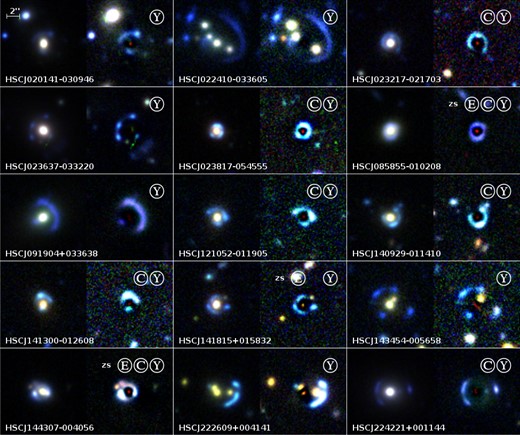
Grade A lenses. For each system, the left-hand panel is a color-composite image in g, r, and i bands, while the right-hand panel is a lens-subtracted version of the image. A higher contrast is used in the right-hand panel to enhance the images of the lensed source. Circled letters on the top of each image indicate whether the lens was found by YattaLens (Y), Chitah (C), or the emission-line search (E). The letters “zs” indicate systems for which a spectroscopic redshift of the source galaxy has been measured. (Color online)


Grade B candidates. For each system, the left-hand panel is a color-composite image in g, r, and i bands, while the right-hand panel is a lens-subtracted version of the image. A higher contrast is used in the right-hand panel to enhance the images of the lensed source. Circled letters on the top of each image indicate whether the lens candidate was found by YattaLens (Y), Chitah (C) or the emission-line search (E). The letters “zs” indicate systems for which a spectroscopic redshift of the source galaxy has been measured. (Color online)
Lens candidate statistics.*
| YattaLens | Chitah | Emission line | Total | |
|---|---|---|---|---|
| Candidates | 1480 | 819 | 233 | 2411 |
| Grade A | 15 | 8 | 3 | 15 |
| Grade B | 31 | 10 | 3 | 36 |
| Grade C | 217 | 39 | 49 | 282 |
| Known | 10 | 2 | 0 | 10 |
| YattaLens | Chitah | Emission line | Total | |
|---|---|---|---|---|
| Candidates | 1480 | 819 | 233 | 2411 |
| Grade A | 15 | 8 | 3 | 15 |
| Grade B | 31 | 10 | 3 | 36 |
| Grade C | 217 | 39 | 49 | 282 |
| Known | 10 | 2 | 0 | 10 |
*Number of lens candidates found by each search method. The first row lists the number of candidates that have been visually inspected. The second to fourth rows list the numbers of grade A, B, and C lenses, respectively. The fifth row lists the number of previously known lenses that have been recovered.
Grade A lenses and grade B candidates.*
| Name | RA (|$^{\rm h}\phantom{0}^{\rm m}\phantom{0}^{\rm s}$|) | Dec (|$^{\circ}\phantom{0}^{\prime}\phantom{0}^{\prime\prime}$|) | zd | zs | Subsample | PDR1 | Grade | YL | EM | CH |
|---|---|---|---|---|---|---|---|---|---|---|
| HSC J015731−033057 | 01:57:31.49 | −03:30:57.66 | 0.621 | — | CMASS | N | B | Y | N | N |
| HSC J015756−021809 | 01:57:56.61 | −02:18:09.96 | 0.372 | — | LOWZ | N | B | N | N | Y |
| HSC J020141−030946 | 02:01:41.98 | −03:09:46.05 | 0.362 | — | LOWZ | N | A | Y | N | N |
| HSC J020241−064611 | 02:02:41.39 | −06:46:11.24 | 0.502 | 2.75 | CMASS | N | B | Y | Y | N |
| HSC J020846−032727 | 02:08:46.85 | −03:27:27.68 | 0.618 | — | CMASS | Y | B | Y | N | N |
| HSC J022140−021020 | 02:21:40.13 | −02:10:20.10 | 0.708 | — | CMASS | N | B | Y | N | N |
| HSC J022410−033605 | 02:24:10.37 | −03:36:05.31 | 0.613 | — | CMASS | Y | A | Y | N | N |
| HSC J023217−021703 | 02:32:17.37 | −02:17:03.72 | 0.508 | — | CMASS | N | A | Y | N | Y |
| HSC J023538−063406 | 02:35:38.22 | −06:34:06.07 | 0.181 | — | LOWZ | N | B | Y | N | N |
| HSC J023637−033220 | 02:36:37.30 | −03:32:20.04 | 0.270 | — | LOWZ | N | A | Y | N | N |
| HSC J023655−023656 | 02:36:55.27 | −02:36:56.01 | 0.562 | — | CMASS | N | B | Y | N | N |
| HSC J023817−054555 | 02:38:17.77 | −05:45:55.52 | 0.599 | — | CMASS | N | A | Y | N | Y |
| HSC J083726+015639 | 08:37:26.18 | 01:56:39.46 | 0.395 | — | LOWZ | N | B | Y | N | N |
| HSC J083943+004740 | 08:39:43.03 | 00:47:40.79 | 0.621 | — | CMASS | N | B | N | N | Y |
| HSC J085855−010208 | 08:58:55.99 | −01:02:08.42 | 0.468 | 1.42 | CMASS | N | A | Y | Y | Y |
| HSC J090507−001030 | 09:05:7.35 | −00:10:30.03 | 0.494 | — | CMASS | Y | B | Y | N | Y |
| HSC J090613+032939 | 09:06:13.14 | 03:29:39.98 | 0.617 | — | CMASS | N | B | N | N | Y |
| HSC J090709+005648 | 09:07:9.70 | 00:56:48.42 | 0.478 | — | CMASS | Y | B | Y | N | Y |
| HSC J091904+033638 | 09:19:4.60 | 03:36:38.65 | 0.444 | — | LOWZ | N | A | Y | N | N |
| HSC J115214+003126 | 11:52:14.19 | 00:31:26.49 | 0.466 | — | CMASS | N | B | N | Y | N |
| HSC J115653−003948 | 11:56:53.03 | −00:39:48.51 | 0.508 | — | CMASS | Y | B | Y | N | N |
| HSC J120623+001507 | 12:06:23.85 | 00:15:07.15 | 0.563 | 3.12 | CMASS | N | B | N | Y | N |
| HSC J121052−011905 | 12:10:52.49 | −01:19:05.17 | 0.700 | — | CMASS | N | A | Y | N | Y |
| HSC J140929−011410 | 14:09:29.71 | −01:14:10.72 | 0.584 | — | CMASS | N | A | Y | N | Y |
| HSC J141300−012608 | 14:13:0.07 | −01:26:08.16 | 0.749 | — | CMASS | N | A | Y | N | Y |
| HSC J141635+010128 | 14:16:35.43 | 01:01:28.91 | 0.700 | — | CMASS | N | B | Y | N | N |
| HSC J141728+015935 | 14:17:28.10 | 01:59:35.28 | 0.401 | — | LOWZ | N | B | Y | N | N |
| HSC J141815+015832 | 14:18:15.73 | 01:58:32.30 | 0.556 | 2.14 | CMASS | N | A | Y | Y | N |
| HSC J141831−000052 | 14:18:31.41 | −00:00:52.65 | 0.263 | — | LOWZ | Y | B | Y | N | N |
| HSC J142053+005620 | 14:20:53.62 | 00:56:20.63 | 0.616 | — | CMASS | Y | B | Y | N | N |
| HSC J142720+001916 | 14:27:20.55 | 00:19:16.11 | 0.551 | — | CMASS | Y | B | Y | N | N |
| HSC J142748+000958 | 14:27:48.36 | 00:09:58.76 | 0.589 | — | CMASS | Y | B | Y | N | N |
| HSC J143454−005658 | 14:34:54.40 | −00:56:58.56 | 0.728 | — | CMASS | Y | A | Y | N | N |
| HSC J144307−004056 | 14:43:7.16 | −00:40:56.10 | 0.500 | 1.07 | CMASS | Y | A | Y | Y | Y |
| HSC J144428−005142 | 14:44:28.74 | −00:51:42.45 | 0.575 | — | CMASS | N | B | Y | N | N |
| HSC J145236−002142 | 14:52:36.66 | −00:21:42.04 | 0.733 | — | CMASS | N | B | Y | N | N |
| HSC J145732−015917 | 14:57:32.58 | −01:59:17.36 | 0.526 | — | CMASS | N | B | Y | N | Y |
| HSC J145836−002400 | 14:58:36.29 | −00:24:00.77 | 0.595 | — | CMASS | N | B | Y | N | N |
| HSC J145902−012351 | 14:59:2.72 | −01:23:51.17 | 0.482 | — | CMASS | N | B | Y | N | N |
| HSC J155319+431824 | 15:53:19.39 | 43:18:24.31 | 0.629 | — | CMASS | N | B | Y | N | N |
| HSC J155517+415138 | 15:55:17.74 | 41:51:38.71 | 0.555 | — | CMASS | N | B | Y | N | Y |
| HSC J155826+432830 | 15:58:26.66 | 43:28:30.83 | 0.444 | — | LOWZ | N | B | Y | N | Y |
| HSC J155957+441543 | 15:59:57.55 | 44:15:43.81 | 0.598 | — | CMASS | N | B | Y | N | N |
| HSC J221726+000350 | 22:17:26.44 | 00:03:50.33 | 0.398 | — | LOWZ | Y | B | Y | N | Y |
| HSC J222609+004141 | 22:26:9.30 | 00:41:41.99 | 0.647 | — | CMASS | Y | A | Y | N | N |
| HSC J222801+012805 | 22:28:1.98 | 01:28:05.74 | 0.647 | — | CMASS | Y | B | Y | N | Y |
| HSC J223518−004747 | 22:35:18.31 | −00:47:47.30 | 0.640 | — | CMASS | N | B | Y | N | N |
| HSC J223733+005015 | 22:37:33.54 | 00:50:15.78 | 0.604 | — | CMASS | Y | B | Y | N | N |
| HSC J224201+022810 | 22:42:1.18 | 02:28:10.61 | 0.443 | — | LOWZ | N | B | Y | N | N |
| HSC J224221+001144 | 22:42:21.58 | 00:11:44.71 | 0.385 | — | LOWZ | Y | A | Y | N | Y |
| HSC J224858+014711 | 22:48:58.98 | 01:47:11.27 | 0.360 | — | LOWZ | N | B | Y | N | N |
*Columns 2 and 3: Lens coordinates. Columns 4 and 5 list lens and source redshift (when measured), respectively. Column 6 lists which subsample of BOSS LRGs the lens galaxy belongs to. Column 7 indicates whether the system lies in the region covered by the public data release 1 or not. Column 8 indicates the grade of the candidate. Columns 9, 10, and 11 indicate if the candidate was identified by YattaLens, by the emission-line search method, or by Chitah, respectively.
The 15 grade A lenses exhibit regular surface brightness profiles in their lensed sources, bright arcs and counter-images with positions and shapes expected for a smooth lensing potential, and, in three cases, emission lines from the background source. The 36 grade B candidates, although very promising systems and most likely lenses, show features that leave room for ambiguity in their classification. These features are arcs that appear to extend excessively for a smooth mass distribution (for example HSC J015731−033057 and HSC J022140−021020), arcs that appear to have too little curvature (HSC J141635+010128, HSC J223733+005015), the absence of visible counter-images (HSC J020846−032727, HSC J144428−005142), or lensed images that are simply too faint to allow for an unambiguous classification. Higher-resolution imaging data, or spectroscopic observations of the lensed arcs with a broad wavelength coverage, is needed to confirm the lens nature of these systems.
7 Discussion
We applied three different lens-finding algorithms to the same photometric and spectroscopic dataset, finding 51 definite/probable lenses. This sample is large enough for us to gain valuable information on the relative efficiency of the three algorithms. In particular we can focus on the relative completeness, defined as the number of highly probable lenses found by one algorithm divided by the number of lenses found by all three combined.
YattaLens has the highest relative completeness, with 46 systems identified out of 51. In comparison, Chitah found 18 systems, while the emission-line search produced six good candidates. This result is not surprising because YattaLens was specifically developed for this study. In contrast, Chitah has been optimized to look for lensed quasars. In this respect, it is remarkable that Chitah was able to find as many as 18 lenses, most of which are not lensed quasars. The emission-line search method instead relies entirely on the presence of emission lines from the lensed source in the 2|${^{\prime\prime}_{.}}$|0 diameter optical fiber of BOSS (Smee et al. 2013). The likelihood of a detection depends first of all on the redshift of the source (no significant emission lines fall in the optical part of the spectrum for objects in the redshift range 1.5 ≲ z ≲ 2.5), but also on the Einstein radius and image configuration of the lens: lensed images too far out from the fiber do not leave a trace on the BOSS spectrum. It is then not surprising that the emission-line search missed many lenses, a good fraction of which have relatively large Einstein radii. Nevertheless, it provided us with three highly probable lenses undetected by the other two methods.
Another important aspect to consider is purity, defined as the ratio between the number of true lenses and the total number of candidates returned by a lens-finding algorithm. Again, it is not possible with this data alone to establish the absolute purity achieved by our search methods because for a large number of candidates, particularly the grade C candidates, we cannot determine with absolute certainty whether they are lenses or not. However, as a proxy for purity we can consider the ratio between the number of candidates with grade B or above and the total number of candidates. YattaLens achieved the highest ratio, with 3.1% of the candidates being grade B lenses or better (3.7% if we consider the 10 known lenses recovered), compared to 2.6% for the emission-line search method and 2.2% for Chitah (2.4% counting the two known lenses). Another way to interpret this result is that YattaLens required the least amount of visual inspection to find the same number of lenses, compared to the other methods. In the next two subsections we will focus on some more aspects of our lens-finding algorithm.
7.1 Lenses missed by YattaLens
YattaLens identified all of the new grade A lenses we discovered, but missed five grade B candidates. Here we discuss briefly what went wrong with each of these systems.
HSC J015756−021809. This system was found by Chitah. Although YattaLens correctly detected a candidate arc around the lens galaxy, it was discarded because the ring model fit gave a better χ2 compared to the lens model fit.
HSC J083943+004740. This lens consists of a doubly imaged compact source, probably a quasar, and was discovered by Chitah. The two images were correctly detected by YattaLens but since they are not tangentially elongated they were not classified as candidate arcs.
HSC J090613+032939. This lens was also identified by Chitah. The main arc was detected by YattaLens but was then discarded after the modeling step, since the ring model produced a better fit to the data compared to the lens model. The arc is relatively faint in the g band, which is used for the modeling step. If the z and i bands are used for the modeling of the lens and arc light, respectively, YattaLens recovers this candidate.
HSC J115214+003126. The main candidate arc is too faint and was not detected by SExtractor. Incidentally, although this system was found by the emission-line search algorithm, the candidate arc is very faint and is located 5″ away from the lens. It is then unlikely that a signal from the source galaxy was detected in the BOSS spectrum. Indeed, visual inspection of the spectrum did not show any convincing emission lines. It is then possible that the presence of the arc is a fortuitous coincidence.
HSC J120623+001507. Similarly to HSC J083943+004740, this doubly imaged compact source was not recognized as a candidate arc by YattaLens due to the absence of any tangential elongation.
7.2 The performance of YattaLens
As described extensively in section 3, YattaLens consists of two main steps: candidate arc detection and lens modeling. Of the initial ∼43000 systems, YattaLens detected arcs in 5097 of them. Of these arcs, 346 were discarded because they were deemed too red, while the remaining 4751 were modeled. After the modeling, the sample size was reduced to 1480 systems, which were then visually inspected. Of these systems, 273 were classified as possible lenses: grade C or above.
The modeling step reduced the number of candidates by more than a factor of 3 with respect to a selection based only on the presence of arc-like features. This is a significant improvement in terms of human time needed to inspect candidates visually. Although only 20% of the systems returned by YattaLens turned out to be possible lenses, this fraction is almost a factor of 2 larger than what was achieved by Ringfinder with similar data from CFHT (Gavazzi et al. 2014).
Such an improvement in purity was accompanied by a modest loss in completeness. Among the 22 grade B or above lenses found by either Chitah or the emission-line method, two were discarded by YattaLens during the modeling step. Although the statistics are too small to draw a robust conclusion, analysis of this sample suggests that such a loss in completeness is probably small.
7.3 Distribution in z–M* space
In figure 7 we plot the distribution in redshift and stellar mass of the newly found lenses, compared with the distribution of the parent sample of galaxies and of existing samples of lenses. In particular we consider the BELLS sample, which is also a lens-selected sample based on BOSS LRGs, and the SL2S sample. Stellar masses for the SuGOHI-g and the BELLS lenses are taken from Maraston et al. (2013) and are based on spectro-photometric fitting and a Salpeter IMF. Stellar masses based on a Salpeter IMF for the SL2S lenses are taken from Sonnenfeld et al. (2013a).
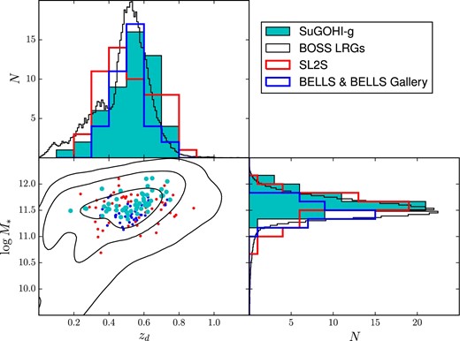
Distribution in lens redshift and stellar mass of SuGOHI-g lenses, SL2S lenses, BELLS lenses, and BOSS LRGs. The histograms of the BOSS LRGs’ distribution have been rescaled by an arbitrary constant. (Color online)
SuGOHI-g lenses, as well as lenses from BELLS and SL2S, are located at the high end of the mass distribution. This is expected from a lensing cross-section argument: more massive objects are more likely to be strong lenses and can give rise to sets of multiple images with larger separation, and are thus more easily detectable. The redshift distribution of SuGOHI-g lenses is similar to that of its parent sample, BOSS LRGs, suggesting that lensing selection and the efficiency of our lens finders do not strongly favor a particular region in redshift space.
8 Conclusions and future prospects
We looked for strong gravitational lenses in the first public data release of the HSC survey. We applied three different lens search methods to a sample of 43000 BOSS LRGs with HSC imaging. The first method is a new lens-finding algorithm, YattaLens, developed specifically for this study. YattaLens looks for blue, tangentially elongated features around massive galaxies, then fits a lens model to determine whether the identified features could be strongly lensed images of background galaxies. Unlike other modeling-based lens finders, YattaLens does not try to determine the likelihood of an object being a lens based on the absolute quality of a lens model fit, but only in relation to alternative models. These models are a single Sérsic component and a profile describing the disk component of a late-type galaxy.
The second method used in the lens search is Chitah, a modeling-based algorithm originally developed to look for lensed quasars but capable of finding lensed galaxies as well. The third method is based on the detection of emission lines from objects at a higher redshift than the main galaxy in BOSS spectroscopy data, a method that has been used successfully in various lens search campaigns.
The three methods selected a total of ∼2400 candidates which were then visually inspected. We found 15 new definite (grade A) lenses and 36 new highly probable (grade B) lenses. YattaLens achieved the highest completeness and purity among the three methods, with 46 grade A and B lenses out of 1480 candidates, but still missed five grade B lenses that were recovered by the other two methods.
These results are very promising in view of the advancement of the HSC-SSP campaign. The current lens search has been carried out on a 442 deg2 area. As the HSC survey progresses to its final coverage of 1400 deg2, we expect a corresponding increase in the number of lenses of more than a factor of 3. This number is likely to be a lower limit, because ∼60% of the data used in our search is shallower than the planned survey depth, potentially resulting in a decreased completeness. Another boost in the number of lenses can be obtained by selecting targets using photometric information alone, instead of relying on BOSS spectroscopy. For instance, the completeness of the BOSS CMASS sample at z = 0.6 and at the mean stellar mass of the SuGOHI-g sample is 60% (Leauthaud et al. 2016), suggesting that selecting lens candidates using photometric redshifts could lead to an increase in sample size by almost a factor of 2. This estimate is consistent with results from the SL2S survey: of the 21 grade B or above lenses in the W1 field of CFHTLS, uniformly covered by BOSS, only 11 have BOSS spectroscopy data. Given these considerations, since our lens finders were able to detect 61 grade B or above lenses (including the 10 known) among BOSS LRGs with HSC 2016A data, we expect the SuGOHI-g sample to grow to a size of at least ∼300 by the end of the HSC survey and by extending the search to photometrically selected massive galaxies. This number is significantly more than the largest samples of lenses known to-date.
Acknowledgements
The Hyper Suprime-Cam (HSC) collaboration includes the astronomical communities of Japan and Taiwan, and Princeton University. The HSC instrumentation and software were developed by the National Astronomical Observatory of Japan (NAOJ), the Kavli Institute for the Physics and Mathematics of the Universe (Kavli IPMU), the University of Tokyo, the High Energy Accelerator Research Organization (KEK), the Academia Sinica Institute for Astronomy and Astrophysics in Taiwan (ASIAA), and Princeton University. Funding was contributed by the FIRST program from the Japanese Cabinet Office, the Ministry of Education, Culture, Sports, Science, and Technology (MEXT), the Japan Society for the Promotion of Science (JSPS), the Japan Science and Technology Agency (JST), the Toray Science Foundation, NAOJ, Kavli IPMU, KEK, ASIAA, and Princeton University.
Funding for SDSS-III has been provided by the Alfred P. Sloan Foundation, the Participating Institutions, the National Science Foundation, and the U.S. Department of Energy Office of Science. The SDSS-III web site is 〈http://www.sdss3.org/〉.
SDSS-III is managed by the Astrophysical Research Consortium for the Participating Institutions of the SDSS-III Collaboration including the University of Arizona, the Brazilian Participation Group, Brookhaven National Laboratory, Carnegie Mellon University, the University of Florida, the French Participation Group, the German Participation Group, Harvard University, the Instituto de Astrofisica de Canarias, the Michigan State/Notre Dame/JINA Participation Group, Johns Hopkins University, the Lawrence Berkeley National Laboratory, the Max Planck Institute for Astrophysics, the Max Planck Institute for Extraterrestrial Physics, New Mexico State University, New York University, Ohio State University, Pennsylvania State University, the University of Portsmouth, Princeton University, the Spanish Participation Group, the University of Tokyo, the University of Utah, Vanderbilt University, the University of Virginia, the University of Washington, and Yale University.
This work was supported by the World Premier International Research Center Initiative (WPI Initiative), MEXT, Japan. JHHC and SHS gratefully acknowledge the support from the Max Planck Society through the Max Planck Research Group for SHS, and support from the Ministry of Science and Technology in Taiwan via grant MOST-103-2112-M-001-003-MY3. YS is partially supported by the National Natural Science Foundation of China (NSFC) grant 11603032. This work was supported in part by JSPS KAKENHI Grant Number 26800093 and 15H05892. KCW is supported by an EACOA Fellowship awarded by the East Asia Core Observatories Association, which consists of the Academia Sinica Institute of Astronomy and Astrophysics, the National Astronomical Observatory of Japan, the National Astronomical Observatories of the Chinese Academy of Sciences, and the Korea Astronomy and Space Science Institute.
Footnotes
References
