


Abstract
We utilize the Hyper Suprime-Cam (HSC) CAMIRA cluster catalog (Oguri et al. 2018 PASJ, 70, S20) and the photo-z galaxy catalog constructed in the HSC Wide field (S16A), covering ∼174 deg2, to study the star formation activity of galaxies in different environments over 0.2 < z < 1.1. We probe galaxies down to i ∼ 26, corresponding to a stellar mass limit of log10(M*/M⊙) ∼ 8.2 and ∼8.6 for star-forming and quiescent populations, respectively, at z ∼ 0.2. The existence of the red sequence for low stellar mass galaxies in clusters suggests that the environmental quenching persists to halt the star formation in the low-mass regime. In addition, star-forming galaxies in groups or clusters are systematically biased toward lower values of specific star formation rate by 0.1–0.3 dex with respect to those in the field, and the offsets show no strong redshift evolution over our redshift range, implying a universal slow quenching mechanism acting in the dense environments since z ∼ 1.1. Moreover, the environmental quenching dominates the mass quenching in low-mass galaxies, and the quenching dominance reverses in high-mass ones. The transition mass is greater in clusters than in groups, indicating that the environmental quenching is more effective for massive galaxies in clusters compared to groups.
1 Introduction
It is well established that clusters at z < 1 are dominated by galaxies with redder colors, older stellar populations, early type morphologies, and little star formation, as opposed to the field environments. Many scenarios related to cluster environments have been proposed to explain how the star formation is halted in clusters, including processes, such as ram-pressure stripping (Gunn & Gott 1972; Dressler & Gunn 1983), and galaxy–galaxy interaction (Mihos & Hernquist 1994), that quench star formation over a short timescale, and ‘strangulation’, referring to the removal of warm and hot gas (Larson et al. 1980; Balogh et al. 2000), which slowly reduces the cold gas supply. Studying the quenching timescale for cluster galaxies hence provides a powerful way to constrain the physical mechanisms responsible for the star formation quenching.
One of the tools to constrain the quenching timescale is the comparison of the properties of star-forming galaxies between different environments. It is found that star-forming galaxies (hereafter, SF population) form a tight sequence on the star formation rate (SFR) and stellar mass plane; the so-called “main sequence” (Brinchmann et al. 2004; Daddi et al. 2007; Elbaz et al. 2007; Noeske et al. 2007; Pannella et al. 2009; Magdis et al. 2010; Lin et al. 2012; Whitaker et al. 2012; Heinis et al. 2014). It is expected that slow quenching would lead to an overall reduction of the specific SFRs (sSFRs) of the SF population whereas a fast quenching mainly changes the fraction of the quenched population without altering the sSFR of the remaining SF galaxies. Previous studies have suggested that the difference in the star formation activities between the field and the cluster environments is primarily driven by the relative red fraction, instead of the properties of the SF population (Muzzin et al. 2012; Koyama et al. 2013; Lin et al. 2014; Jian et al. 2017; Wagner et al. 2017). Using Pan-STARRS1 clusters (Lin et al. 2014; Jian et al. 2017), it is found that the sSFRs of SF galaxies in the clusters are only moderately lower than those the field (<0.2–0.3 dex) and the difference becomes insignificant on group cales. However, the uncertainty remains large for high-mass galaxies because of the small sample sizes used in these studies, and it is also uncertain that the environmental quenching can extend to low-mass galaxies.
In this work, we probe the properties of cluster galaxies using a large sample drawn from the Hyper Suprime-Cam Subaru Strategic Program (hereafter the HSC-SSP survey). The HSC survey (Aihara et al. 2018) consists of three survey
layers: “Wide,” “Deep,” and “UltraDeep” components. The cluster sample used in this work comes from the HSC CAMIRA (Cluster-finding Algorithm based on Multiband Identification of Red-sequence gAlaxies’) catalog (Oguri et al. 2018) constructed in the HSC Wide field, reaching i ∼ 26 at 5σ over 174 deg2. It contains 4972 clusters with richness larger than 10 in the redshift range of 0.2 < z < 1.1. This allows us to not only extend the analysis to redshifts greater than 0.8 and to galaxy populations fainter by 2 magnitudes in i, but also increase the sample size by a factor of 17 compared to our previous works (Lin et al. 2014; Jian et al. 2017). There are two other companion papers in this special issue that address the environmental effects but which use different catalogs and methods. Koyama et al. (2018) make use of the NB emitter catalogs constructed for HSC-SSP Deep and UltraDeep fields to search for “red emitters” along the large-scale structures at 0.2 < z < 1.7 and identify their environments. Nishizawa et al. (2018) utilize the CAMIRA catalog to study the evolution of cluster profile for red and blue populations out to z < 1.1 and reveal the color–magnitude relation of red-sequence galaxies at the faint end z < 24.
Our paper is formatted as follows. In section 2, we briefly describe the data, the sample selection, and the analysis method. In section 3, we present the main results, discussing the main-sequence properties, and the redshift and mass dependence of field, group, and cluster galaxy properties. In section 4, our conclusion and discussion are presented. Throughout this paper we adopt the following cosmology: H0 = 100 h km s−1 Mpc−1, Ωm = 0.3, and ΩΛ = 0.7. We adopt the Hubble constant h = 0.7 when calculating rest-frame magnitudes. All magnitudes are given in the AB system.
2 Data, sample selection, and method
2.1 HSC galaxy sample
They HSC Survey is conducted as part of a 300-night strategic survey program over five years, beginning in 2014 March, which aims to explore the nature of dark matter and dark energy as well as the evolution of galaxies. The first public data of HSC-SSP were released recently (Aihara et al. 2018). The survey utilizes the wide field-of-view of 1.77 square degrees of HSC to collect broad-band images in the grizy bands as well as to study emission-line objects at high redshifts through a number of narrow-band filters (Aihara et al. 2018). The HSC Survey consists of three-layered imaging, including Wide, Deep, and UltraDeep. The aimed coverage for the Wide survey has 1400 square degrees of the sky in all the five broad-band filters located around the equator, two large stripes around the spring and autumn equators, and an additional stripe around the Hectomap region. The Deep survey is carried out in four separate fields—XMM-LSS, Extended-COSMOS (ECOSMOS), ELAIS-N1, and DEEP2-F3—and the UltraDeep has two fields—COSMOS and SXDS. A detailed survey description can be found in Aihara et al. (2018).
In this study, we make use of the S16A photometric redshift catalog based on the S16A internal data release of the HSC Survey released in 2016 August, where “S16A” denotes the semester A of 2016. The HSC Wide S16A data set contains imaging data taken between 2014 March and 2016 April in all five broad-bands at full depth and covers ∼174 deg2. The HSC data is processed by the HSC Pipeline, or hscPipe (Bosch et al. 2018), which is based on the Large Synoptic Survey Telescope pipeline (Ivezic et al. 2009; Axelrod et al. 2010; Jurić et al. 2015). In addition, the HSC astrometry and photometry are calibrated against the Pan-STARRS1 3π catalog (Schlafly et al. 2012; Tonry et al. 2012; Magnier et al. 2013). For more detailed descriptions, readers are referred to Aihara et al. (2018).
2.2 CAMIRA groups/clusters
The group/cluster sample is a product produced by a cluster-finding algorithm CAMIRA (Cluster finding algorithm based on Multi-band Identification of Red sequence gAlaxies) as described in Oguri (2014). Based on the stellar population synthesis (SPS) model of Bruzual and Charlot (2003), CAMIRA fits all photometric galaxies for an arbitrary set of bandpass filters and computes likelihoods of being red-sequence galaxies as a function of redshift. To improve the accuracy of the model prediction, additional calibration is done through using a sample of spectroscopic galaxies to derive residual colors of SPS model fitting as a function of wavelength and redshift. The detailed methodology of the CAMIRA algorithm can be found in Oguri (2014).
In this work, we utilize a new optically selected CAMIRA cluster catalog from the first two years of observation of the HSC Survey, i.e., the HSC Wide S16A CAMIRA catalog (Oguri et al. 2018), to study galaxy properties in groups and clusters. The sample contains 4972 clusters/groups with richness Nmem > 10 in the redshift range of 0.1 < z < 1.1, and is validated through comparisons with spectroscopic and X-ray data as well as mock galaxy catalogs. It is shown in Oguri et al. (2018) that the redshift evolution of the mass threshold is not strong. That is, the constant richness cut roughly corresponds to the constant halo mass cut. Based on the cluster redshifts and the richness Nmem, we bin the clusters into three redshift ranges, 0.2 < z < 0.5, 0.5 < z < 0.8, and 0.8 < z < 1.1, to study their evolution and two richness ranges, 10 < Nmem < 25 and Nmem > 25, to explore the “group” and “cluster” environment, respectively. Here Nmem = 10 and 25 correspond to the virial halo mass log10(Mvir/h−1 M⊙) ∼ 13.61 ± 0.13 and 14.19 ± 0.02, based on equation (40) in Oguri (2014). It is to be noted that clusters with richness less than 15 are for internal use and are not included in Oguri et al. (2018) since these less-massive clusters (or groups) do not have enough calibration samples from either spec-z or X-ray observations. The numbers of groups and clusters in three redshifts are listed in table 1.
CAMIRA cluster catalog.
| Redshift | z median | Group | Cluster |
|---|---|---|---|
| 10 < Nmem < 25 | N mem > 25 | ||
| M vir/M⊙ = 1013.6–14.2 | 10>14.2 | ||
| 0.2 < z < 0.5 | 0.33 | 1139 | 194 |
| 0.5 < z < 0.8 | 0.68 | 1506 | 153 |
| 0.8 < z < 1.1 | 0.92 | 1611 | 95 |
| Redshift | z median | Group | Cluster |
|---|---|---|---|
| 10 < Nmem < 25 | N mem > 25 | ||
| M vir/M⊙ = 1013.6–14.2 | 10>14.2 | ||
| 0.2 < z < 0.5 | 0.33 | 1139 | 194 |
| 0.5 < z < 0.8 | 0.68 | 1506 | 153 |
| 0.8 < z < 1.1 | 0.92 | 1611 | 95 |
2.3 The photo-z catalog and stellar mass estimation
Photometric redshifts and physical properties of galaxies such as stellar mass and star formation rate are inferred using a photometric redshift code Mizuki (Tanaka 2015). It is a template fitting code and templates are generated using Bruzual and Charlot (2003). When deriving stellar masses and star formation rates, the Chabrier initial mass function (IMF) is assumed (Chabrier 2003). The code applies a set of Bayesian priors on physical properties of galaxies in order to keep the model parameters within realistic ranges. These priors are a function of redshift, which effectively lets the templates evolve with redshift. The code also applies template error functions to reduce systematic biases in the model templates and also to assign uncertainties to the templates. The code is run using the grizy CModel photometry. The redshift and physical parameters are estimated by marginalizing over all the other parameters. The quoted uncertainties in the physical properties thus include uncertainties in photometric redshifts. Details of the calibration of the codes and the data products are described in the photo-z release paper (Tanaka et al. 2018). In addition, the training data used to obtain the Mizuki catalog consists of ∼170k high-quality spec-zs, 37k g/prism-zs, and 170k many-band photo-zs. For i < 25 galaxies, the typical values for the scatter at z ∼ 0.2, 0.5, 0.7, and 1.1 are 0.12, 0.06, 0.036, and 0.075, respectively, and the outlier rate are 42%, 16%, 9%, and 17% (Tanaka et al. 2018). To be noted that in our analysis, the photo-z is only used for the purpose of identifying the galaxies whose photo-z values are close to the cluster redshifts when performing the stacking analysis.
2.4 K-correction, completeness limit of stellar mass, and star formation rate
Our approach to computing the K-correction follows a similar method to that described in Willmer et al. (2006) to relate the observed color and magnitude at redshift z to the rest-frame color and magnitude based on empirical templates from Kinney et al. (1996). A detailed description can be found in Willmer et al. (2006) as well as in Lin et al. (2014). In short, for a given redshift, we perform a polynomial fit between the K-correction term and a pair of adjacent observed color bases on Kinney et al. templates, where the K-correction term is chosen to be the observed bandpass closest to the desired rest-frame quantity. Different input redshifts lead to different fitting results or polynomial formulas, and a table of fitting polynomial values can then be constructed and applied to galaxies depending on their redshift in the range of 0 < z < 1.45. In other words, for a given redshift, we purposely select the observed color closest to the desired rest-frame quantities at that redshift and then do a polynomial fit between the pair of adjacent observed colors and the K-correction term based on the Kinney templates. Statistically, the constructed relation is not sensitive to the template set used. That is, the K-correction from this method is less mode-dependent.
The estimation of the stellar mass limit follows the method described in Lin et al. (2014). We first compute the rest-frame quantities for galaxies at a given redshift based on their 5σ limiting magnitudes in the observed HSC bands utilizing the K-correction method illustrated previously. Adopting the empirical formula obtained by Lin et al. (2007), we then convert the rest-frame magnitudes and colors to the corresponding stellar mass. It is known that at a fixed rest-frame magnitude, the redder the color of a galaxy, the higher its mass. By taking the reddest colors of star-forming and quiescent populations, we derive their corresponding mass limits. In this way, we find that the mass limits log10(M*/M⊙) are 8.6(8.2), 9.3(8.9), 9.7(9.3), and 10.3(9.8) for red (blue) galaxies at z ∼ 0.2, 0.5, 0.8, and 1.1, respectively.
We compute the SFR following the approach described in Mostek et al. (2012). The SFR is parametrized as functions of rest-frame optical B magnitudes MB and (U − B) color and calibrated against SED-fitted SFRs from UV/optical bands in the All-Wavelength Extended Groth Strip International Survey for both red sequence and blue cloud galaxies in the 0.7 < z < 1.4 redshift range. The calculated SFRs are found to agree well with an L[O ii]–MB SFR calibration commonly used in the literature by considering a correction for the measured values MB from DEEP2 galaxies to include a dimming factor of Q = 1.3 magnitudes per unit redshift (Mostek et al. 2012). In this work, we adopt the fitting formula using the rest-frame optical MB, (U − B), and a second–order (U − B) color as fit parameters; the fit coefficients can be found in table 3 in Mostek et al. (2012). It is reported in Mostek et al. (2012) that the SFR uncertainties depend on colors of galaxies. The SFR uncertainty for star-forming and quiescent galaxies are known to differ by ∼0.19 and 0.45 dex, respectively. Although the method gives more precise SFRs for star-forming galaxies and less accurate SFRs for quiescent ones, it uncovers the SFR of galaxies with a wide range of star formation activities. In this study, the main emphases are the comparisons of star formation rate for star-forming galaxies and the quiescent fraction in different environments. The larger uncertainty in the SFR estimate for quiescent objects has little impact on our results. The tight distribution of quiescent galaxies seen on the SFR–M* plane in figures 1 and 2 is mainly due to the narrow color range from the red sequence galaxies. The real SFRs for quiescent galaxies could in principle be widely spread on the SFR–M* plane. In other words, for most of the quiescent galaxies, their SFRs could be over-estimated if using Mostek’s method. Given that we could not trust the SFR of quiescent galaxies, we choose not to use the sSFR value that separates the two populations in the literature but instead use the sSFR cut that reasonably divides the two populations. Based on the plots in the right-hand columns for groups in figure 1, we can clearly see that the boundaries separating star-forming and quiescent galaxies slightly vary with redshift. Therefore, we adopt an evolving definition of sSFR for quiescence, and the separating thresholds are log10(sSFR) = −10.1 yr−1 in 0.2 < z < 0.5, −10.0 yr−1 in 0.5 < z < 0.8, and −9.9 yr−1 in 0.8 < z < 1.1.
![Images show the color-coded number densities of stacked galaxies for the SFR–M* relation for the i < 26 sample in three redshift ranges from [0.2, 0.5], [0.5, 0.8] to [0.8, 1.1] (from the top to the bottom) and in three different stacks, including “Groups + Field” (left), the field (middle), and group galaxies (right), respectively, where “Groups + Field” consists of the contaminated group sample including group and field galaxies. The color scale in the color-bar is proportional to the number counts in each cell normalized by the cell with the maximum count. The diagonal lines represent the boundaries to separating star-forming and quiescent populations. They are sSFR = 10.1 in 0.2 < z < 0.5, 10.0 in 0.5 < z < 0.8, and 9.9 in 0.8 < z < 1.1. The white solid lines with error bars, estimated using the jack-knife resampling from eight sub-samples, denote the median values of SFRs at different stellar masses. In addition, the blue and red vertical lines denote the mass completeness limits for star-forming and quiescent galaxies at the upper (solid lines) and lower (dashed lines) redshift limits of each panel. We can qualitatively learn the redshift evolution of galaxies in two distinct environments (middle and right-hand columns), and at the same redshift, the differences of galaxy distributions in the SFR–M* space in different environments to see the environmental impact. (Color online)](https://oup.silverchair-cdn.com/oup/backfile/Content_public/Journal/pasj/70/SP1/10.1093_pasj_psx096/2/m_pasj_70_sp1_s23_f1.jpeg?Expires=1749315556&Signature=FmGzvNTl1Jouese-HK-Yr1-i6dgFgRDH4JauYGsN9fGexyxd4vucQRhNh1ueYkWzkbIH2Lj2qxU-vvbBukynW3~SDhhHgRfycpo2HuJy75T~-lfBYLjGR6o1HJlE2Se-VZfxy1i3kUwRuZ2ScrNNm9Vg6jlFc5gppTRLGoqRplGq0EI2YFFYsGagvH2IpQwFcVn1qa5NwGf25oS-MYrFs5gWnuwYXQJlmjDK6xJs3v2~ML1RTwvLiygV2qdXm-dhKfrxaN3t-9wau7XGugqJkYYR95WrsgVdh8JAw3EbvpqZsAaf7gftnzBvHi2WM7dJrMVlOFYeQJWZc8K2hdMIgQ__&Key-Pair-Id=APKAIE5G5CRDK6RD3PGA)
Images show the color-coded number densities of stacked galaxies for the SFR–M* relation for the i < 26 sample in three redshift ranges from [0.2, 0.5], [0.5, 0.8] to [0.8, 1.1] (from the top to the bottom) and in three different stacks, including “Groups + Field” (left), the field (middle), and group galaxies (right), respectively, where “Groups + Field” consists of the contaminated group sample including group and field galaxies. The color scale in the color-bar is proportional to the number counts in each cell normalized by the cell with the maximum count. The diagonal lines represent the boundaries to separating star-forming and quiescent populations. They are sSFR = 10.1 in 0.2 < z < 0.5, 10.0 in 0.5 < z < 0.8, and 9.9 in 0.8 < z < 1.1. The white solid lines with error bars, estimated using the jack-knife resampling from eight sub-samples, denote the median values of SFRs at different stellar masses. In addition, the blue and red vertical lines denote the mass completeness limits for star-forming and quiescent galaxies at the upper (solid lines) and lower (dashed lines) redshift limits of each panel. We can qualitatively learn the redshift evolution of galaxies in two distinct environments (middle and right-hand columns), and at the same redshift, the differences of galaxy distributions in the SFR–M* space in different environments to see the environmental impact. (Color online)

Similar to figure 1, but for “Clusters + Field” (left), the field (middle), and cluster galaxies (right). From the right-hand columns in figure 1 and in figure 2, we can qualitatively learn how the environmental impact affects the galaxies in groups and clusters, and know their difference at the same epoch. (Color online)
2.5 Method
By construction, the CAMIRA cluster catalog only contains red cluster members. In order to probe the properties of general populations in clusters, we perform the stacking analysis and correct for the background/foreground contaminations. The details of the method are discussed and illustrated in Jian et al. (2017). In short, the contaminated galaxy properties around the cluster centers during stacking can be statistically removed by subtracting the same galaxy properties of a mean local background, selected either from random positions or from annuluses between r1 and r2, where r1 and r2 are the inner and the outer comoving radii around cluster centers, respectively. For each cluster, we project galaxies around its center on to a plane within a redshift width equal to the photo-z accuracy of the galaxy sample, i.e., |$|z - z_{\rm grp}| \le \sigma _{\Delta z/(1+z_{\rm s})}$|, where z, zgrp, and |$\sigma _{\Delta z/(1+z_{\rm s})}$| are the galaxy and group redshift, and the photo-z accuracy, respectively. For each galaxy on this projected plane, its redshift is adjusted to the cluster redshift to derive the K-correction and SFR based on the methods described in subsection 2.4. Galaxies within a projection radius rp1.5 Mpc from the center are considered as the contaminated cluster galaxy sample. The corrected sample can be obtained by subtracting the contaminated cluster galaxy sample with an area-normalized background sample. In this work, we select comoving r1 and r2 to be 8.0 and 10.0 Mpc, respectively. It is expected that in this way the properties of the cluster galaxies for every clusters can be correctly retrieved. The main uncertainty is thus the accuracy of the cluster redshift. Compared to the spectroscopic redshift of BCGs from 843 clusters, the accuracy of the CAMIRA cluster redshift is found to be ∼0.0081 (Oguri et al. 2018). That is, the error associated with the redshift uncertainty should be small and can be neglected.
The uncertainty of the Mizuki stellar mass, which is directly adopted in our analysis, is estimated in appendix 2 of Tanaka et al. (2018). The Mizuki stellar masses are compared against those from the Newfirm Medium Band Survey (Whitaker et al. 2011) where a Kroupa IMF is assumed for galaxy z < 1.5 over the mass range of 108–12 M⊙, and a scatter of about 0.25 dex and an over-estimated systematic bias ∼0.21 dex are found. To further understand how the mass uncertainty evolves with redshift, we estimate the scatter in three redshift bins. It is found that the scatter ∼0.22, 0.21, and 0.25 dex in the redshift ranges of 0.2 < z < 0.5, 0.5 < z < 0.8, and 0.8 < z < 1.1, respectively. From the external comparisons, the uncertainty appears to not be large and our results should not be significantly affected. In addition, we also compute the average difference between the median mass and the mass at 68% confidence intervals of Mizuki mass estimates as a function of stellar mass in three redshift ranges as internal comparisons. We find that the scatters are internally small at all redshifts, roughly less than 0.15 dex. Hence, the trends in our results should be real.
3 Results
3.1 Main-sequence properties
The main sequence indicates the tight correlation between galaxy SFR and M* for SF galaxies. In figure 1, we show the color-coded number density plots of stacked galaxies for the SFR–M* relation in three redshift bins, [0.2, 0.5], [0.5, 0.8], and [0.8, 1.1] (from the top to the bottom), and “Group + Field” (left), the field (middle), and the retrieved group galaxies (right), where “Group + Field” indicate the sample with group plus field galaxies. The density plot shown here is made of galaxies with i < 26 magnitudes cut so that the readers can clearly see how the i < 26 selected sample is distributed on the SFR–M* plane. Similar to figure 1, the samples related to the cluster stacking are plotted in figure 2 instead. The diagonal dashed lines represent the cuts to separate the star-forming or the main sequence (above) and quiescent galaxies (below) and are log10(sSFR) = −10.1 yr−1 in 0.2 < z < 0.5, −10.0 yr−1 in 0.5 < z < 0.8, and −9.9 yr−1 in 0.8 < z < 1.1. The colors are scaled with the number counts in each cell normalized by the cell with the maximum count. The solid white lines with error bars give the median SFRs of SF galaxies in different redshifts and environments as a function of the stellar mass. The error bars are estimated from eight sub-samples using the jack-knife resampling method. Finally, the blue and red vertical lines denote the mass completeness limits for star-forming and quiescent galaxies at the upper (solid lines) and lower (dashed lines) redshift limits of each panel.
From figures 1 and 2, it is seen that the distributions of field galaxies have a distinct appearance from those of group or cluster galaxies. In the field, the main feature is from star-forming galaxies for mass below ∼1010 M⊙. By contrast, in groups or clusters, quiescent galaxies become the dominant ones for masses roughly larger than 109.5–10 M⊙. In general, our results are in good agreement with the conclusions from previous studies that the group or cluster environment has a higher fraction of red galaxies than the field environment (Gerke et al. 2007; Giodini et al. 2012). In addition, the evolution of field, group, and cluster galaxies can also be seen clearly. Qualitatively, the main sequence of SF field galaxies has a lower sSFR as it evolves from high redshift to low redshift. The fraction of the quiescent population in groups and clusters becomes higher with the decreasing redshift, and at the same redshift, the quiescent population in clusters is more prominent than in groups, providing evidence of the hosting environmental effect.
To further quantitatively understand our results, the main sequence at different redshifts is compared with that from Whitaker et al. (2012) with a Chabrier IMF in figure 3. The purple, green, and blue solid lines represent the median SFR in three redshift ranges from low to high redshift in our sample, respectively. The three dashed lines plot the fitting lines at median redshifts in our three bins, zmed = 0.33, 0.68, and 0.93, using the best-fitting parameters from Whitaker et al. (2012). We adopt the mass conversion factors from Speagle et al. (2014) for stellar mass assuming different IMFs, i.e., M*, K = 1.06, M*, C = 0.62, and M*, S, where S, C, and K, refer to Salpeter, Chabrier, and Kroupa IMFs, respectively. The dotted blue line gives the best-fitting results from Noeske et al. (2007) in 0.2 < z < 0.7 , where a Kroupa IMF is assumed. The yellow diamonds with error bars are the SFRs of SF field galaxies in the redshift range between 0.15 and 0.8 from Muzzin et al. (2012), assuming a Chabrier IMF, and the black and red triangles represent the SFRs of SF cluster galaxies in 0.15 < z < 0.8 and 0.8 < z < 1.5 from Wagner et al. (2017), based on a Chabrier IMF, respectively. It is seen that the best-fitting slopes and magnitudes of the SF main sequence in our sample in three redshift ranges agree well with those in Whitaker et al. (2012) and Noeske et al. (2007).
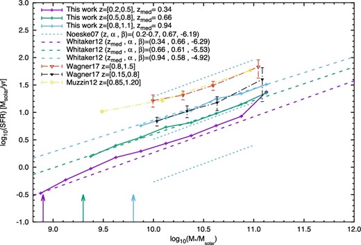
Median SFR of the SF main sequence in the field in redshift range of 0.2 < z < 0.5 (purple), 0.5 < z < 0.8 (green), and 0.8 < z < 1.1 (blue) from this work (solid lines) and from Whitaker et al. (2012) (dashed lines). The results of the SF main sequence in the field from Wagner et al. (2017) (red and black triangles), Muzzin et al. (2012) (yellow), and Noeske et al. (2007) with upper and lower limits (blue dotted lines) are also included For comparison. The purple, green, and blue arrows denote the mass completeness limit for SF galaxies at z = 0.5, 0.8, and 1.1. Our results, in general, are in agreement with the results from the literature. (Color online)
However, the SFRs of star-forming field galaxies from this study are lower than those from Wagner et al. (2017) and Muzzin et al. (2012) with a systematics offset ∼0.4 or 0.5 dex. The discrepancy from Wagner et al. (2017) could be larger since their SF main sequences is from SF cluster galaxies. The dissimilarity may come from the systematics between our samples. In Wagner et al. (2017), their galaxy sample consists of 25 clusters with 334 spectroscopic and 1975 photometric members over 0.15 < z < 1 from CLASH (Postman et al. 2012) and 11 clusters with 69 spectroscopic and 201 photometric members over 1 < z < 1.5 from ISCS (Eisenhardt et al. 2008). The estimation of SFRs and stellar masses for all galaxies is based on the SED fitting code, the Code Investigating GALaxy Emission code (Roehlly et al. 2014). In addition, they use the strength of the 4000 Å break Dn(4000) to divide the star-forming and quiescent populations, and their field contamination rate is ∼26%, and this may contribute to the main-sequence difference. Their redshift bin ranges, 0.15 < z < 0.8 and 0.8 < z < 1.5, are wider than our ranges, leading to the inclusion of higher-redshift galaxies and likely to higher median SFR in their results. On the other hand, Muzzin et al. (2012) have a redshift range similar to the high-redshift bin in this work, but the difference between their sample and ours is not easy to reconcile. However, their estimation of stellar mass and SFR is different from that which we employ.
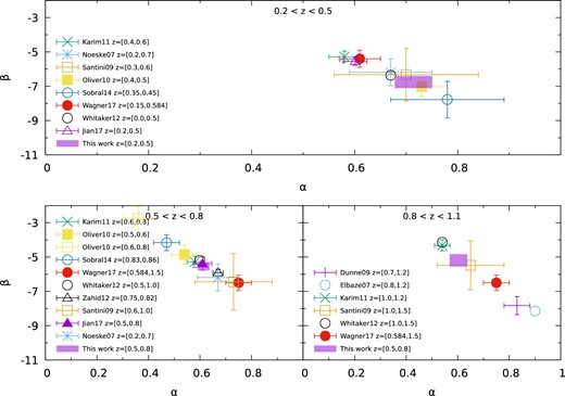
Best-fitting parameters α and β in equation (1) for SF galaxies are plotted in three redshift ranges. This figure is based on the work by Speagle et al. (2014), who compile and calibrate the best-fitting parameters from literature including Elbaz et al. (2007), Noeske et al. (2007), Dunne et al. (2009), Santini et al. (2009), Oliver et al. (2010), Karim et al. (2011), Whitaker et al. (2012), Zahid et al. (2012), and Sobral et al. (2014). Additionally, we add the results from Wagner et al. (2017), Jian et al. (2017) and this work. The best-fitting parameters from Whitaker et al. (2012) are without uncertainties and shown by open circles. (Color online)
3.2 Redshift dependence
3.2.1 sSFR of SF galaxies, sSFRSF(z)
There have been many previous studies to discuss and compare the evolution of the main sequence in different environments (Koyama et al. 2013; Lin et al. 2014; Erfanianfar et al. 2016; Wagner et al. 2017; Jian et al. 2017). Taking the advantage of the large and deep HSC sample, we are able to explore the same subject with better statistics and low-mass galaxies. In figure 5, the median sSFRs of the star-forming galaxies in field (dotted lines), group (dashed lines), and cluster (solid line) environments on the top, and the sSFR ratio of group to field galaxies (dashed lines) and that of cluster to field galaxies (solid lines) on the bottom are plotted as a function of redshift in different mass ranges separated into four panels. The yellow shaded region denotes the infrared main-sequence as defined in Elbaz et al. (2011) based on a Salpeter IMF, and is in the range of 13(13.8 Gyr − t)−2.2 < sSFR < 52(13.8 Gyr − t)−2.2, where t is the look-back time. The red data circles mark the sSFR of the star-forming galaxies in the field from Alberts et al. (2014) with stellar mass limit M > 1.3 × 10¹⁰ M⊙ and a Chabrier IMF assumed. Four cyan circles with error bars are from Wagner et al. (2017) for SF cluster galaxies of mass larger than log10(M*/M⊙) = 10.1. From figure 5, our results show good consistency with that in Elbaz et al. (2011) and slightly shallower at low z than that in Alberts et al. (2014). It is seen that the decrease of the sSFR of the SF main sequence for field galaxies is ∼0.45 dex from z = 1.1 to 0.2 for all mass bins, possibly due to a global decline in the gas contents. At fixed masses, the decrease level is very similar for cluster galaxies or group galaxies in different redshift ranges, and the reduction offset is seen <0.4 dex for clusters and <0.2 dex for groups. That is, the decrease of sSFRs for the group to field galaxies and for the cluster to field ones is independent of redshift. However, the decrease appears to depend on stellar mass, being larger for less-massive galaxies. Our results are in agreement with those in Koyama et al. (2013), that the difference in the SFR–M* relation between cluster and field SF galaxies is ∼0.2 dex since z ∼ 2.
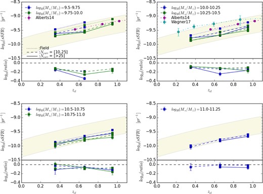
Top: Median sSFR of SF galaxies as a function of redshift in the field (dotted), groups (dashed), and clusters (solid). Bottom: The logarithmic ratio of sSFR for group to field galaxies (dashed), and for cluster to field galaxies (solid). In addition, the red and cyan circles denote the sSFR of SF galaxies in the field from Alberts et al. (2014) for M* > 1.3 × 10¹⁰ M⊙ and in clusters from Wagner et al. (2017) for M* > 1010.1 M⊙, respectively. The yellow shaded region shows the boundaries of the infrared main sequence as defined in Elbaz et al. (2011). In the upper left-hand panel, the data points in the redshift range of 0.8 < z < 1.1 for the mass bin 9.5–9.75 are removed due to the mass incompleteness. The trend that the sSFR decreases with the decreasing redshift and the decreasing level for the same redshift range in our results are in good agreement with other works, although a systematics is seen. (Color online)
3.2.2 Quiescent fraction, fq(z)
Under the stellar mass control, the redshift dependence of the quiescent fractions (fq) for field (dotted lines), group (dashed lines), and cluster (solid lines) galaxies is explored in figure 6. For comparison, the results from Wagner et al. (2017) (cyan circles) with M* > 1010.1 M⊙ are also plotted in figure 6. Globally, the fq increases with decreasing redshift, consistent with the Butcher–Oemler effect (Butcher & Oemler 1984). However, depending on the galaxy masses, their effect can be significantly different. For high-mass galaxies, the Butcher–Oemler effect is weak and nearly negligible. On the other hand, the effect is stronger for low-mass galaxies, consistent with results in Li et al. (2012). For low-mass galaxies, the increase of fq is about 3 times larger from high z, ∼0.95 to low z, ∼0.35. In addition, the cluster downsizing effect, where clusters with larger halo mass show a greater quiescent fraction, is also evident in our sample. Our redshift evolution trend is similar to that in Wagner et al. (2017), and the fq derived for our sample in log10(M*/M⊙) = 10.2–10.5 (the blue solid line in the upper right-hand panel) also appears to be consistent with those in Wagner et al. (2017).
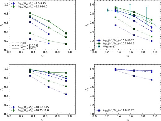
Redshift evolution of the quiescent fractions (fq) for field (dotted), group (dashed), and cluster (solid) galaxies. Similar to the upper left-hand panel in figure 5, the data points in the high-redshift bin for the mass bin 9.25–9.5 are removed due to the mass incompleteness. The Butcher–Oemler effect (Butcher & Oemler 1984) is clearly seen but with a mass dependence. The effect is stronger for less-massive galaxies and lesser for massive galaxies. For comparison, we also add the fq results from Wagner et al. (2017) (cyan circles) with M* > 1010.1 M⊙ in the upper right-hand panel. It is seen that our result is in agreement with that from Wagner et al. (2017). (Color online)
3.2.3 Quenching efficiency, ε(z)
We also compute the environmental quenching efficiency, |$\varepsilon ^{{\rm envi}} = (f^{{\rm cluster}}_{\rm q} - f^{{\rm field}}_{\rm q})/(1 - f^{{\rm field}}_{\rm q})$|, similar to the definition in (Peng et al. 2010), as a function of redshift in different mass bins in order to quantify the excess of quenching due to pure environmental effects in figure 7. For comparison, environmental quenching efficiencies estimated from other studies of groups and clusters at various redshifts compiled by Nantais et al. (2016) are plotted. The data points include results from Balogh et al. (2016) for M* > 1010.3 M⊙ in redshift range 0.8 < z < 1.2, van der Burg et al. (2013) for M* > 1010.0 M⊙ redshift range 0.86 < z < 1.34, Kawinwanichakij et al. (2016) for 109.3 < M* < 1010.2 M⊙ in redshift range 0.3 < z < 2.5, Knobel et al. (2013) for M* ∼ 1010.65 M⊙ in redshift range 0.1 < z < 0.8, van den Bosch et al. (2008) for M* ∼ 109 M⊙ in redshift range 0.01 < z < 0.2, Omand, Balogh, and Poggianti (2014) for M* > 1010 M⊙ in redshift range 0.01 < z < 0.2, Cooke et al. (2016) for M* > 1010.5 M⊙ at redshift z ∼ 1.58, Quadri et al. (2012) for 1010.3 < M* < 1010.6 M⊙ in redshift range 0.5 < z < 1.5, and Nantais et al. (2016) for M* > 1010.1 M⊙ in redshift range 1.37 < z < 1.63. In general, our results show consistency with other people’s work. However, a stronger redshift evolution trend in the quenching efficiency is observed in our data than that from the literature. It is seen that the quenching efficiency increases with the decreasing redshift, and also increases with the increasing mass at fixed redshift. However, the slope of the quenching efficiency decreases with the increasing masses, implying that the evolution of the quenching effect is stronger for less-massive galaxies. The redshift dependence becomes weaker for the high-mass galaxies, likely due to being red and dead already for most of the massive galaxies at high redshifts. In addition, it is seen that the environmental quenching in clusters is larger than that in groups, indicating that the hosting environment has a significant effect on the star formation quenching, in agreement with results from the literature cited previously.
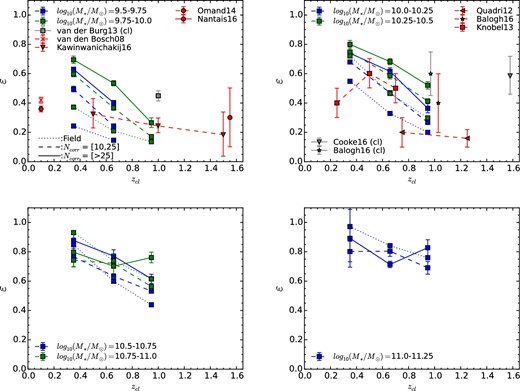
Similar to figures 5 and 6, the quenching efficiency ε is plotted as a function of redshift for different mass ranges in four panels for field (dotted), group (dashed), and cluster (solid) galaxies, respectively. In general, the slope of the quenching efficiency decreases with the increasing masses, implying that the quenching effect is stronger for less-massive galaxies. (Color online)
3.3 Stellar mass dependence
3.3.1 sSRF of SF galaxies, sSFRSF(M*)
In figure 8, the sSFRs of SF galaxies are plotted as a function of the stellar mass M* in different hosting environments and redshift ranges. In the upper left-hand panel, the median sSFR of SF field galaxies is shown in the redshift ranges of 0.2 < z < 0.5 (dashed line), 0.5 < z < 0.8 (solid line), and 0.8 < z < 1.1 (dotted line) for comparison. For the other three panels on the top right, bottom left, and bottom right, the sSFRs of SF field (black pluses), group (blue squares), and cluster (green circles) galaxies are plotted on the top while the logarithmic ratio of sSFR for SF group to field galaxies (blue squares) and that for SF cluster to field ones (green circles) are displayed on the bottom. Additionally, the red pluses, squares, and circles denote the sSFR of SF field, group, and cluster galaxies in 0.5 < z < 0.8 from Lin et al. (2014), respectively. The cyan circles are the sSFRs of SF cluster galaxies in 0.15 < z < 0.8 and in 0.8 < z < 1.5 from Wagner et al. (2017), and the purple pluses and circles are those of SF field and cluster galaxies in 0.85 < z < 1.2 from Muzzin et al. (2012).
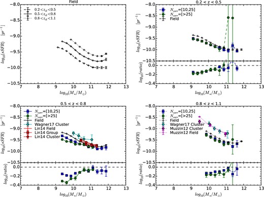
Similar to figure 5, but the sSFRs of SF galaxies are shown as a function of stellar mass. In the upper left-hand panel, the sSFR of SF field galaxies in redshift ranges of 0.2 < z < 0.5, 0.5 < z < 0.8, and 0.8 < z < 1.1 is represented by the dashed, solid, and dotted lines, respectively. The other three panels plot the sSFRs of SF field (black pluses), group (blue squares), and cluster (green circles) galaxies on the top, and the logarithmic ratio of sSFR for group to field galaxies (blue squares), and for cluster to field galaxies (green circles), on the bottom. For comparison, we also include the sSFR results from Lin et al. (2014) in the redshift range of 0.5 < z < 0.8 for SF field (red pluses), group (red squares), and cluster (red circles) galaxies. In addition, the sSFR results are added as well from Muzzin et al. (2012) for SF field (purple pluses) and cluster (purple circles) galaxies in the redshift range 0.85 < z < 1.2, and from Wagner et al. (2017) for SF cluster galaxies (cyan circles) in the redshift ranges of 0.15 < z < 0.8 (bottom left) and 0.8 < z < 1.5 (bottom right). (Color online)
In general, the sSFR of cluster and field galaxies decreases with the increasing mass, and the decreasing trend is in broad agreement with that in Vulcani et al. (2010) and Haines et al. (2013). In addition, we found that there is a weak dependence on the stellar mass of the sSFR deficit relative to the field, which is <0.2 dex in groups and <0.4 dex in clusters, consistent with results found in Haines et al. (2013) that the sSFRs of star-forming cluster galaxies (M > 1010 M⊙) are systematically ∼28% lower than those in the field at fixed stellar mass in 0.15 < z < 0.3. The decrease of the sSFR in group or cluster galaxies from that in field ones suggests that a slow quenching effect likely acts in dense environments. The larger deficit seen in cluster galaxies as opposed to group galaxies also suggests a stronger environmental quenching effect in clusters than in groups. It is worth noting that the decreases are slightly larger from what was found in Lin et al. (2014), who found no significant sSFR reduction of SF galaxies in the groups and ∼17% (0.23 dex) sSFR decrease for the SF galaxies in the clusters relative to the field galaxies. However, we note that the halo mass binning is 1013.6–14.2 M⊙ for groups and 10>14.2 M⊙ for clusters in this work while it is 1013.4–14.0 M⊙ for groups and 10>14.0 M⊙ for clusters in Lin et al. (2014). The larger sSFR offset seen in this work may be attributed to the greater mass of the groups and clusters probed in our analysis, since larger sSFR reduction is expected in more-massive clusters. In addition, less-massive groups normally suffer from the more serious foreground and background contaminations and the real group signals can be easily smeared out, leading to the less sSFR reduction than from the sample without the field contamination. In the high-redshift (bottom-right) panel, although there seems to have a systematic between our results and the results from Muzzin et al. (2012) and Wagner et al. (2017) for the absolute sSFR values, the decreasing trend of the sSFR with the increasing mass in our sample agrees well with them. Besides, it is noticed that our results for the sSFR reductions are in broad agreement with those from Muzzin et al. (2012).
3.3.2 Quiescent fraction, fq (M*)
The quiescent fraction (fq) is investigated as a function of M* in figure 9. Similar to figure 8, the upper-left-hand panel shows the fq for field galaxies in three redshift ranges, and the other three panels give the comparisons of fq for the field, group, and cluster galaxies in one redshift range per panel. Results of fq are included For comparison from Muzzin et al. (2012) for field and cluster galaxies in the redshift range of 0.85 < z < 1.2, from Lin et al. (2014) for field, group, and cluster galaxies in 0.5 < z < 0.8, and from Wagner et al. (2017) for cluster galaxies in 0.15 < z < 0.41, 0.41 < z < 0.8, and 0.8 < z < 1.5. It is seen that the quiescent fraction depends strongly on mass and less strongly on redshift and the hosting environment. At high redshifts, the fq difference at fixed mass between group and cluster galaxies is small and gradually becomes larger with the decreasing redshift, indicating that the environmental quenching effect has a redshift dependence. In addition, the typical “downsizing” effect in which less-massive galaxies are more star-forming continues down to ∼109 M⊙. Moreover, at low mass, it is found that the red sequence is still visible in groups or clusters with respective to the field, implying that the environmental quenching can still effectively stop star formation for low-mass galaxies. It is noticed that the fq in this work is higher compared to those from Lin et al. (2014) and Wagner et al. (2017). Besides the greater cluster masses used in this work (see the discussion in sub-subsection 3.3.1), it is also likely that the CAMIRA cluster finding is based on the red sequence method and preferentially selects clusters with high fq. In the high-redshift range, our fq values broadly agree with those from Muzzin et al. (2012). However, lower fq values are found in Wagner et al. (2017), likely due to the fact that their sample includes galaxies up to z ∼ 1.5.
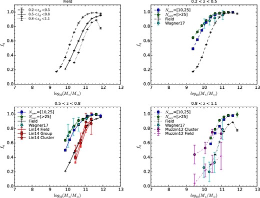
Quiescent fraction fq values as a function of stellar mass. In the upper left-hand panel, the fq values are plotted for field galaxies in three redshift bins while the other three panels show the fq values of field (black pluses), group (blue squares), and cluster (green circles) galaxies in redshift range of 0.2 < z < 0.5 (upper right), 0.5 < z < 0.8 (bottom left), and 0.8 < z < 1.1 (bottom right). The red pluses, squares, and circles denote the fq values for field, group, and cluster galaxies, respectively, from Lin et al. (2014) in redshift range of 0.5 < z < 0.8. The cyan circles are data points from Wagner et al. (2017) for cluster galaxies in redshift range of 0.15 < z < 0.41 (upper right), 0.41 < z < 0.8 (bottom left) and 0.8 < z < 1.5 (bottom right). The purple pluses and circles represent the fq values for field and cluster galaxies, respectively, from Muzzin et al. (2012) in the redshift range of 0.85 < z < 1.2. (Color online)
3.3.3 Quenching efficiency, ε(M*)
The environmental quenching efficiency is shown as a function of stellar mass in figure 10 in order to better quantify the excess of quenching due to pure environmental effects. The panel arrangement is similar to that in figures 8 and 9. In the upper left-hand panel, the quenching efficiency from field galaxies, or the mass quenching efficiency assuming that field galaxies are purely quenched by their masses, are displayed in three redshift ranges. The other three panels present the comparisons among the field, group, and cluster galaxies per redshift bin. It is clearly seen that both the mass and environmental quenching increases with increasing stellar mass. However, high-mass galaxies are dominated by the mass quenching while low-mass galaxies are quenched primarily due to the environmental quenching. The transition mass, where the dominance of the mass and environmental quenching switches, is recognized at log10(M*/M⊙) ∼ 10.4 in groups and 10.6 in clusters in the lowest redshift range of 0.2 < z < 0.5, in good agreement with the results from Lin et al. (2014). This implies that the environmental quenching in clusters is more prominent than that in groups since it can quench more massive galaxies than in groups.
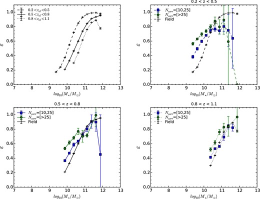
Quenching efficiency ε values as a function of stellar mass. Similar to figures 8 and 9, the ε values of field galaxies in three redshift bins are shown in the upper left-hand panel while the other three panels plot the ε values of field (black pluses), group (blue squares), and cluster galaxies (green circles) in three redshift ranges, respectively. It is clearly seen that the transition masses from the dominance of the environment quenching to that of the mass quenching are log10(M*/M⊙) ∼ 10.4 in groups and ∼10.6 in clusters. (Color online)
4 Conclusion and discussion
In this work, we probe galaxies down to i ∼ 26, two magnitudes deeper than that in our previous works (Lin et al. 2014; Jian et al. 2017), and extend our results to redshift 1.1, enabling us to study the cosmic evolution of the star formation activity. Due to the exceptional deep depth of our sample, the stellar mass completeness limit can be pushed to log10(M*/M⊙) = 9.8 and 10.3 at z ∼ 1.1 for star-forming and quiescent galaxies, respectively. That is, we are able to explore the quenching status of lower-mass star-forming galaxies which have not been explored in our previous works. Additionally, the HSC Wide 16A data are collected from a survey area of ∼174 square degree to offer good statistics even for galaxies at the high-mass end. In other words, we can constrain the results on high-mass galaxies more robustly as opposed to previous studies. The main results can be summarized below:
1. The sSFR of star-forming galaxies decreases with cosmic time, regardless of the environment. The sSFR is lower in groups and clusters than in the field by ∼0.1 dex and ∼0.2–0.3 dex, respectively. The drop of sSFR in group/cluster environments is insensitive to the redshift and is more significant for low-mass galaxies.
2. The quiescent fraction is a strong function of stellar mass in all environments, being greater for higher-mass galaxies. The Butcher–Oemler effects are seen in all environments and are more prominent for low-mass galaxies.
3. Both the environment and stellar mass quenching efficiencies increase with the stellar mass. However, the environment quenching dominates over the stellar mass quenching for low-mass galaxies.
At a fixed stellar mass, we find that the decrease in the sSFR of star-forming group or cluster galaxies to field ones is 0.1–0.3 dex and is more prominent in cluster environments. This implies that galaxies in clusters likely experience a long timescale (or slow) quenching effect that gradually reduces the SFR of star-forming galaxies. Although the gas contents and hence the star formation rate of galaxies vary with redshifts, we find that the offsets in the sSFR in groups/clusters, as opposed to the field, are comparable at different redshifts, in agreement with the results found by Koyama et al. (2013). This implies that the slow quenching mechanism acting on groups/clusters is likely universal in the redshift range of 0.2 < z < 1.1.
In addition, it is found in this work that the transition masses from environment quenching to the mass quenching are 1010.4 M⊙ and 1010.6 M⊙ in groups and clusters, respectively, in the lowest redshift bin of 0.2 < z < 0.5, in good agreement with the results from Lin et al. (2014). The greater transition mass in clusters suggests that the environment effects are more important in clusters than in groups and have an effect even for massive galaxies. It is also noticed that the red fraction for the most massive galaxies is comparable between the field and group/cluster environments. This suggests that the star formation of those massive galaxies beyond the transition mass are likely already stopped and are red and dead before they enter the cluster-like environments. Conversely, the environmental quenching dominates the mass quenching in low-mass galaxies below the transition mass in groups or clusters down to the mass completeness limit of 108.6 M⊙ at z ∼ 0.2, and the environmental quenching effect in clusters is stronger than that in groups. At this low-mass regime, the red sequence is still visible in groups or clusters with respect to the field, suggesting that the environmental quenching can still effectively stop star-formation for low-mass galaxies.
Koyama et al. (2018) recently presented their results discussing the environmental dependence of color, stellar mass, and sSFR of Hα-selected galaxies in twin clusters in the DEEP2-3 field at z = 0.4. One important finding in their work is that H-selected galaxies reveal color–density or color–radius correlations, but their stellar masses or sSFRs are independent of environments. The conclusion appears to be inconsistent with our result that there is a systematical reduction of sSFR for SF galaxies in groups or clusters by 0.1–0.3 dex with respect to those in the field. As discussed in Koyama et al. (2018), there are various factors that may contribute to this discrepancy. It is likely due to different definitions for SF galaxies in our and their sample. Our SF galaxies are determined by their sSFRs while SF galaxies are detected as Hα galaxies in Koyama et al. (2018). In addition, it is indicated that the treatment of dust extinction or N ii line contamination could easily change the results by >10%–20%, which can significantly ease the inconsistency between our result and the result from Koyama et al. (2018). Finally, it is also possible that the sample size of Hα emitters in Koyama et al. (2018) is much smaller than that of our sample, which covers whole HSC S16A Wide survey area, and poor statistics (particularly in a high-density environment) may lead to the disagreement in conclusions.
Acknowledgements
This work is supported by the Ministry of Science & Technology of Taiwan under the grant MOST 103-2112-M-001-031-MY3 and MO is supported in part by World Premier International Research Center Initiative (WPI Initiative), MEXT, Japan, and JSPS KAKENHI Grant Number 26800093 and 15H05892. The Hyper Suprime-Cam (HSC) collaboration includes the astronomical communities of Japan and Taiwan, and Princeton University. The HSC instrumentation and software were developed by the National Astronomical Observatory of Japan (NAOJ), the Kavli Institute for the Physics and Mathematics of the Universe (Kavli IPMU), the University of Tokyo, the High Energy Accelerator Research Organization (KEK), the Academia Sinica Institute for Astronomy and Astrophysics in Taiwan (ASIAA), and Princeton University. Funding was contributed by the FIRST program from Japanese Cabinet Office, the Ministry of Education, Culture, Sports, Science and Technology (MEXT), the Japan Society for the Promotion of Science (JSPS), Japan Science and Technology Agency (JST), the Toray Science Foundation, NAOJ, Kavli IPMU, KEK, ASIAA, and Princeton University.
References
