


Abstract
Centaurs have orbits between Jupiter and Neptune and are thought to originate from the trans-Neptunian region. Observations of surface properties of Centaurs and comparison with those of trans-Neptunian objects (TNOs) would provide constraints on their origin and evolution. We analyzed imaging data of nine known Centaurs observed by the Hyper Suprime-Cam (HSC) installed on the Subaru Telescope with the g- and i-band filters. Using the data available in the public HSC data archive, as well as those obtained by the HSC Subaru Strategic Program (HSC-SSP) by the end of 2017 June, we obtained the g − i colors of the nine Centaurs. We compared them with those of known TNOs in the HSC-SSP data obtained by T. Terai et al. (2018, PASJ, 70, S40). We found that the color distribution of the nine Centaurs is similar to that of those TNOs with high orbital inclinations, but distinct from those TNOs with low orbital inclinations. We also examined correlations between the colors of these Centaurs and their orbital elements and absolute magnitude. The Centaurs’ colors show a moderate positive correlation with semi-major axis, while no significant correlations between the color and other orbital elements or absolute magnitude were found for these Centaurs. On the other hand, recent studies on Centaurs with larger samples show interesting correlations between their color and absolute magnitude or orbital inclination. We discuss how our data fit in these previous studies, and also discuss implications of these results for their origin and evolution.
1 Introduction
Recent models of planet formation show that giant planets in the solar system likely experienced significant radial migration, causing dramatic influence on nearby small bodies (Tsiganis et al. 2005; Walsh et al. 2011). Numerical simulations show that scattering by the migrating giant planets in the presence of the nebular gas can explain the degree of radial mixing in the present asteroid belt (Walsh et al. 2011). Migration of the giant planets after their formation and the dispersal of the nebular gas leads to injection of a large number of small icy bodies originally in the trans-Neptunian disk into planet-crossing orbits. Some of these objects were presumably captured as Jupiter’s Trojan asteroids (Morbidelli et al. 2005; Nesvorný et al. 2013), while others were further delivered into the asteroid belt (Levison et al. 2009) or even into the terrestrial region (Gomes et al. 2005). The transfer of small bodies from the trans-Neptunian region to planet-crossing orbits has continued after planet formation, and some of them are observed today as Centaurs. Therefore, observational studies of trans-Neptunian objects (TNOs), Centaurs, and other small solar system bodies can provide us with important information about the evolution of the solar system.
Spectroscopic studies of small bodies give us detailed information about their surface properties and composition. However, obtaining such data for a large number of distant small bodies is a difficult and telescope-time-consuming task. On the other hand, photometric observation using multiple broadband filters allows us to perform a statistical study of a large number of objects, including rather faint ones (see reviews by Doressoundiram et al. 2008; Tegler et al. 2008). Using these data, we can obtain the color distribution of small-body populations, which can be used to infer their origin and evolution. So far, more than 2000 TNOs have been found. Colors of TNOs have been measured and correlations with orbital elements and other quantities have been extensively studied (for a review, see Doressoundiram et al. 2008). These studies show that a group of TNOs with low orbital eccentricity/inclination (often called cold classical Kuiper-belt objects) tend to be significantly redder than other TNOs (e.g., Tegler & Romanishin 1998; Tegler et al. 2016), while those in other groups seem to have similar color distributions. The size distribution of the cold classical TNOs is also distinct from other TNOs (Fraser et al. 2014). These pieces of observational evidence suggest that the cold TNOs likely formed approximately where they are today, in contrast to those TNOs in other dynamical groups, which are thought to have experienced significant scattering and radial mixing due to perturbations by the giant planets. Also, it has been shown that small TNOs have a bimodal color distribution (Peixinho et al. 2012, 2015; Tegler et al. 2016; Wong & Brown 2017), which are often called gray and red groups (These are called red and very red color groups in Wong & Brown 2017). On the other hand, Jupiter’s Trojan asteroids form a group of small bodies with the largest number of confirmed members (>7000) in the outer solar system. The overall color distribution of Jupiter Trojans is roughly similar to the gray group of TNOs, but it shows bimodality for sub-groups within the Trojan population (Emery et al. 2011; Wong et al. 2014). Wong and Brown (2016) proposed a model for the origin and evolution of the two Trojan color sub-populations based on the depletion or retention of H2S ice on their surface.
Centaurs are small solar system bodies located between the orbits of Jupiter and Neptune, and more than 400 bodies with confirmed orbits are listed in the JPL database. It should be noted that there are some variations in the definition of Centaurs. For example, the JPL database defines Centaurs as objects with 5.5 au < a < 30.1 au (a is the object’s semi-major axis), with the outer boundary corresponding to Neptune’s semi-major axis aN, while q = 5.2 au (q is the perihelion distance) is used for the inner boundary in the Minor Planet Center database. Furthermore, Gladman, Marsden, and Vanlaerhoven (2008) proposed to adopt TJ = 3.05 (TJ being the Tisserand parameter with respect to Jupiter) and q = 7.35 au as the inner boundary, i.e., the boundary between Centaurs and Jupiter-family comets. Centaurs are likely delivered from the trans-Neptunian disk by planetary perturbations (Levison & Duncan 1997), but their origin is not well understood. Owing to perturbations by the giant planets, Centaurs’ dynamical lifetime is rather short (∼106 yr; Tiscareno & Malhotra 2003; Horner et al. 2004). Some Centaurs may evolve to become Jupiter-family comets, but eventually these objects will be ejected from the solar system or collide with one of the planets (Tiscareno & Malhotra 2003). Therefore, studies on the origin of Centaurs allow us to better understand the process of delivery of small icy bodies from the trans-Neptunian region as well as the origin of Jupiter-family comets.
Survey observations estimate that there are about 107 Centaurs with diameter D > 2 km and 100 with D > 100 km (Sheppard et al. 2000). The total mass of Centaurs is estimated to be about 10−4 M⊕, which is as large as one tenth of the total mass of the main-belt asteroids. Spectral observations have revealed that some Centaurs show signatures of various ices (Barucci et al. 2008), but most of the information on their surface properties comes from photometric observations (Hainaut & Delsanti 2002; Tegler et al. 2008, 2016; Hainaut et al. 2012). A notable characteristic of Centaurs’ color distribution is that it is bimodal, with gray and red groups (Peixinho et al. 2003; Tegler et al. 2003). Recent studies show that the bimodal color distribution is common to both Centaurs and small TNOs (Peixinho et al. 2012, 2015; Tegler et al. 2016; Wong & Brown 2017). However, the available color data for Centaurs is still limited at present. So, for an improved statistical study of color distribution and correlations between colors and other quantities (e.g., orbital elements), increasing the number of data with good quality is essential. Also, a comparison of colors using a uniform set of data obtained by the same instrument for objects in different dynamical groups can improve the quality of the comparison.
In the present work, we obtain the color distribution of nine Centaurs observed by the Hyper Suprime-Cam (HSC) installed on the Subaru Telescope. We examine correlations between colors and other quantities, i.e., orbital elements and absolute magnitude. We compare the obtained color distribution with that of known TNOs obtained by HSC (Terai et al. 2018). The HSC data used in this work and that of Terai et al. (2018) are of optimal quality and obtained by the same survey/instrument. On the other hand, recent studies on Centaurs with larger samples demonstrate interesting correlations between their color and other quantities, such as absolute magnitude (Peixinho et al. 2012; Tegler et al. 2016), and we will discuss how our data fit with these recent studies. Based on these results, we discuss implications for the origin and evolution of Centaurs. We describe the data used in the present work in section 2. The results of our data analysis are presented in section 3, and we discuss and summarize our results in section 4.
2 Data
2.1 Observation and object sample
We use imaging data obtained by the HSC. The HSC is a prime focus camera for the 8.2 m Subaru Telescope, and consists of 116 2048 × 4096 pixel CCDs (104 for science, 8 for focus monitoring, and 4 for auto guiding). It has a field of view |${1{^{\circ}_{.}}5}$| in diameter with a pixel scale of |${0{^{\prime\prime}_{.}}168}$| (Miyazaki et al. 2012). The data we used in the present work are those obtained through the HSC Subaru Strategic Program (HSC-SSP) by the end of 2017 June, as well as those available in the public HSC data archive, which were obtained by the end of March 2016. The HSC-SSP project is a multi-band imaging survey with g, r, i, |$z$|, Y broad-band and four narrow-band filters, covering ∼1400 deg2 of the sky for 300 nights over 5–6 yr from 2014 March (Aihara et al. 2018). As we describe below, we use data taken with the g- and i-band filters.
In the present work, we perform photometric investigations of known Centaurs using the above HSC data. The daily ephemeris of each known Centaur was retrieved from the Minor Planet & Comet Ephemeris Service website managed by the Minor Planet Center. We searched for known Centaurs with coordinates located within the area of the HSC data mentioned above at their acquisition dates, and checked if there was a detected source corresponding to each of those objects in the source catalogs using the sub-hourly ephemeris. The identified source was checked by visual inspection. If the source was judged not to be an actual Centaur (e.g., a star, galaxy, or artifact) or its image had any problems (e.g., located at the edge of the image or too close to a very bright object), it was excluded from our analysis. We selected objects observed in both the g and i bands as the targets of this study, since previous works show that the g − i color is a useful indicator to distinguish populations of small bodies in the outer solar system (Wong & Brown 2016, 2017; Terai et al. 2018). Based on the above criteria we finally found nine Centaurs suitable for the present study. Table 1 provides a list of these objects and their acquisition dates in each band. For those objects observed multiple times with the same filter during one night, the average time interval for observations was about 11 min.
Measured Centaurs and their acquisition dates for each filter.*
| Object | Filter | UT date |
|---|---|---|
| 1977 UB (Chiron) | g | 2015-10-14 (1), 2016-08-28 (5) |
| i | 2016-09-05 (1) | |
| 1998 QM107 (Pelion) | g | 2015-10-07 (10), 2017-01-26 (1) |
| i | 2015-10-07 (11) | |
| 2006 SX368 | g | 2014-11-20 (4) |
| i | 2014-11-19 (4) | |
| 2012 DD86 | g | 2015-03-25 (4), 2016-04-04 (6), 2016-04-05 (2), 2016-04-06 (3), |
| 2017-03-05 (1), 2017-03-29 (1) | ||
| i | 2015-03-20 (4), 2016-04-02 (4), 2017-04-27 (3) | |
| 2013 RG98 | g | 2015-01-20 (5) |
| i | 2015-01-17 (5) | |
| 2014 AT28 | g | 2015-10-14 (1) |
| i | 2014-09-24 (9) | |
| 2014 GP53 | g | 2015-03-25 (5), 2016-04-04 (1) |
| i | 2014-03-28 (4), 2015-03-20 (5), 2015-03-22 (1), 2016-04-09 (2) | |
| 2014 SR303 | g | 2014-07-06 (4), 2014-09-23 (2) |
| i | 2014-07-08 (7), 2014-09-23 (1) | |
| 2015 DB216 | g | 2016-01-11 (5) |
| i | 2016-01-12 (6) |
*The number of data points for each date is displayed in parentheses.
Figure 1 shows the semi-major axes and eccentricities of the above nine Centaurs (see also table 2). The vertical straight line at a = 30.1 au shows the outer boundary commonly used in various definitions of Centaurs (section 1). We show three examples of the inner boundary in figure 1: a = 5.5 au (JPL database), q = 5.2 au (MPC), and q = 7.35 au (Gladman et al. 2008). Most of the objects are not affected by the choice of the inner boundary. However, the one near the inner boundary (2014 AT28) is included as a Centaur in JPL’s and MPC’s definitions, while it is excluded in the definition of Gladman, Marsden, and Vanlaerhoven (2008). It should also be noted that this object is on a retrograde orbit about the Sun (table 2), and thus it likely experienced dynamical evolution that is quite different from other objects (Brasser et al. 2012; Volk & Malhotra 2013). Therefore, although we will measure its color together with the other eight Centaurs, we will exclude this object when we perform statistical analysis for correlations of the obtained color distribution with orbital elements and absolute magnitude (subsection 3.2).
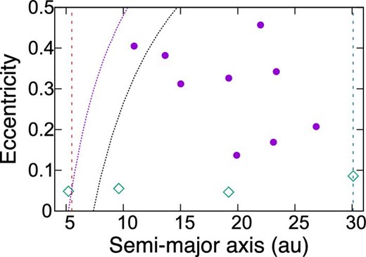
Distribution of the semi-major axes and eccentricities of the nine Centaurs examined in the present work (circles). The diamonds represent the four giant planets for comparison. The two vertical dashed lines represent a = 5.5 au and a = aN (aN is Neptune’s semi-major axis), respectively. The two dotted curves represent q = 5.2 au and q = 7.35 au, respectively. (Color online)
Orbital elements, absolute magnitudes, and g − i colors of Centaurs.*
| Object | a (au) | q (au) | e | I (°) | Hg (mag) | Hi (mag) | g − i (mag) |
|---|---|---|---|---|---|---|---|
| 1977 UB (Chiron) | 13.648 | 8.431 | 0.382 | 6.950 | 5.92 ± 0.01 | 4.97 ± 0.01 | 0.95 ± 0.09 |
| 1998 M107 (Pelion) | 19.911 | 17.178 | 0.137 | 9.348 | 10.47 ± 0.10 | 9.65 ± 0.04 | 0.82 ± 0.17 |
| 2006 SX368 | 21.997 | 11.945 | 0.457 | 36.325 | 9.95 ± 0.00 | 8.84 ± 0.01 | 1.11 ± 0.18 |
| 2012 DD86 | 23.373 | 15.372 | 0.342 | 12.498 | 9.91 ± 0.04 | 8.52 ± 0.03 | 1.40 ± 0.07 |
| 2013 RG98 | 23.125 | 19.224 | 0.169 | 46.036 | 9.55 ± 0.02 | 8.21 ± 0.03 | 1.34 ± 0.17 |
| 2014 GP53 | 26.860 | 21.308 | 0.207 | 14.256 | 9.75 ± 0.04 | 7.83 ± 0.01 | 1.92 ± 0.08 |
| 2014 SR303 | 15.017 | 10.333 | 0.312 | 3.035 | 11.62 ± 0.02 | 10.41 ± 0.02 | 1.21 ± 0.06 |
| 2014 AT28 | 10.942 | 6.512 | 0.405 | 165.559 | 12.84 ± 0.00 | 11.16 ± 0.01 | 1.69 ± 0.16 |
| 2015 DB216 | 19.211 | 12.944 | 0.326 | 37.701 | 8.91 ± 0.00 | 7.65 ± 0.01 | 1.26 ± 0.18 |
*Semi-major axis (a), perihelion distance (q), eccentricity (e), inclination (I), measured absolute magnitudes in the g and i bands (Hg and Hi), and the g − i color. Note that 2014 AT28 has a retrograde orbit.
2.2 Data reduction and color measurement
The procedures for data reduction and analysis adopted in the present work are similar to those in Terai et al. (2018). The data were processed with hscPipe, which is the HSC data reduction/analysis pipeline developed by the HSC collaboration team (Bosch et al. 2018) based on the Large Synoptic Survey Telescope (LSST) pipeline software (Ivezic et al. 2008; Axelrod et al. 2010; Jurić et al. 2015). First, a raw image is reduced by CCD-by-CCD procedures including bias subtraction, linearity correction, flat fielding, artifacts masking, and background subtraction. Next, the pipeline detects sources and determines the World Coordinate System (WCS) and zero-point magnitude of the corrected data by matching to the Pan-STARRS 1 (PS1) 3π catalog (Tonry et al. 2012; Schlafly et al. 2012; Magnier et al. 2013). Then, centroids, shapes, and fluxes of the detected sources are measured with several different algorithms. We use the sinc aperture flux (Bickerton & Lupton 2013) with a 12 pixel (i.e., ∼|${2.^{\prime \prime }}0$|) radius aperture for photometry of the detected objects, which is also used in the estimate of the zero-point magnitude. Note that the zero points are translated from PS1 into the native HSC system by a color term (Kawanomoto et al. 2018). Finally, the pipeline generates source catalogs of measured values and flags for detected objects in each CCD.
In addition to the photometric error, brightness variation due to the small body’s rotation also contributes to uncertainty in the color measurement. According to the analysis by Duffard et al. (2009), the mean rotation period and lightcurve amplitude of Centaurs are 6.75 hr and 0.26 mag, respectively. Using a Monte Carlo method, we generated synthetic lightcurves assuming a sinusoidal brightness fluctuation with 6.75 hr period, 0.26 mag amplitude, and random initial phase angles at the actual acquisition epochs of each object/band. The error in color caused by rotation is evaluated by the standard deviation (σrot) of the color offsets. The typical value is σrot ∼ 0.1 mag. Finally, the total color uncertainty is estimated from |$\sqrt{ \sigma _{H_g}^2 + \sigma _{H_i}^2 + \sigma _{\rm rot}^2 }$|.
The averaged absolute magnitudes (Hg and Hi) and g − i colors obtained for all the sample objects are shown in table 2. Note that the magnitudes and colors are expressed in the Vega magnitude system hereafter.
3 Results
3.1 Color distribution
The color distribution of the nine Centaurs obtained in the present work is shown in the top panel of figure 2. The solar color is given by Holmberg, Flynn, and Portinari (2006), and is converted into the HSC band system with color term correction (see table 3 of Terai et al. 2018). Here, we use g − i = 1.02 mag, which is shown with the dashed line for comparison in figure 2. We find that the colors of the nine Centaurs are distributed over the range from neutral to slightly red colors. The g − i color of Chiron obtained by the present work was about 0.96 mag, which is consistent with previous works (Hartmann et al. 1990; Meech & Belton 1990; Luu & Jewitt 1990; Hainaut & Delsanti 2002; Romon-Martin et al. 2003). We do not see the clear bimodality in the color distribution that was found in previous works (Tegler & Romanishin 2003; Peixinho et al. 2003; Tegler et al. 2003; see a review by Tegler et al. 2008), owing to the small number of objects examined in the present work; comparison with previous works with larger samples will be discussed in subsection 3.2.
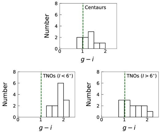
Top panel: Distribution of g − i color of the nine Centaurs examined in the present work. The vertical dashed line represents the solar color (g − i = 1.02). Bottom panels: Distributions of g − i color of TNOs examined by Terai et al. (2018) based on the HSC-SSP data. The left panel shows the distribution of 13 objects with low inclination (I < 6°), and the right panel shows that of 13 objects with high inclination (I > 6°). Data for the bottom panels were taken from Terai et al. (2018). (Color online)
Results of correlation test.*
| a | q | e | I | Hi | |
|---|---|---|---|---|---|
| r s | 0.738 | 0.571 | −0.095 | 0.429 | −0.238 |
| Pt | 0.037 | 0.139 | 0.823 | 0.289 | 0.570 |
| a | q | e | I | Hi | |
|---|---|---|---|---|---|
| r s | 0.738 | 0.571 | −0.095 | 0.429 | −0.238 |
| Pt | 0.037 | 0.139 | 0.823 | 0.289 | 0.570 |
*Significance of correlation between g − i color and other quantities: semi-major axis (a), perihelion distance (q), eccentricity (e), inclination (I), and absolute magnitude in the i band (Hi). rs is the Spearman rank-order correlation coefficient, and Pt is the probability that such a correlation value would be seen when the null hypothesis of no correlation is true. Note that the retrograde object 2014 AT28 was excluded from the analysis of correlations.
The bottom panels of figure 2 show similar plots for TNOs obtained by Terai et al. (2018). Terai et al. (2018) also measured colors of 30 known TNOs using HSC-SSP data, and examined correlations between colors and other quantities, such as orbital elements. They found that dynamically hot classical TNOs and scattered objects have similar color distributions, while dynamically cold classical TNOs are distinctly redder in the g and r bands. The left bottom panel of figure 2 shows the distribution for 13 objects with low orbital inclinations (<6°), while the right panel shows the case of 13 objects with high orbital inclinations (>6°). (Note that among the 30 objects examined by Terai et al. (2018), resonant objects are excluded in these plots, because their orbital evolution was likely different from other TNOs.) By comparing the color distributions in figure 2, we found that the distribution of the Centaurs is rather similar to that of TNOs with high orbital inclinations. In particular, both populations have a peak at around 1.0 ≲ g − i ≲ 1.5, and many objects have colors similar to the solar color.
Next, we examined the statistical significance of the two populations of TNOs (i.e., high-I and low-I populations) as the dynamical source of Centaurs by performing the Kolmogorov–Smirnov (K–S) test (Press et al. 1992). The K–S test is a statistical measure indicating whether two data sets are drawn from a single distribution function. We found that the probability that the color distributions of our Centaur sample and Terai et al.’s low-I TNOs are the same by chance is only 0.49%, which means that the two distributions are significantly different. We found a similar result (0.38%) after using a variant test appropriate for a small number of samples (Miller 1956). On the other hand, our K–S test (Press et al. 1992) shows 88% probability that the color distributions are the same for our Centaur sample and Terai et al.’s high-I TNOs.
These results confirm the trends seen in figure 2 that the color distribution of the Centaurs is similar to that of those TNOs with high inclinations. This fact implies that both populations have similar surface properties, which suggests that members of these populations formed at similar radial locations in the solar system. On the other hand, the color distribution of the Centaurs is distinct from that of TNOs with low inclinations, which have many more redder objects. These results support the idea that high-I TNOs are the main source of currently observed Centaurs. This assumes that the colors of Centaurs are not significantly affected during their dynamical evolution. This view is also consistent with recent works with bigger samples that show that the bimodal color distribution is seen not only for Centaurs but also both small and large TNOs (Peixinho et al. 2012; Fraser & Brown 2012; Tegler et al. 2016; Wong & Brown 2017).
3.2 Correlations between color and other quantities
We investigated correlations of the obtained colors of the nine Centaurs (including the retrograde object 2014 AT28) with other quantities, i.e., their orbital elements and absolute magnitude. If there are any correlations between colors and current orbital elements, it may suggest that the Centaurs acquired their colors through some processes after they were injected into their current orbits. For example, an object’s semi-major axis is related to its mean temperature determined by the distance from the Sun, while its perihelion distance reflects the maximum temperature the body experiences on its current orbit. The orbital eccentricity and inclination of an object may provide some information about its impact velocity at its current orbit with other bodies (Hainaut et al. 2012). On the other hand, dynamical modeling shows that it is difficult to infer an object’s collisional history from its current orbital properties alone, because its collisional evolution also depends on dynamical properties of impactors (Thébault & Doressoundiram 2003). Furthermore, if the process that determined the object’s color is size-dependent, some correlation between color and absolute magnitude would be expected.
The top and middle panels of figure 3 show the relationships between the colors and orbital elements for the nine Centaurs. The dashed line represents the solar color. The open circle denotes 2014 AT28; since this object has a retrograde orbit with I ≃ 166°, the value of 180° − I is shown for this object, instead of I. Also, the relationship between color and absolute magnitude is shown in the bottom panel of the same figure. We notice that the retrograde object 2014 AT28 shows distinct behaviors in the plots of semi-major axis and perihelion distance, which may reflect its orbital evolution being different from others’ (Brasser et al. 2012; Volk & Malhotra 2013). If we exclude this object, the colors of the other Centaurs seem to have positive correlation with their semi-major axis and perihelion distance. However, the correlation is not clear, presumably because of the small number of data points.
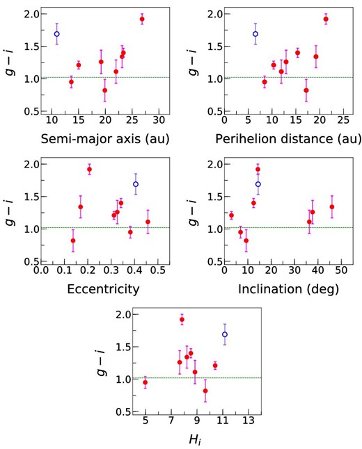
Dependence of g − i color on semi-major axis (a), perihelion distance (q), eccentricity (e), inclination (I), and measured absolute magnitude in the i band (Hi) for the nine Centaurs examined in the present work. The open circle represents 2014 AT28, which has a retrograde orbit and is not regarded as a Centaur in the definition by Gladman, Marsden, and Vanlaerhoven (2008)—see figure 1. The dashed line represents the solar color. (Color online)
The results of the above statistical analysis are shown in table 3. We found that the g − i color has a potentially significant correlation (i.e., the null hypothesis is rejected at a 0.05 level of significance) with semi-major axis. We found a similar result when we performed the test using a table for the case of small numbers (Ramsey 1989). Such a correlation was not found in the analysis of Terai et al. (2018) for TNOs observed by HSC-SSP. Although this positive correlation may reflect a certain evolutionary process of the Centaurs examined in the present work, further investigation is desirable to provide definite conclusions. On the other hand, table 3 shows that the correlation between color and perihelion distance is not significant for the objects we examined.
Previous works show that the onset of cometary activity in Centaurs and the disappearance of the very red material on their surfaces seem to begin at about q ∼ 10 au (Jewitt 2009, 2015). Jewitt (2009) argued that crystallization of amorphous ice, with the concomitant release of trapped volatiles, is the leading candidate process for the explanation of these observations. The absence of cometary activity in the 20 Centaurs discovered by Cabral et al. (2018) is consistent with this scenario. In fact, the top-right panel of figure 3 shows no object redder than the solar color for q ≲ 10 au, which seems consistent with the above argument. However, it is difficult to confirm the critical radial location of the change of the colors from our results since there is only one object (Chiron) on a prograde orbit with q < 10 au in our sample. Also, the color distribution of inactive Centaurs presented by Jewitt (2015) seems to be rather independent of q at q ≳ 10 au. Further investigation using a larger number of Centaurs, including those with smaller perihelion distance, is desirable.
In addition, we found no correlations of the g − i color with other orbital elements. By analyzing the colors of TNOs observed by the HSC-SSP, Terai et al. (2018) found that the color distribution as a function of orbital eccentricity can be divided into two groups, i.e., one group with low eccentricity and red color, and another group with relatively high eccentricity and neutral color (see their figure 11). They also found that the colors of those objects in the latter group have a positive correlation with eccentricity, while they showed a negative correlation with inclination. Such trends are not found for the eight Centaurs examined in the present work, which was also based on the HSC data. Recently, from an analysis of color data of 61 Centaurs, Tegler, Romanishin, and Consolmagno (2016) found that red Centaurs have significantly smaller orbital inclinations than gray Centaurs, while correlations between color and other orbital elements were not found (see also Tegler et al. 2008). Further studies are required to understand the implications of these observations for the origin and evolution of Centaurs.
As for the dependence of colors on absolute magnitude, Hainaut, Boehnhardt, and Protopapa (2012) showed that the color distribution of small bodies in the outer solar system seems to be size-independent, except that large ones are slightly bluer than the smaller ones in the near infrared (i.e., in the J − H color). On the other hand, Peixinho et al. (2012) found that the bimodal color distribution of Centaurs and TNOs is size-dependent (see also Peixinho et al. 2015). They found that not only Centaurs but also small TNOs with HR ≳ 6.8 (HR is the R-band absolute magnitude) have bimodal color distribution (see also Fraser & Brown 2012; Wong & Brown 2017), while such a bimodality is not seen for larger TNOs with 5 ≲ HR ≲ 6.8. Peixinho et al. (2012) noted that still larger TNOs with HR ≲ 5 show another bimodal color distribution. More recently, Tegler, Romanishin, and Consolmagno (2016) found that their entire sample of TNOs and Centaurs exhibited bimodal colors. They also found that the red Centaurs had average albedos about a factor of two larger than the gray Centaurs, while both populations had broadly similar absolute magnitude distribution, with a slight possibility of fainter absolute magnitude values for the red ones. This suggests that red Centaurs may have smaller diameters than gray Centaurs. The tendency that red objects have larger albedos has also been reported for Jupiter’s Trojans (Wong et al. 2014; see also Emery et al. 2011 and Grav et al. 2012). Although we did not find any correlation between the g − i color and absolute magnitude for the nine Centaurs we examined, the above studies suggest that examination of size dependence in a larger sample including bodies in other dynamical groups is important for a better understanding of the meaning of the color distribution of these bodies.
In order to understand how our data for the nine Centaurs fit in these previous studies with larger samples, we calculated spectral slopes from the g − i color for the nine objects in our sample and from the B − R color for the 61 Centaurs obtained by Tegler et al. (2008) and Tegler, Romanishin, and Consolmagno (2016), and compared them in figure 4 (see the Appendix for the calculations of these spectral slopes). Although we did not see bimodal color distribution for our nine objects alone (figure 2), in figure 4 seven objects of our sample seem to be in the gray group and the other two seem to belong to the red group in the bimodal distribution found by Tegler et al. (2008) and Tegler, Romanishin, and Consolmagno (2016). This strengthens the importance of using a large sample to find correlations that may yield useful constraints on the origin and evolution of these small bodies (Peixinho et al. 2015; Tegler et al. 2016).
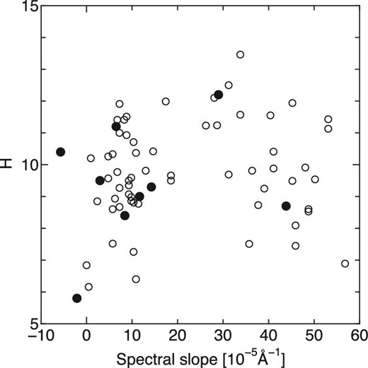
Relationship between absolute magnitude and spectral slope for Centaurs. The filled circles represent those calculated from the g − i color for the nine objects examined in the present work. The absolute magnitudes of these objects were obtained from the Minor Planet Center. Open circles represent those calculated from the B − R color for the 61 objects examined by Tegler et al. (2008) and Tegler, Romanishin, and Consolmagno (2016). The methods of calculation of the spectral slopes are described in the Appendix.
4 Conclusions and discussion
In the present work, we examined the color distribution of nine Centaurs observed by the Hyper Suprime-Cam (HSC) installed on the Subaru Telescope, and compared the results with the color distribution of TNOs also obtained by HSC (Terai et al. 2018). We found that the color distribution of the Centaurs we observed is not significantly different from that of the TNOs with high orbital inclinations (>6°), while it is distinct from that of cold classical TNOs with low orbital inclinations (<6°). This result suggests that TNOs with high orbital inclinations and Centaurs have a common origin. This view is also consistent with recent works using larger samples that show that the bimodal color distribution is seen not only for Centaurs but also for both small and large TNOs (Peixinho et al. 2012; Fraser & Brown 2012; Tegler et al. 2016; Wong & Brown 2017). Although we did not see the bimodal color distribution found in previous studies (Peixinho et al. 2003; Tegler et al. 2003) in our sample alone, by comparing spectral slopes obtained from our data with those calculated from B − R colors of larger samples obtained by previous works (Tegler et al. 2008, 2016), we found that seven and two Centaurs in our sample belong to the gray and red groups, respectively.
We also investigated correlations of the color distribution of these Centaurs with other quantities, i.e., orbital elements and absolute magnitude. While we found a potentially significant positive correlation between the color and semi-major axis, no significant correlations were found with other orbital elements. On the other hand, recent works with larger samples show that red Centaurs have significantly smaller orbital inclinations than gray Centaurs, while no significant correlations were found between the color and other orbital elements (Tegler et al. 2016). We did not find correlation between the color and absolute magnitude for the nine objects we examined, but recent works with larger samples show that the bimodal color distribution is size-dependent (Peixinho et al. 2012, 2015; Fraser & Brown 2012; Tegler et al. 2016; Wong & Brown 2017). Further investigation with a larger number of samples is desirable to confirm these findings.
The observed color distribution of Centaurs may be linked to space weathering, collisional evolution, cometary activity (Hainaut & Delsanti 2002; Jewitt 2009, 2015), or a combination of these and other processes (e.g., intrinsic composition for distinct formation birthplaces). Also, Centaurs can possess ring systems (Braga-Ribas et al. 2014; Ruprecht et al. 2015; Ortiz et al. 2015). Models for the formation of such ring systems include collisional ejection from the parent body’s surface, disruption of a primordial satellite, dusty outgassing (Pan & Wu 2016), and partial disruption of the parent body during a planetary encounter (Hyodo et al. 2016). The possession of ring systems (Ortiz et al. 2015) as well as their formation process may also be linked to the Centaur color bimodality. Further observations of Centaurs, TNOs, and other small solar system bodies are essential to better understand the origin and evolution of Centaurs and their parent population.
Funding
This work was supported by JSPS KAKENHI Nos. 18K13607 (T.T.), 15H03716, 16H04041 (K.O.), and 16K05546 (F.Y.).
Acknowledgments
We thank the anonymous reviewer for detailed comments and suggestions, which greatly improved the presentation of the manuscript. We also thank Fumihiko Usui for discussion and comments on our work, and Chien-Hsiu Lee for comments on the manuscript.
This study is based on data collected at the Subaru Telescope and retrieved from the HSC data archive system, which are operated by the Subaru Telescope and Astronomy Data Center, National Astronomical Observatory of Japan. The Hyper Suprime-Cam (HSC) collaboration includes the astronomical communities of Japan and Taiwan, and Princeton University. The HSC instrumentation and software were developed by the National Astronomical Observatory of Japan (NAOJ), the Kavli Institute for the Physics and Mathematics of the Universe (Kavli IPMU), the University of Tokyo, the High Energy Accelerator Research Organization (KEK), the Academia Sinica Institute for Astronomy and Astrophysics in Taiwan (ASIAA), and Princeton University. Funding was contributed by the FIRST program from the Japanese Cabinet Office, the Ministry of Education, Culture, Sports, Science and Technology (MEXT), the Japan Society for the Promotion of Science (JSPS), the Japan Science and Technology Agency (JST), the Toray Science Foundation, NAOJ, Kavli IPMU, KEK, ASIAA, and Princeton University. This paper makes use of software developed for the Large Synoptic Survey Telescope. We thank the LSST Project for making their code available as free software at 〈http://dm.lsst.org〉. The Pan-STARRS1 Surveys (PS1) have been made possible through contributions of the Institute for Astronomy, the University of Hawaii, the Pan-STARRS Project Office, the Max-Planck Society and its participating institutes, the Max Planck Institute for Astronomy, Heidelberg and the Max Planck Institute for Extraterrestrial Physics, Garching, the Johns Hopkins University, Durham University, the University of Edinburgh, Queen’s University Belfast, the Harvard-Smithsonian Center for Astrophysics, the Las Cumbres Observatory Global Telescope Network Incorporated, the National Central University of Taiwan, the Space Telescope Science Institute, the National Aeronautics and Space Administration under Grant No. NNX08AR22G issued through the Planetary Science Division of the NASA Science Mission Directorate, the National Science Foundation under Grant No. AST-1238877, the University of Maryland, Eotvos Lorand University (ELTE), and the Los Alamos National Laboratory.
Appendix. Calculation of spectral slopes from B − R and g − i colors
References
