


Abstract
Faraday tomography is thought to be a powerful tool to explore the cosmic magnetic field. Broadband radio polarimetric data are essential to ensuring the quality of Faraday tomography, but such data are not easy to obtain because of radio frequency interferences. In this paper, we investigate optimum frequency coverage of Faraday tomography so as to explore the Faraday rotation measure (RM) due to the intergalactic magnetic field (IGMF) in filaments of galaxies. We adopt a simple model of the IGMF and estimate confidence intervals of the model parameters using the Fisher information matrix. We find that meaningful constraints on RM due to the IGMF are available with data at multiple narrowbands which are scattered over the ultra-high frequency (UHF, 300–3000 MHz). The optimum frequency depends on the Faraday thickness of the Milky Way foreground. These results are obtained for a wide brightness range of the background source including fast radio bursts. We discuss the relation between the polarized-intensity spectrum and the optimum frequency.
1 Introduction
The magnetic field is a fundamental element of the Universe and it affects the formation and evolution of astronomical objects. Centimeter radio polarimetry is one of the promising tools for the study of cosmic magnetism (see Han 2017; Akahori et al. 2018 for reviews): synchrotron intensity, its linear-polarization vector, and the Faraday rotation measure (RM) provide us with the properties of the magnetic field in galaxies and active galactic nucleus (AGN) jets, and they reveal detailed structures of magnetized plasma such as the interstellar medium (ISM) and intergalactic medium (IGM). Cosmic magnetism is one of the key sciences for the Square Kilometre Array (SKA) (Johnston-Hollitt et al. 2015).
Faraday RM synthesis or Faraday tomography (Burn 1966; Brentjens & de Bruyn 2005) makes progress in radio polarimetry. There are a lot of successful applications to the ISM (Sakemi et al. 2018), galaxies (Mao et al. 2017), radio lobes (O’Sullivan et al. 2018), quasars (Anderson et al. 2015, 2016), and galaxy clusters (Ozawa et al. 2015). Furthermore, the discovery of fast radio bursts (FRBs) fosters momentum of the study of cosmic magnetism. Since 2018 April, details of seven linearly-polarized FRBs have been available in the literature (see Caleb et al. 2018). For example, Michilli et al. (2018) observed FRB 121102 and found a strongly magnetized medium with RM ∼ O(105) rad m−2, implying an environment similar to that around a super-massive black hole (SMBH).
It has been predicted that the cosmic web is permeated with a large amount of magnetized IGM. Akahori et al. (2014a) studied possible situations to estimate RM due to the intergalactic magnetic field (IGMF) by means of Faraday tomography, and demonstrated that the ultra-high frequency (UHF) band is promising for maximizing the capability of Faraday tomography for the study. Ravi et al. (2016) applied Faraday tomography to FRB 150807 and derived an upper limit of the IGMF strength <21 nG, which does not contradict theoretical predictions (e.g., Akahori et al. 2016; Vazza et al. 2018).
The above studies demonstrate the capability of Faraday tomography for a wide RM range of diffuse, compact, and even time-domain radio sources. Because wider frequency coverage gives a better quality of Faraday tomography (e.g., Akahori et al. 2014a), a modern wideband observation makes Faraday tomography feasible. However, obtaining a seamless data set over a broad bandwidth is difficult. One of the essential reasons is radio frequency interferences (RFIs). Centimeter wavelength is commonly used in many industries, such as broadcasting, mobile phone, wireless communications, and radar industries. Figure 1 shows an example of RFIs (see the Appendix for observational details). The appreciable signals are all RFIs against radio astronomy. These RFIs easily saturate amplifiers, produce artificial higher-harmonic signals, and alter the band characteristics fatally; therefore, they make signal processing unreliable.
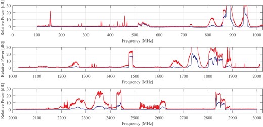
Radio frequency environment around the Kashima 34 m antenna of the National Institute of Information and Communications Technology (NICT) in Japan. The blue and red lines show the instantaneous (sweep time 2.05 s) and 5 min max-hold (i.e., maximum for 5 min) spectra, respectively. The band characteristic of the receiver is removed from the spectra, so that the vertical axis is the relative radio power with respect to the detection limit. (Color online)
Persistent RFIs can be cut by frequency filters at an early stage of a receiver system, but this means that we never obtain astronomical signals at those frequencies. Although many large radio telescopes are located in the countryside, where the population is low, the radio frequency environment rapidly changes as the lifestyle improves.1 SKA-MID antennas will be constructed in radio-quiet districts in South Africa, but economic growth in South Africa could impact on the radio frequency environment at the site in future.
In this paper, we investigate the optimum frequency of Faraday tomography to explore RM due to the IGMF. Although Akahori et al. (2014a) briefly considered RFIs on the SKA sites, a more comprehensive study of frequency dependence on Faraday tomography could maximize the chance to discover the IGM and IGMF through Faraday tomography. This paper is organized as follows. We explain our model and calculation in section 2. The results are shown in section 3, followed by discussion and summary in section 4.
2 Model and calculation
Our model and calculation are mostly the same as the previous works (Akahori et al. 2014a; Ideguchi et al. 2014a). Akahori et al. (2014a) studied two cases of observations, (i) background compact source behind diffuse foreground source, and (ii) two pair compact sources. This paper addresses case (i). Below, we briefly review our model and calculation, more details can be found in the above references.
2.1 Model
The top panel of figure 2 shows an example of an FDF model. We assume that we select spatially compact sources such as quasars, radio galaxies, or FRBs and choose an ideal Faraday-thin source whose thickness in the Faraday-depth space is sufficiently small compared to the resolution of the Faraday depth (see, e.g., Akahori et al. 2018). We also suppose that there is no intervening galaxy along the LOS toward the source. This source then appears at a certain Faraday depth induced by RMs mostly due to the IGMF and the Milky Way. The Milky Way can be bright and likely appear as a Faraday-thick source, so that the gap between the two signals in ϕ space becomes a measure of RM due to the IGMF (Akahori et al. 2014a; see also Akahori et al. 2014b for a source selection strategy).
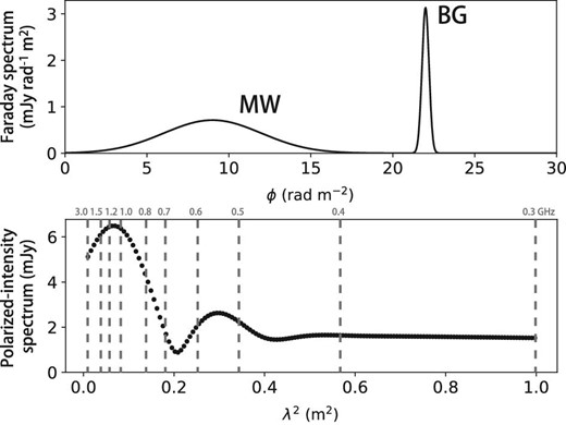
Examples of a Faraday spectrum (top) and a polarized-intensity spectrum (bottom).
2.2 Calculation
We adopt a model-fitting method in which we compare the observed data with a numerical model and find the best model parameters that minimize the chi-squared value. In reality, the transformation from the observed Stokes Q and U to the FDF is always imperfect due to the incompleteness of the wavelength coverage, while the transformation from a model FDF to Stokes Q and U can reduce this numerical error thanks to the reduced incompleteness of the Faraday-depth coverage. Therefore, we compare the observed (mock) polarized-intensity spectrum with the spectrum given by our model FDF. This approach is called “QU-fitting.”
The bottom panel of figure 2 shows an example of the polarized-intensity spectrum derived from a Fourier transform of the example FDF (figure 2, top). To this synthesized spectrum, we add two observational effects—frequency coverage and noise—and construct a mock polarization spectrum data, as follows.
Frequency coverage is the main concern of this work. According to previous work (Akahori et al. 2014a), we consider the UHF (300–3000 MHz) band which is promising for the study of the IGMF. Particularly, we examine the optimum frequency at low frequency (300–1000 MHz) in the UHF, because the dependence of the polarized-intensity spectrum on λ2 is significant in this band (see figure 2 bottom). Meanwhile, at high frequency (1000–3000 MHz), the dependence is minor and the fine-tuning of band selection does not significantly change the result. Therefore, we employ fixed, given narrowbands which are motivated by radio quietness at high frequency in the UHF (e.g., figure 1).2 Table 1 summarizes the band definitions used in this work. We consider one broadband (L) and/or three narrowbands labeled L14, L16, and S27. Here and throughout this work, one frequency channel or the frequency resolution is 1 MHz, following modern large polarization surveys (e.g., the polarization sky survey of the Universe’s magnetism, POSSUM). We then explore the best center frequency of the P* band with a narrow bandwidth of 20 MHz or 40 MHz (20 channels or 40 channels). The above frequency coverage is applied to the Faraday spectrum by convolution using the window function approach (Akahori et al. 2014a).
Frequency band definition in this work.
| Band | Minimum | Center | Maximum | Bandwidth |
|---|---|---|---|---|
| (MHz) | (MHz) | (MHz) | (MHz) | |
| P * | 300 | — | 1000 | 20 or 40 |
| L | 1000 | 1500 | 2000 | 1000 |
| L 14 | 1400 | 1410 | 1420 | 20 |
| L 16 | 1500 | 1550 | 1600 | 100 |
| S 27 | 2650 | 2700 | 2750 | 100 |
| Band | Minimum | Center | Maximum | Bandwidth |
|---|---|---|---|---|
| (MHz) | (MHz) | (MHz) | (MHz) | |
| P * | 300 | — | 1000 | 20 or 40 |
| L | 1000 | 1500 | 2000 | 1000 |
| L 14 | 1400 | 1410 | 1420 | 20 |
| L 16 | 1500 | 1550 | 1600 | 100 |
| S 27 | 2650 | 2700 | 2750 | 100 |
Observational noise, or the sensitivity, is considered as follows. We consider flat-frequency spectra of both MW and BG sources, meaning that the intrinsic polarized-intensity of the sources does not change in frequency. We add a random Gaussian noise, where the signal-to-noise ratio in each 1 MHz channel is 10 for MW and 100, 1000, or 10000 for BG. Hence, if we suppose a 100 μJy noise level, we are considering a Milky Way foreground of 1 mJy and a background source range of from 10 mJy to 1 Jy.
3 Result
3.1 Optimum frequency of the P* band
We first consider full coverage of the L band. This makes the situation simple and allows us to examine the importance of the P* band. Figure 3 shows the results. The horizontal axis is the input RMIGMF and the vertical axis is the center frequency of the P* band. The blue, green, and red lines show the contours on which RMIGMF's are determined with statistical errors of 30%, 20%, and 10%, respectively, based on the confidence intervals given by the Fisher information matrix.
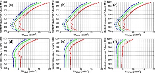
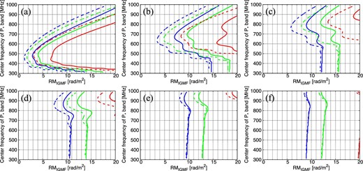
Error profiles between the input RMIGMF and the chosen center frequency of the P* band. Results in the cases of the P* + L bands are shown. The blue, green, and red lines show the contours on which RMIGMF's are determined with statistical errors of 30%, 20%, and 10%, respectively. The solid and dashed lines are the results with 20 MHz and 40 MHz bandwidths of the P* band, respectively. Panels (a), (b), and (c) are the results for FBG/FMW = 10, 100, and 1000, respectively, with δϕMW = 2 rad m−2. Panels (d), (e), and (f) are the results for δϕMW = 4, 6, and 8 rad m−2, respectively, with FBG/FMW = 100. (Color online)
The solid lines indicate the results with a 20 MHz bandwidth of the P* band. For example, in figure 3a, we safely obtain RMIGMF = 10 rad m−2 with a statistical error less than 10%, if we choose the center frequency of the P* band to be from 300 MHz to 750 MHz. We achieve a 10% error-level detection of RMIGMF ∼ 5 rad m−2 (i.e., we can measure RMIGMF = 5 ± 0.5 rad m−2), if we choose the center frequency of the P* band to be around 500 MHz.
The situation can be improved if a 40 MHz bandwidth of the P* band is available (dashed lines): in figure 3a, an error level of 10% for RMIGMF = 5 rad m−2 ranges from 370 MHz to 580 MHz. Even if we accept the error level of 30%, we can obtain RMIGMF down to ∼1 rad m−2 with a 40-MHz bandwidth at 450 MHz.
Figures 3a–3c compare the effects of intensity ratios, fBG/fMW. Surprisingly, we see that the intensity ratio does not significantly alter the results at least within the shown range, fBG/fMW = 10–1000. Such independence in the intensity ratio can be seen in most of the results shown in this paper. Therefore, hereafter we only show the results for the case of the intensity ratio fBG/fMW = 100.
Figures 3d–3f show the results for δϕMW = 4, 6, and 8 rad m−2, respectively. Comparing those with figure 3b, the optimum frequency shifts to higher frequency. It indicates that the optimum frequency depends on the thickness of the Milky Way foreground emission. We also see that an increase of the bandwidth of the P* band does not significantly improve the result, if δϕMW is relatively large.
3.2 Impact of the narrow L band
Figure 4 shows the optimum frequency of the P* band in the cases with the two narrow L bands (L14 + L16). Overall, the lack of data in the L band makes the constraint of RMIGMF worse, but we still obtain RMIGMF with a reasonable error. For example, in figure 4a, we obtain RMIGMF = 10 rad m−2 with a statistical error less than 10%, if we choose the center frequency of the P* band from the range 380–610 MHz with a 20 MHz bandwidth. With a 40 MHz bandwidth, it improves to RMIGMF = 5 rad m−2 for the center frequency of the P* band in the range 400–550 MHz.
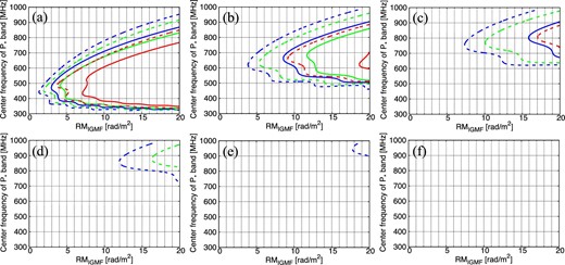
Same as figure 3 but in the cases of the P* + L14 + L16 bands for δϕMW = 2, 4, 6, 8, 10, 12 rad m−2 from (a) to (f), respectively, with FBG/FMW = 100. (Color online)
Note that, compared to figure 3, we may need a more careful choice of the center frequency of the P* band: error levels quickly get worse as the center frequency deviates from the optimum frequency. For example, in figure 4a, when we set the center frequencies at ∼500 MHz, ∼650 MHz, and ∼800 MHz with a 40 MHz bandwidth, we achieve 10% error-level detections of RMIGMF = 4, 9, and 17 rad m−2, respectively.
We again see the dependence on δϕMW. The optimum frequencies of the P* band for δϕMW = 2, 4, and 6 rad m−2 are ∼500 MHz, ∼650 MHz, and ∼800 MHz, respectively. These optimum frequencies are similar to those in figure 3. Contrary to the result seen in figures 3d–3f, increasing the bandwidth of the P* band substantially improves the results even in large δϕMW cases. If δϕMW exceeds ∼10 rad m−2, however, we cannot constrain RMIGMF within the error range from the data of the three narrowbands.
3.3 Improvement by the narrow S band
From the results in previous sections, we expect that high-frequency (S band) data is useful when the MW foreground is thicker (in cases of low and mid galactic latitudes). Therefore, for the calculation in the previous section, we add the data of the S27 narrowband and the results are shown in figure 5.
Same as figure 3 but in the cases of the P* + L14 + L16 + S27 bands for δϕMW = 2, 4, 6, 8, 10, 12 rad m−2 from (a) to (f), respectively, with FBG/FMW = 100. (Color online)
We see that the data at the S27 band moderately improve the result in the cases of δϕMW = 2 and 4 rad m−2. On the other hand, as expected, improvement is significant in the thicker cases. Increasing the bandwidth of the P* band improves the results for thicker MW foreground. If we allow the error level of 30%, we obtain RMIGMF down to ∼8 rad m−2 with a 40 MHz bandwidth at 800–900 MHz, in the cases with δϕMW ∼ 8–10 rad m−2.
4 Discussion and summary
where we consider a flat spectral index (in the case of α = 0 of Arshakian & Beck 2011) and |$k=2 |RM| \lambda _{\rm opt}^2$|. The optimum frequencies that we found are in broad agreement with the solution of k = 2.0288 (radian) for an effective RM value of |RM| ∼ 1.3δϕMW. Therefore, the optimum frequencies can be explained by the depolarization theory.
The above depolarization frequency, i.e., the optimum frequency, depends on the model Faraday spectrum of the Milky Way: we have considered a Gaussian shape and the intrinsic polarization angle is constant. We can consider more complicated, realistic FDFs of polarized sources (Ideguchi et al. 2014b). However, this work focuses on a typical, global solution of the optimum frequency. A specific model is beyond the scope of this work and it will be considered in a separate paper. Nevertheless, if an actual Faraday spectrum of the Milky Way deviates from the Gaussian, the depolarization frequency can change. Note that the constraint on RMIGMF, i.e., the gap between MW and BG, primarily depends on the edge of the Faraday spectrum of the Milky Way rather than a detailed profile of the Faraday spectrum of the Milky Way.
Throughout this paper, the total intensity is independent from the frequency so that a flat spectral index is considered. If we consider a steep spectrum, the intensity of the P* band becomes brighter and the signal-to-noise ratio becomes better by several times. This may result in better constraints on RMIGMF, because we obtain a better quality of data at the P* band. We will address this effect more quantitatively in future, since Faraday tomography considering a non-zero spectral index is under development.
The intensity ratio between the background and foreground sources does not significantly change the results, and exceptionally bright (Jy-level) background sources are available to this work of exploring the IGMF. Therefore, our method can be applicable for background, linearly-polarized FRBs. Meanwhile, detection of the Milky Way foreground would be more challenging. We have considered the signal-to-noise ratio of 10 for MW in each 1 MHz channel. If the noise level is higher, it seriously impacts the detection of the Milky Way. Moreover, an interferometric observation may suffer from the missing flux of diffuse foreground emission.
Although we introduced RFIs in Kashima as an example, our results do not depend on where and how the polarized intensity spectrum is obtained. Therefore, our results can be applicable to other current radio facilities and even the future telescopes such as the SKA.
A possible recipe to confront this Milky Way foreground issue would be that we combine this work with another single-dish observation of the diffuse Milky Way foreground. A comparison between on-source and off-source observations is also useful, where the off-source observation measures a nearby sky sharing almost the same foreground. These follow-up observations confirm the diffuse foreground and decide the edge of the Faraday spectrum of the Milky Way. If we have two background sources located closely to each other, we can apply another methodology, case (ii), discussed in Akahori et al. (2014a).
In summary, we studied optimum frequencies to constrain the Faraday rotation measure (RM) due to the IGMF by means of Faraday tomography. The frequency resolution of 1 MHz has been considered throughout this work. Using a simple model and the Fisher information matrix, we find that multiple narrowband data in the UHF provide a reasonable constraint on the RM due to the IGMF. With data at 1400 MHz and 1600 MHz, RMIGMF ∼ 10 rad m−2 toward a high Galactic latitude is detectable with less than 10% error, if we choose the center frequency of the P* band around 400–700 MHz with a 40 MHz bandwidth.
Acknowledgments
This work was supported in part by JSPS KAKENHI Grant Numbers JP15H05896 (KT), JP16H05999 (KT), JP16K13788 (T. Aoki), JP17K01110 (T. Akahori, KT), and Bilateral Joint Research Projects of JSPS (KT). Numerical computations were carried out on PC cluster at Center for Computational Astrophysics, National Astronomical Observatory of Japan.
Appendix. RFI observation at Kashima
We investigated the radio environment at NICT Kashima in daytime and nighttime on 2017 August 28, JST. It was cloudy and slightly windy. We measured radio spectra between 100 MHz and 1000 MHz using a discone antenna and radio ones between 1000 MHz to 3000 MHz with a tear-drop antenna. Antennas were placed on a pedestal of the rooftop of the operation center so as to ensure that a height of the antenna exceeds that of the metal fence enclosing the rooftop. Band characteristics were measured by replacing an antenna with a terminator and were removed from the RFI data. The data were visualized with a spectrum analyzer. Modes of the spectrum analyzer were instantaneous (blue) and 5 min max-hold (orange), where we set the resolution bandwidth (RBW) at 1 MHz and the video bandwidth (VBW) at 1 kHz. The results obtained around 11 p.m. are shown in figure 1. We observed that the shown spectrum is time-dependent.
The beam patterns of the both antennas are torus-like and hence the antennas have the highest sensitivity to the ground, horizontal direction. They only have a capability to capture vertical polarization with respect to the ground plane. Therefore, the results do not fully cover RFIs coming from the top of the antenna or RFIs of horizontal polarization coming from all horizontal directions. For instance, most of television broadcasts in Japan are of horizontal polarization, which is not sensitive in our experience. Therefore, its effect is likely underestimated. Since the antenna is omnidirectional, it is difficult to identify the locations of the origins of the RFIs.
Footnotes
Indeed, “Sky Muster” RFIs at the ATCA 15 mm band and “BSAT-4a” RFIs at the VERA K band have appeared very recently.
Part of the radio-quiet bands are recognized for usage of radio astronomy as primary (passive) or secondary.
References
