


Abstract
We present an X-ray study of the mixed-morphology supernova remnant CTB 1 (G116.9+0.2) observed with Suzaku. The 0.6–2.0 keV spectra in the northeastern breakout region of CTB 1 are well represented by a collisional ionization-equilibrium plasma model with an electron temperature of ∼0.3 keV, whereas those in the southwestern inner-shell region can be reproduced by a recombining plasma model with an electron temperature of ∼0.2 keV, an initial ionization temperature of ∼3 keV, and an ionization parameter of ∼9 × 1011 cm−3 s. This is the first detection of the recombining plasma in CTB 1. The electron temperature in the inner-shell region decreases outwards, which implies that the recombining plasma is likely formed by the thermal conduction via interaction with the surrounding cold interstellar medium. The Ne abundance is almost uniform in the observed regions whereas Fe is more abundant toward the southwest of the remnant, suggesting an asymmetric ejecta distribution. We also detect a hard tail above the 2-keV band that is fitted with a power-law function with a photon index of 2–3. The flux of the hard tail in the 2–10 keV band is ∼5 × 10⁻¹³ erg cm−2 s−1 and peaks at the center of CTB 1. Its origin is unclear but one possibility is a putative pulsar wind nebula associated with CTB 1.
1 Introduction
Mixed-morphology supernova remnants (MM SNRs) have a characteristic morphology of a radio shell with centrally-filled thermal X-rays (Rho & Petre 1998). Most of the MM SNRs are likely interacting with a dense interstellar medium (ISM) as indicated by detections of CO emissions or OH masers at 1720 MHz in some cases (e.g., Tatematsu et al. 1990; Rho & Petre 1998; Yusef-Zadeh et al. 2003). Some of them are also associated with GeV gamma-ray emissions (e.g., Acero et al. 2016), supporting the presence of a dense ISM in the vicinity of the remnants if the origin of the gamma-ray is π0 decays. Such a dense surrounding environment probably plays an important role in the formation of MM SNRs, but detailed physical processes are still under debate (e.g., White & Long 1991; Cox et al. 1999).
Recently, X-ray observations found recombining plasmas (RPs) in many MM SNRs (e.g., Kawasaki et al. 2002; Yamaguchi et al. 2009; Ozawa et al. 2009; Ohnishi et al. 2011; Sawada & Koyama 2012; Uchida et al. 2012; Matsumura et al. 2017b). An RP indicates the unusual evolution of thermal plasmas, because the ionization timescale is longer (≳ 105 yr) than the typical age of SNRs in the typical density of electrons (0.1–1 cm−3) and an ionizing plasma is expected in SNRs. For the formation of RPs in MM SNRs, two scenarios are mainly considered. One of the proposed scenarios is a rapid decreasing of the electron temperature (kTe) via the rarefaction of the plasma when the shock breaks out of the dense circumstellar medium into low density ISM (Itoh & Masai 1989). The other is the thermal conduction scenario, in which kTe decreases rapidly due to the interaction between the surrounding cold ISM and the hot plasmas (Kawasaki et al. 2002; Matsumura et al. 2017b).
CTB 1 (G116.9+0.2) is one of the MM SNRs. It has a characteristic morphology as shown in figure 1; its non-thermal radio shell breaks at the northeastern quadrant (Landecker et al. 1982; Kothes et al. 2006) and its thermal X-rays extend outward from the break region (Craig et al. 1997). Optical emission lines also show an incomplete shell morphology similar to the radio shell (Fesen et al. 1997). Yar-Uyaniker, Uyaniker, and Kothes (2004) argued that CTB 1 is located inside a large H i bubble, and that the radio shell is interacting with the edge of the bubble. No detections of gamma-ray emissions have been reported so far (e.g., Acero et al. 2016). The distance to the remnant is highly uncertain in the range of 1.6–3.1 kpc (Craig et al. 1997; Yar-Uyaniker et al. 2004). The SNR age is estimated to be a few 104 yr (Koo & Heiles 1991; Hailey & Craig 1994).
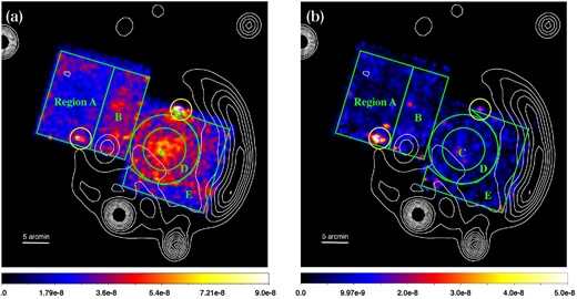
Exposure-corrected XIS images of CTB 1 in the (a) 0.6–2.0 keV band and (b) 2.0–5.0 keV band. The contours are a radio intensity map observed with the Canadian Galactic Plane Survey at 408 MHz (Kothes et al. 2006). The magenta crosses with the yellow circles indicate bright point sources excluded in the spectral analyses. The green regions labeled with A, B, C, D, and E are spectral extraction regions (see sub-subsection 3.2.4). (Color online)
The nature of the thermal X-rays of CTB 1 has been studied via ASCA and Chandra observations by Lazendic and Slane (2006) and Pannuti et al. (2010). Their results show that a primary component is a thermal plasma in collisional ionization equilibrium (CIE) with kTe ∼ 0.2–0.3 keV. However, they reported different minor components probably due to different analysis methods. Lazendic and Slane (2006) argued that another high-temperature plasma (kTe ∼ 0.8 keV) is present inside the radio shell, whereas Pannuti et al. (2010) claimed a detection of a significant hard tail represented by a very high-temperature plasma (kTe ∼ 3 keV) or a power-law function with a photon index (Γ ∼ 2–3) in both the inner radio shell and the breakout regions. Therefore, the nature of the X-ray plasmas is still unclear.
Here, we present new X-ray observations of CTB 1 with Suzaku (Mitsuda et al. 2007). Due to low instrumental background, the X-ray CCDs aboard Suzaku have very high sensitivity to diffuse sources in the 0.6–5.0 keV band and are suitable to reveal a precise physical property of CTB 1. Throughout this paper, statistical errors are quoted at a 68% (1 σ) confidence level.
2 Observation and data reduction
We observed the southwestern (SW) and northeastern (NE) regions of CTB 1 with the X-ray Imaging Spectrometer (XIS: Koyama et al. 2007) aboard the Suzaku satellite. The XIS has three front-illuminated (FI) CCDs (XIS 0, 2, 3) and one back-illuminated (BI) CCD (XIS 1). The observation log is shown in table 1. The total effective exposure time is ∼82 ks.
Observation log.
| Target name | Ods. ID | Obs. date | l | b | Effective exposure |
|---|---|---|---|---|---|
| CTB 1_SW | 506034010 | 2011-12-29 | |${116^{\circ}8913}$| | |${0^{\circ}2952}$| | 29 ks |
| CTB 1_NE | 506035010 | 2011-12-28 | |${117^{\circ}1835}$| | |${0^{\circ}1796}$| | 53 ks |
| GALACTIC PLANE 111 (BG1) | 501100010 | 2006-06-06 | |${111^{\circ}5011}$| | |${1^{\circ}3149}$| | 72 ks |
| ANTICENTER2 (BG2) | 503006010 | 2008-08-01 | |${122^{\circ}9896}$| | |${0^{\circ}0395}$| | 86 ks |
In order to evaluate a background spectrum, we also used nearby archival observations of GALACTIC PLANE 111 and ANTICENTER2 (hereafter BG1 and BG2, respectively). As shown in table 1, the pointing direction of BG1 and BG2 are ∼5° away from CTB 1 in the Galactic latitude, but are on the Galactic plane. Therefore, an average spectrum of BG1 and BG2 likely represents a background spectrum at the coordinates of CTB 1. We also confirmed that no bright sources are included in the XIS fields-of-view (FoVs) of BG1 and BG2.
We processed the above XIS data with the HEADAS software version 6.20 and the calibration database released in 2016 December. We started with cleaned event lists produced by the standard pipeline process. The data taken by the 3 × 3 and 5 × 5 editing modes were merged. We discarded cumulative flickering pixels and pixels adjacent to the flickering pixels according to the noisy pixel maps provided by the XIS team.1 Events below 0.6 keV were not used because contamination of O i Kα from the sunlit-Earth atmosphere in our observations was more severe than that shown in Sekiya et al. (2014), and spectral modeling below 0.6 keV is highly uncertain even when we add a Gaussian for O i Kα. The XIS 2 and part of the XIS 0 have not been functional since anomalies occurred in 2006 November and in 2009 June, respectively. We therefore do not use the entire XIS 2 or segment A of XIS 0.
3 Analysis
3.1 XIS Images of CTB 1
Figure 1 shows exposure-corrected XIS images of CTB 1 in the 0.6–2.0 keV band and the 2.0–5.0 keV band. The data of XIS 0, 1, and 3 were co-added, and the non X-ray backgrounds (NXBs) estimated by xisnxbgen (Tawa et al. 2008) were subtracted. As already reported by Lazendic and Slane (2006) and Pannuti et al. (2010), soft X-ray emission in the 0.6–2.0 keV band is concentrated at the center of the radio shell and extends toward the break of the radio shell. On the other hand, no remarkable diffuse structures are seen in the 2.0–5.0 keV band image.
We found two bright point sources at the southern edge of the NE observation and the northern edge of the SW observation. They were also identified in the 2XMMi catalog (Watson et al. 2009) and have fluxes of ∼4 × 10⁻¹³ erg cm−2 s−1. In the following spectral analyses, we excluded those point sources by the circular regions with 2΄ radii as shown in figure 1.
3.2 Spectral modeling
In this section, we performed spectral modeling using the XSPEC version 12.9.1a. We extracted 0.6–10.0 keV and 0.6–8.0 keV spectra from the FI CCDs and BI CCD, respectively, and then subtracted corresponding NXB spectra created by xisnxbgen from them. Redistribution matrix files and auxiliary response files were generated by xisrmfgen and xissimarfgen (Ishisaki et al. 2007), respectively. The FI and BI CCDs spectra were simultaneously fitted.
3.2.1 Background estimation
Before analyzing the spectra of CTB 1, we estimated background spectra using the BG1 and BG2 observations. Figure 2 shows spectra extracted from the entire FoVs of those background observations. Continua dominate the spectra and weak emission lines were seen below 2 keV.
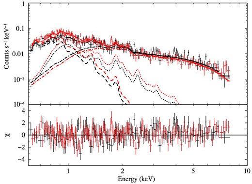
XIS 1 spectra of BG1 (black) and BG2 (red) after the NXB subtraction. The solid curves show the Galactic background model described in section 3.2.1. The dashed, dotted, and dash–dotted curves indicate the APEC1, the APEC2, and the CXB components, respectively. (Color online)
The best-fitting model and parameters are shown in figure 2 and table 2, respectively. The model represents the spectra with |$\chi ^2_\nu = 1.21$|. The obtained plasma temperatures of 0.21 and 0.96 keV agree with the typical temperature range of coronal X-rays (Johnstone & Güdel 2015). We found that the surface brightness of the stellar component is different by a factor of 2 between BG1 and BG2. Since CTB 1 is located in the middle of BG1 and BG2, CONST was fixed at the average of them (1.5) in the following spectral analyses of CTB 1. We confirmed that our results were not affected even when CONST was fixed to 1 or 2.
Best-fitting parameters of the background.*
| Model | Parameter (unit) | Value |
|---|---|---|
| CONST | Factor of BG1 | 1.0 (fixed) |
| Factor of BG2 | 2.0 ± 0.1 | |
| PHABS1 | N H (1021 cm−2) | 5.8 ± 0.5 |
| APEC1 | kT e (keV) | |$0.21^{+0.01}_{-0.02}$| |
| Z (solar) | 1.0 (fixed) | |
| N † (1011 cm−5) | |$1.6^{+0.9}_{-0.4}$| | |
| APEC2 | kT e (keV) | |$0.96^{+0.05}_{-0.04}$| |
| Z (solar) | 1.0 (fixed) | |
| N † (1011 cm−5) | 0.16 ± 0.02 | |
| PHABS2 | N H of BG1 (1021 cm−2) | 7.63 (fixed) |
| N H of BG2 (1021 cm−2) | 7.38 (fixed) | |
| PL | Γ | 1.4 (fixed) |
| Surface brightness‡ | 5.3 (fixed) | |
| χ2/d.o.f. | 875.52/726 |
*Parameters are common between BG1 and BG2 except for CONST and PHABS2.
†Normalization of the APEC component is |$\frac{1}{4\pi D^2} \int n_{\rm e}n_\mathrm{H}dV$|, where D is the distance to the source, ne and nH are the electron and hydrogen densities, respectively, and V is the X-ray emitting volume.
‡Units of 10−15 erg cm−2 s−1 arcmin−2 in the 2.0–10.0 keV band.
3.2.2 Spectra of the NE region
Spectra extracted from the entire FoV of the NE observation of CTB 1 are shown in figure 3a. Strong emission lines of highly ionized O, Ne, and Mg are present below 2 keV while no remarkable features are seen above 2 keV.
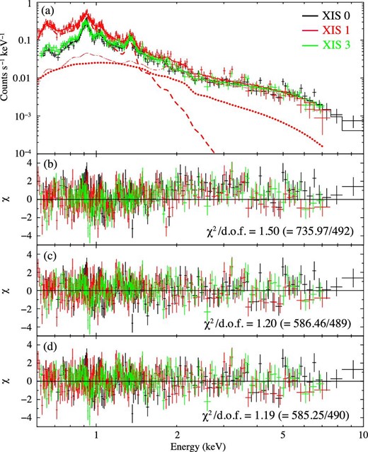
Top panel (a) shows spectra of the NE observation taken by the XIS 0 (black), 1 (red), and 3 (green). The solid curves are NE Model3. The dashed, dotted, and dash–dotted curves represent the VAPEC, the PL, and the background components of XIS 1, respectively. The lower three panels show the residuals of the data compared to NE Model1 (b), NE Model2 (c), and NE Model3 (d). (Color online)
According to Pannuti et al. (2010), we modeled those spectra using a single CIE plasma model with variable abundances of individual metals (the VAPEC model). Abundances of Ne, Mg, Si, and Fe were allowed to vary. Abundances of S and Ni were linked to those of Si and Fe, respectively. If the O abundance was treated as a free parameter, it was not constrained. That is because the intensity of the radiative recombination continua from O is much higher than that of the bremsstrahlung from H for a plasma with kTe = 0.2–0.3 keV. We therefore fixed the O abundance to the solar value. Other metals were fixed to the solar abundances. Absorption of the ISM was represented by the PHABS model. We also included the background model constructed in the previous section. In the background model, NH of PHABS2 was fixed to 5.96 × 1021 cm−2 estimated by the nh tool. Hereafter, we refer to this model as NE Model1.
The best-fitting parameters are shown in table 3 and the residuals between the data and NE Model1 are shown in figure 3b. The model almost reproduces the observed spectra below 2 keV, but we found an excess of the data above 2 keV with |$\chi ^2_\nu =1.50$|. It suggests that an additional hard component is necessary as reported by Pannuti et al. (2010). We therefore tried two different models; one includes another APEC model (NE Model2) and the other includes a power-law function (NE Model3).
Best-fitting parameters of the NE spectra.
| Model | Parameter (unit) | NE Model1 | NE Model2 | NE Model3 |
|---|---|---|---|---|
| PHABS | N H (1021 cm−2) | 3.5 ± 0.2 | |$2.4^{+0.2}_{-0.3}$| | |$2.1^{+0.3}_{-0.4}$| |
| VAPEC | kT e (keV) | |$0.293^{+0.005}_{-0.004}$| | |$0.295^{+0.004}_{-0.003}$| | 0.30 ± 0.05 |
| Z Ne (solar) | 1.30 ± 0.06 | |$1.9^{+0.15}_{-0.08}$| | |$2.2^{+0.3}_{-0.2}$| | |
| Z Mg (solar) | 0.98 ± 0.09 | 1.6 ± 0.1 | |$1.9^{+0.4}_{-0.3}$| | |
| Z Si, S (solar) | 0.9 ± 0.2 | <1.3 | <1.6 | |
| Z Fe, Ni (solar) | 0.14 ± 0.02 | 0.22 ± 0.02 | 0.23 ± 0.03 | |
| Z Others (solar) | 1.0 (fixed) | 1.0 (fixed) | 1.0 (fixed) | |
| N* (1012 cm−5) | 0.96 ± 0.08 | |$0.5^{+0.07}_{-0.08}$| | |$0.40^{+0.10}_{-0.09}$| | |
| APEC | kT e (keV) | — | |$2.2^{+0.2}_{-0.3}$| | — |
| Z (solar) | — | <0.031 | — | |
| N* (1012 cm−5) | — | |$0.097^{+0.013}_{-0.008}$| | — | |
| PL | Γ | — | — | 2.7 ± 0.2 |
| Surface brightness† | — | — | 1.2 ± 0.2 | |
| χ2/d.o.f. | 735.97/492 | 586.46/489 | 585.25/490 |
*Normalization of the APEC component is |$\frac{1}{4\pi D^2} \int n_{\rm e}n_\mathrm{H}dV$|, where D is the distance to the source, ne and nH are the electron and hydrogen densities, respectively, and V is the X-ray emitting volume.
† Units of 10−15 erg cm−2 s−1 arcmin−2 in the 2.0–10.0 keV band.
In NE Model2, the temperature, the normalization, and the abundance relative to the solar values in the APEC were allowed to vary. The resultant best-fitting parameters and residuals are shown in table 3 and figure 3c, respectively. The fit statistic was remarkably reduced to |$\chi ^2_\nu =1.20$|. The parameters of the VAPEC component in NE Model2 was almost consistent with those in NE Model1. The APEC component shows a kTe of 2.2 keV and an abundance of <0.031 solar. Such a high-temperature plasma has been observed only in young supernova remnants. Moreover, the very low abundance does not agree with the abundance of the ejecta nor the ISM. We thus consider that NE Model2 is physically unreasonable.
The best-fitting parameters and residuals of NE Model3 are shown in table 3 and figure 3d, respectively. This model gave the lowest |$\chi ^2_\nu$| of 1.19. The absorption column density and the metal abundances were slightly changed from NE Model1. The photon index Γ of the PL component is 2.7, and the surface brightness in the 2.0–10 keV band is lower than that of the CXB component by a factor of ∼5. We consider that NE Model3 is the best representative of the spectra.
3.2.3 Spectra of the SW region
Spectra extracted from the entire FoV of the SW observation of CTB 1 are shown in figure 4a. They are similar to the NE spectra, but have hump-like structures in the 1.1–1.7 keV band.
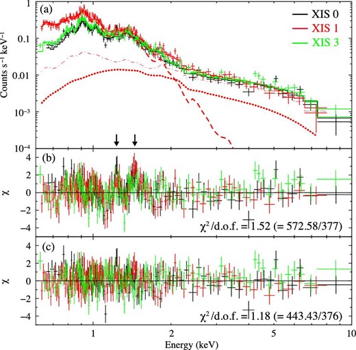
Top panel (a) shows spectra of the SW observation taken by the XIS 0 (black), 1 (red), and 3 (green). The solid curves are SW Model2. The dashed, dotted, and dash–dotted curves represent the VRNEI, the PL, and the background components of XIS 1, respectively. The lower two panels show the residuals of the data compared to SW Model1 (b), SW Model2 (c). The two arrows point at 1.23 keV and 1.45 keV, respectively. (Color online)
We first fitted the SW spectra with the same model as NE Model3 (hereafter SW Model1). The absorption column density of the CXB component estimated from the nh tool is 6.35 × 1021 cm−2. The best-fitting parameters and the residuals are shown in table 4 and figure 4b, respectively. The fit statistic is |$\chi ^2_\nu =1.52$|, and sawtooth-like residuals are shown around ∼1.23 keV and ∼1.45 keV. These energies correspond to the centroid energies of Fe L lines (e.g., Fe xxi 1s2 2s1 2p2 4s1→1s2 2s1 2p3 and Fe xxi 1s2 2s2 2p1 5d1→1s2 2s2 2p2), but these emissions are not strong in a plasma with kTe of ∼0.3 keV. In order to improve the residuals, we tried to add another plasma component with a high kTe because these Fe L lines have a peak at kTe ∼ 0.9 keV, but a suitable model could not be found.
Best-fitting parameters of the SW spectra.
| Model | Parameter (unit) | SW Model1 | SW Model2 |
|---|---|---|---|
| PHABS | N H (1021 cm−2) | 2.9 ± 0.4 | 4.5 ± 0.2 |
| VAPEC | kT e (keV) | |$0.298^{+0.008}_{-0.007}$| | 0.186|$^{+0.005}_{-0.004}$| |
| /VRNEI | kT init (keV) | — | 3.0 (fixed) |
| Z Ne (solar) | |$2.0^{+0.4}_{-0.3}$| | 2.9 ± 0.3 | |
| Z Mg (solar) | |$1.8^{+0.5}_{-0.4}$| | 1.0 ± 0.2 | |
| Z Si, S (solar) | <2.6 | 0.4 ± 0.2 | |
| Z Fe, Ni (solar) | |$0.43^{+0.07}_{-0.06}$| | |$2.1^{+0.3}_{-0.2}$| | |
| Z Others (solar) | 1.0 (fixed) | 1.0 (fixed) | |
| N* (1012 cm−5) | |$0.6^{+0.2}_{-0.1}$| | |$3.0^{+0.5}_{-0.4}$| | |
| n e t (1011 s cm−3) | — | 9.3 ± 0.4 | |
| PL | Γ | 3.5 ± 0.1 | 2.2 ± 0.3 |
| Surface brightness† | |$1.6^{+0.2}_{-0.1}$| | |$1.7^{+0.3}_{-0.2}$| | |
| χ2/d.o.f. | 572.58/377 | 443.43/376 |
*Normalization of the APEC component is |$\frac{1}{4\pi D^2} \int n_{\rm e}n_\mathrm{H}dV$|, where D is the distance to the source, ne and nH are the electron and hydrogen densities, respectively, and V is the X-ray emitting volume.
† Units of 10−15 erg cm−2 s−1 arcmin−2 in the 2.0–10.0 keV band.
Sawtooth-like residuals are often found in MM SNRs with RPs (e.g., Yamaguchi et al. 2009) because of a lack of radiative recombination continua (RRCs). The residuals around ∼1.23 keV and ∼1.45 keV indicate the excess of RRCs of He-like and H-like Ne, which are clear evidence of an RP. To investigate this hypothesis, we added two REDGE models to SW Model1. Figure 5 shows the result of the spectra fitting. We confirmed that the fit was significantly improved and the electron temperature of the REDGE models is |$0.13^{+0.04}_{-0.03}\:$|keV. The best-fitting energies of the REDGE models are 1.20 ± 0.02 keV and |$1.34^{+0.04}_{-0.03}\:$|keV, which are consistent with the edge energies of He-like and H-like Ne (1.196 keV and 1.362 keV), respectively.

The first (top) and third panels show spectra (red crosses) of the SW observation taken by XIS 1 with the best-fitting models (red solid lines). In the first panel, the model consists of the VAPEC (red dashed), PL (red dotted) and background (black dashed). In the third panel, the model is same as that in the top panel but it additionally includes two REDGE components with the edge energies of 1.189 keV (blue solid) and 1.34 keV (green solid). The second and fourth panels show the residuals of the data compared to the models. (Color online)
In order to apply an RP model to the full-band spectra, we used the VRNEI model, which takes into account ion fractions and ionization timescales of all elements in the recombination-dominant state. We therefore replace the VAPEC model to the VRNEI model and refer to this model as SW Model2. The VRNEI model calculates the spectrum of a non-equilibrium ionization plasma after a rapid transition of the electron temperature from kTinit to kTe with a recombining timescale (net). Since the initial temperature kTinit was not well constrained in our data, we fixed it to 3 keV, in which most Ne and Mg ions become bare nuclei. The best-fitting parameters and the residuals are shown in table 4 and figure 4c, respectively. No remarkable residuals are seen in SW Model2, and the fit statistic is significantly improved to |$\chi ^2_\nu =1.18$|. The obtained net = 9.3 × 10¹¹ s cm−3 indicates that the plasma in the SW region is indeed an RP.
3.2.4 Spatially resolved spectra
We found that the plasma in the NE region is in the CIE state while that in the SW region is in the recombining phase. In order to investigate more detailed spatial variation of the plasma properties, we divided the FoVs into five regions (A, B, C, D, and E), as shown in figure 1, according to the 0.6–2.0 keV morphology.
Regions A and B are included in the NE observation, and therefore we fitted their spectra with NE Model3. On the other hand, we applied SW Model2 to the spectra of regions C, D, and E, which are included in the SW observation. Since the non-functioning segment of XIS 0 occupies a large area in region E, we did not use the XIS 0 spectrum extracted from region E. We show the best-fitting parameters and the fitted spectra in table 5 and figure 6, respectively. All the spectra are well reproduced by the models. The photon index in region E is fixed at 2.2, which is the best-fitting value of the entire SW region, because that was not constrained in the fitting. We found significant spatial variations in NH, kTe, the metal abundances, and net.
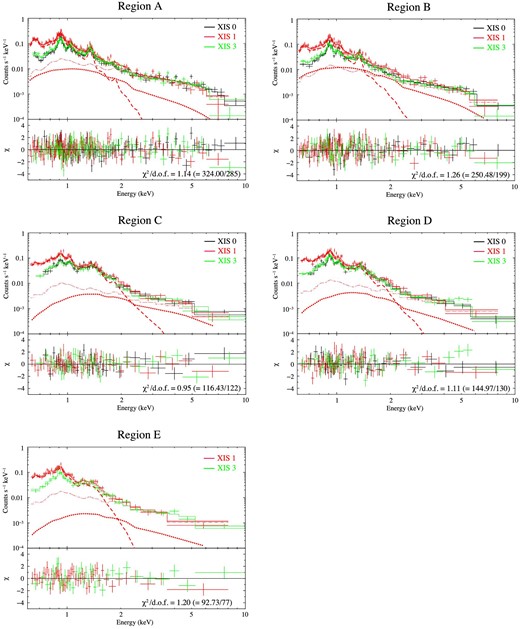
Each panel shows spectra extracted from each region taken by the XIS 0 (black), 1 (red), and 3 (green) and residuals from the best-fitting models. The solid curves are the best-fitting model. The dashed, dotted, and dash–dotted curves represent the VAPEC (regions A and B)/VRNEI (regions C, D, and E), the PL, and the background components of XIS 1, respectively. (Color online)
Best-fitting parameters of spectra for the spatial resolved analysis.
| Model | Parameter (unit) | Region A | Region B | Region C | Region D | Region E |
|---|---|---|---|---|---|---|
| Absorption | N H (1021 cm−2) | 2.3 ± 0.4 | 2.2 ± 0.5 | |$4.4^{+0.4}_{-0.5}$| | 4.4 ± 0.4 | |$4.3^{+0.5}_{-0.6}$| |
| VAPEC | kT e (keV) | |$0.288^{+0.007}_{-0.006}$| | |$0.306^{+0.010}_{-0.009}$| | |$0.193^{+0.010}_{-0.009}$| | 0.20 ± 0.01 | 0.155 ± 0.009 |
| /VRNEI | kT init (keV) | — | — | 3.0 (fixed) | 3.0 (fixed) | 3.0 (fixed) |
| Z Ne (solar) | |$1.9^{+0.3}_{-0.2}$| | |$2.4^{+0.5}_{-0.4}$| | |$2.9^{+0.6}_{-0.5}$| | |$2.7^{+0.5}_{-0.4}$| | |$3.2^{+0.9}_{-0.6}$| | |
| Z Mg (solar) | |$1.8^{+0.5}_{-0.3}$| | |$1.6^{+0.5}_{-0.4}$| | 0.8 ± 0.3 | |$1.3^{+0.4}_{-0.3}$| | <1.7 | |
| Z Si, S (solar) | <2.7 | <2.9 | 0.4 ± 0.2 | |$0.6^{+0.4}_{-0.5}$| | <4.0 | |
| Z Fe, Ni (solar) | 0.20 ± 0.03 | |$0.30^{+0.06}_{-0.05}$| | 1.4 ± 0.5 | |$1.2^{+0.6}_{-0.4}$| | >2.4 | |
| Z Others (solar) | 1.0 (fixed) | 1.0 (fixed) | 1.0 (fixed) | 1.0 (fixed) | 1.0 (fixed) | |
| N* (1012 cm−5) | 0.5 ± 0.1 | |$0.4^{+0.2}_{-0.1}$| | 3.3 ± 0.8 | |$2.7^{+0.8}_{-0.7}$| | |$2.6^{+1.1}_{-0.8}$| | |
| n e t (1011 s cm−3) | — | — | 7.0 ± 0.5 | |$9.9^{+0.8}_{-0.6}$| | 10.5 ± 1.0 | |
| PL | Γ | 2.7 ± 0.4 | 2.6 ± 0.2 | |$1.9^{+0.5}_{-0.6}$| | 2.6 ± 0.7 | 2.2 (fixed) |
| Surface brightness† | 0.8 ± 0.2 | 1.9 ± 0.3 | 2.5 ± 0.6 | 1.1 ± 0.3 | 0.7 ± 0.3 | |
| χ2/d.o.f. | 324.00/285 | 250.48/199 | 116.43/122 | 144.97/130 | 92.73/77 |
*Normalization of the APEC component is |$\frac{1}{4\pi D^2} \int n_{\rm e}n_\mathrm{H}dV$|, where D is the distance to the source, ne and nH are the electron and hydrogen densities, respectively, and V is the X-ray emitting volume.
† Units of 10−15 erg cm−2 s−1 arcmin−2 in the 2.0–10.0 keV band.
4 Discussion
4.1 Absorption column density toward CTB 1
From the spatially resolved analysis (sub-subsection 3.2.4), we obtained the absorption column densities of the five regions. The column densities of the inner radio-shell regions (regions C, D, and E) are about 2 times higher than those of the breakout regions (regions A and B). This result might indicate that there is a local enhancement of the ISM density around the radio shell of CTB 1. Indeed, the interaction between the CTB 1 shell and a surrounding H i gas was reported by Yar-Uyaniker, Uyaniker, and Kothes (2004). However, excess of a hydrogen column density estimated from the H i gas interacting with CTB 1 (TB ∼ 30 K at |$v$|LSR = −15.5–−18.5 km s−1) is 1.6 × 1020 cm−2, which is one order of magnitude smaller than that of our observations. A survey of 12CO (J = 1–0) in this area was performed by Heyer et al. (1998), but no association between CTB 1 and molecular clouds have been reported so far. Further observations of the cold ISM are necessary to identify the origin of the excess of the X-ray absorption column density at the shell of CTB 1.
We estimated the distance to CTB 1 according to the absorption column density toward the breakout region (NH ∼ 2.3 × 1021 cm−2). Assuming a mean interstellar hydrogen density of 1 cm−3, the distance is ∼0.8 kpc. This is the lowest value among estimation from other studies (1.6–3.1 kpc: Craig et al. 1997; Yar-Uyaniker et al. 2004). However, the mean interstellar hydrogen density toward the CTB1 direction is highly uncertain. If we adopt a hydrogen density of 0.4 cm−3, we obtained a distance of 2 kpc, which is an intermediate value of the previous estimates. In the following discussion, we assume a distance of 2 kpc. We confirmed that our conclusions are not affected even when the distance is changed within 0.8–3.1 kpc.
4.2 Recombining plasma in the SW region
Previous observations with Chandra and ASCA suggested that both the NE and SW plasmas of CTB 1 are in the CIE state with kTe of 0.2–0.3 keV (Lazendic & Slane 2006; Pannuti et al. 2010). However, our spectral analyses revealed that the SW plasma is not in CIE but in the recombining phase for the first time.
Previous studies of RPs indicate that it is effective for the investigation of the formation process of the RPs to compare the distributions of densities of ISM and the kTe values of the RPs (W 49 B: Lopez et al. 2013; IC 443: Matsumura et al. 2017a; W 28: Okon et al. 2018). Lopez et al. (2013) discussed that higher kTe values would be expected in a region with a high ambient gas density if they considered the rarefaction as the formation process of RPs. On the contrary, Matsumura et al. (2017a) and Okon et al. (2018) found that kTe of RPs in shock–cloud interaction regions is significantly lower than those in the other region, suggesting that the origin of the RPs is cooling by thermal conduction between the SNR plasma and the cool dense ISM.
CTB 1 provides a unique opportunity to test the formation process of the RP; its ambient density is low at the breakout region and high at the shell region (Yar-Uyaniker et al. 2004). As shown in figure 7, we found that kTe in the inner-shell region is lower than that in the breakout region. Moreover, the rim of the shell (region E) shows the lowest kTe. Therefore, the RP in CTB 1 is most likely explained by the thermal conduction scenario rather than the rarefaction scenario.
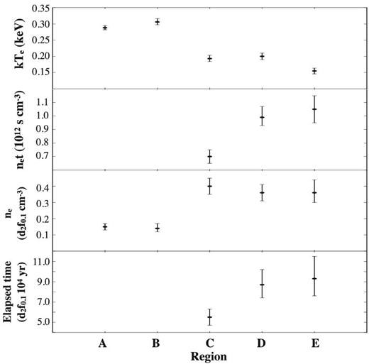
The first (top) panel shows electron temperatures in the regions A–E with a unit of keV. Second panel shows ionization parameters in the regions A–E with a unit of 1012 s cm−3. Third panel shows the densities of electrons. d2 is the distance to CTB 1 divided by 2 kpc and f0.1 is the filling factor divided by 0.1. The fourth panel shows elapsed times for each region.
In addition, we calculated the elapsed time since recombination started to dominate over ionization (trec) using net obtained from our spectral analyses. The bottom two panels of figure 7 show the electron densities (ne) estimated from the best-fitting emission measures and the derived trec for regions C, D, and E. The result suggests that the outer region became an RP earlier than the central region did. It is consistent with the thermal conduction scenario.
4.3 Spatial variation of the metal abundances
The abundances of Ne and Mg are larger than the solar values in both the NE and SW regions and are consistent with results of previous studies (Lazendic & Slane 2006; Pannuti et al. 2010). In contrast, we discover that the abundance of Fe in the SW region is much higher than that in the NE region. We note that the abundance of Fe is significantly affected by an assumed model as shown in a comparison between SW Model1 and SW Model2 (see table 4), and therefore precise modeling of the plasma ionization state is crucial to determine the metal abundances.
In figure 8, we plot a spatial variation in the abundance ratio of Ne to Fe. The ratios are systematically larger than unity, suggesting the origin of a core-collapse supernova (e.g., Nomoto et al. 2006; Takeuchi et al. 2016). In addition, the ratios in the inner-radio shell region are smaller than those in the breakout region. In particular, Fe is enhanced in region E. This indicates an asymmetric ejecta distribution as also found in other SNRs with the origin of core-collapse supernovae (e.g., Katsuda et al. 2008; Uchida et al. 2009). One of the possibilities is that Ne was isotropically ejected while Fe was ejected towards the SW.
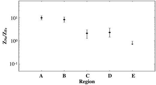
Abundance ratios of Ne to Fe in the regions A–E.
4.4 Origin of the hard-band excess
We found that the observed fluxes above 2 keV are larger than that of the CXB model by ∼13%–47% in both NE and SW. These hard-band excesses are represented by power-law functions. Photon indexes and surface brightnesses for all the regions are shown in figure 9. Γ is in the range of 2–3, and marginal spectral steeping is seen at the outer of CTB 1. On the other hand, the surface brightness has a peak at the center of the radio shell. A flux and a luminosity integrated over the observed regions are 4.5 × 10⁻¹³ erg s−1cm−2 and |$2.2\times 10^{32}d_{2}^2\:$|erg s−1 in the 2–10 keV band, respectively, where d2 is the distance to CTB 1 divided by 2 kpc. A spatial extent of the hard X-ray emission is 20d2 pc.
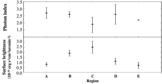
Top panel shows the photon index in the regions A–E. The photon index for the region E is fixed at the best-fitting value of the entire SW region (2.2). The lower panel shows the surface brightness (2.0–10 keV) in the regions A–E with a unit of 10−15 erg cm−2 s−1 arcmin−2.
Pannuti et al. (2010) reported the detection of power-law components in the NE and SW regions using ASCA spectra. The photon indexes and the fluxes they derived are consistent with those of our results. They also argued that a thermal plasma with kTe ∼ 3 keV, which might be a high-temperature plasma component in CTB 1, can explain the observed spectra instead of the power-law component. However, fitting a thermal plasma model to the Suzaku spectra (NE Model2) requires an extremely low abundance due to a lack of emission lines from He-like Fe. Because such a low abundance is not explained by either a supernova ejecta or the ISM, a high-temperature plasma associated with CTB 1 is unlikely.
One possible origin of the hard-band excess is a flux fluctuation of the CXB due to the cosmic variance. Indeed, an expected amplitude of the fluctuation for the Suzaku FoV is ∼15% (Moretti et al. 2009). In order to confirm the CXB fluctuation in the two background regions, we fitted the background spectra again with the free CXB normalizations, and found that the difference in the CXB normalizations between BG1 and BG2 is 14%, which is consistent with the above expectation. On the other hand, the hard-band excesses in CTB1 are 13%–47% of the CXB flux and are higher than the expected fluctuation in regions B, C, and D. Moreover, the derived photon index is significantly steeper than that of the CXB, and the excesses are observed in all regions. Therefore, it is unlikely that the origin of the hard-band excess is fluctuation in the CXB.
On the basis of the morphology, no clear association is seen between the X-ray hard-band excess and the radio shell. One possible origin is a pulsar wind nebula, because Γ, the luminosity, and the spatial extent is in the range of old Galactic pulsar wind nebulae (Kargaltsev et al. 2008; Bamba et al. 2010). According to the empirical relation between the luminosity and the characteristic age (Mattana et al. 2009), the characteristic age is 104–105 yr, which is consistent with the age of CTB 1. The spin-down luminosity of the pulsar is estimated to be 2.8 × 1035 erg s−1 assuming |$L_\mathrm{x}/\dot{E}_\mathrm{rot} = 8\times 10^{-5}$| for old pulsar wind nebulae (Vink et al. 2011). However, no pulsar has been detected at the center of CTB 1. Moreover, gamma-ray emission from a pulsar wind nebula has not been detected so far even though the expected TeV gamma-ray luminosity is ∼102Lx, according to the relation shown by Mattana et al. (2009). Further multi-wavelength observations are necessary to examine this scenario.
5 Summary
We observed MM SNR CTB 1 with Suzaku for a total exposure of ∼82 ks, and obtained the following results from the spectral analysis.
The 0.6–2.0 keV spectra in the NE breakout region of CTB 1 were fitted with a CIE plasma model with kTe ∼ 0.3 keV, whereas those in the SW inner-shell region were well represented by an RP model with kTe ∼ 0.19 keV, kTinit = 3.0 keV, and net ∼ 9 × 1011 cm−3 s. This is the first detection of an RP in CTB 1.
The characteristic morphology of CTB 1 provides unique opportunity to test the formation scenarios of RPs. Our results show that kTe in the inner-shell region is lower than that in the breakout region, and becomes lowest at the rim of the shell. In addition, trec increases toward the outer region. Therefore, the thermal conduction scenario is likely for the formation of the RP in CTB 1 rather than the rarefaction scenario.
The Ne abundance is almost uniform in the observed regions, whereas the Fe abundance is enhanced in the inner-shell region, suggesting the asymmetric ejecta distribution.
The diffuse hard X-ray emission represented by a power-law function is detected. The photon index is ∼2.5 and the total flux is ∼5 × 10⁻¹³ erg cm−2 s−1 in the 2–10 keV band. The surface brightness is peaked at the center of CTB 1. The origin of this emission is an open question but one possibility is a pulsar wind nebula associated with this remnant.
Acknowledgments
We appreciate all the Suzaku team members. This work is supported by Japan Society for the Promotion of Science (JSPS) KAKENHI grant number 16J02332 (M.K.), 18J01417 (H.M.), 16H02170(T.T.) and the World Premier International Research Center Initiative (WPI), MEXT, Japan. S.N. is supported by the RIKEN Special Postdoctoral Researcher Program. S.-H.L. is supported by The Kyoto University Foundation (grant no. 203180500017). M.A. is supported by the RIKEN Junior Research Associate Program.
Footnotes
References
