


Abstract
We present Nobeyama 45 m telescope C18O, 13CO, and 12CO(1–0) mapping observations towards an interstellar filament in the Taurus molecular cloud. We investigate the gas velocity structure along the filament and in its surrounding parent cloud. The filament is detected in the optically thin C18O emission as a single velocity component with a ∼1 pc long, ∼0.06 pc wide structure. The C18O emission traces dust column densities larger than ∼5 × 1021 cm−2. The line-of-sight (LOS) velocity fluctuates along the filament crest with an average amplitude of ∼0.2 km s−1. The 13CO and 12CO integrated intensity maps show spatially extended emission around the elongated filament. We identify three extended structures with LOS velocities redshifted and blueshifted with respect to the average velocity of the filament identified in C18O. Based on combined analyses of velocity-integrated channel maps and intensity variations of the optically thick 12CO spectra on and off the filament, we propose a three-dimensional structure of the cloud surrounding the filament. We further suggest a multi-interaction scenario where sheet-like extended structures interact, in space and time, with the filament and are responsible for its compression and/or disruption, playing an important role in the star formation history of the filament. We also identify, towards the same field, a very faint filament showing a velocity field compatible with the filament formation process proposed by Inoue et al. (2018, PASJ, 70, S53), where a filament is formed due to convergence of a flow of matter generated by the bending of the ambient magnetic field structure induced by an interstellar shock compression.
1 Introduction
Molecular clouds are observed to be filamentary (e.g., André et al. 2010; Molinari et al. 2010; Umemoto et al. 2017). Filamentary molecular clouds are proposed to be formed out of dense and cold atomic clouds as a result of multiple compressions from propagating shock waves through the interstellar medium (e.g., Hennebelle et al. 2008; Inoue & Inutsuka 2009; Inutsuka et al. 2015). The typical timescale of such shock compressions is estimated to be on average ∼1 Myr (McKee & Ostriker 1977). After each passage of a wave, the properties of the shocked molecular interstellar medium (ISM) are modified. Thus, the present morphologies of the density, velocity, and magnetic field structures are usually not those corresponding to the initial conditions at the molecular cloud formation epoch, but are probably the result of their sequential alteration due to interactions with multiple propagating ISM waves.
Hence, in order to describe the formation and evolution of structures in molecular clouds, one should take into account the reorganization of interstellar matter, as a function of time, due to the propagation of waves through the filamentary clouds.
In the context of star formation, these propagating shock waves may as a consequence be responsible for the assembly of dense molecular matter in the form of “thermally supercritical” filaments where the bulk of star formation is observed to take place (e.g., André et al. 2010; Könyves et al. 2015; Marsh et al. 2016). These thermally supercritical filaments are characterized with a mass per unit length, Mline, of the order of or larger than the critical line mass of nearly isothermal, long cylinders, |$M_{\rm line,crit}=2 c_{\rm s}^{2}/G \sim 16\, M_{\odot }\, \rm pc^{-1}$| (Stodólkiewicz 1963; Ostriker 1964) where cs ∼ 0.2 km s−1 for a gas temperature of ∼10 K, and are unstable for radial collapse and fragmentation (cf. Inutsuka & Miyama 1997). This critical mass per unit length corresponds to a column density of |$N_{\rm H_{2}}\sim 8\times 10^{21}\,$|cm−2 or a surface density of |$\Sigma _{\rm fil}^0\sim 116\, M_{\odot } \, {\rm pc}^{-2}$| for 0.1 pc-wide filaments (Arzoumanian et al. 2011). These latter values are comparable to the proposed column density threshold for star formation (Lada et al. 2010; Shimajiri et al. 2017). Hence, the column density threshold for star formation can now be understood as the threshold in filament Mline equivalent to a critical value of hydrostatical equilibrium above which filaments are unstable to radial collapse and fragmentation into star-forming cores (cf. André et al. 2014).
The analyses of Herschel observations towards the Aquila star-forming region suggest that a relatively small fraction, about 15% on average, of the mass of supercritical filaments is in the form of prestellar cores (Könyves et al. 2015). Understanding this observed fraction, in the light of star formation along supercritical filaments, may give us a hint on the origin of the observed star formation efficiency in molecular clouds and in the Galaxy.
Molecular filaments are observed to span a wide range in central column density, mass per unit length, and length, while they all share the same central width of about 0.1 pc (as derived in nearby regions from Herschel dust continuum observations; Arzoumanian et al. 2011, 2018; Juvela et al. 2012; Alves de Oliveira et al. 2014; Koch & Rosolowsky 2015, and others). The origin of this filament property is not yet understood. Arzoumanian et al. (2011) suggested that the characteristic filament width may be linked to the sonic scale of turbulence in the cold (∼10 K) ISM, observed to be around 0.1 pc (Larson 1981; Goodman et al. 1998). The latter appears to be roughly the scale at which supersonic magnetohydrodynamic (MHD) turbulence dissipates (Vázquez-Semadeni et al. 2003; Federrath et al. 2010), compatible with the observed subsonic to transonic velocity dispersions of subcritical/critical filaments (Arzoumanian et al. 2013; Hacar et al. 2013, 2016). These results suggest that the dissipation of large-scale shock waves in the ISM may be important for the formation of the observed filamentary web (Inutsuka et al. 2015; Inoue et al. 2018).
In this paper we present Nobeyama 45 m telescope C18O(1–0), 13CO(1–0), and 12CO(1–0) molecular line observations towards a prominent ∼1 pc-long filament identified with Herschel in the Taurus molecular cloud (figure 1). In section 2 we present our mapping observations with the Nobeyama 45 m telescope. Section 3 details the results derived from analysis of the velocity cubes, the spectra, the channel maps, and the position–velocity maps along, across, and around the filament. In section 4 we discuss the implications of our results in the understanding of filament formation, evolution, and interaction with the surrounding cloud. We summarize the results presented in this paper and conclude in section 5. Three appendices complement the analyses presented in the main text.
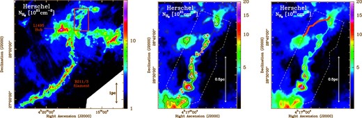
Left: Column density map of part of the Taurus molecular cloud as derived from Herschel Gould Belt Survey Archive data1 (cf. Palmeirim et al. 2013). The B211/3 well-studied filament and the L1495 star-forming hub are indicated. The red rectangle shows the region analyzed in this paper. Middle: Blow-up column density map, at the resolution of 28″, of the red rectangle plotted in the left panel. The black contours are at column densities of 4, 6, and 8 × 1021cm−2. The blue- and red-white triangles are the prestellar cores and the unbound fragments identified by Marsh et al. (2016), respectively. The white dashed contour shows the footprint of the CO maps observed with the Nobeyama 45 m telescope. Right: The map is the same as the middle panel. The blue and red skeletons trace the crests of the two filaments discussed in this paper, MF and YF, respectively. (Color online)
2 Molecular line mapping observations with the Nobeyama 45 m telescope
We used the Nobeyama 45 m telescope to map a molecular filament previously identified by Herschel and its surrounding parent cloud (see figure 1). The target region is located on the west of the star-forming L1495 hub in the Taurus molecular clouds at a distance of 140 pc (Elias 1978; Myers 2009; Ward-Thompson et al. 2016). The observations were carried out in 2017 February. We mapped a 0.14 deg2 region around the filament in 12CO(1–0), 13CO(1–0), and C18O(1–0) with the FOREST receiver (Minamidani et al. 2016). All molecular line data were obtained simultaneously. At 115 GHz, the telescope has a beam size of ∼15″ (HPBW). As backend, we used the SAM45 spectrometer which provides a bandwidth of 31 MHz and a frequency resolution of 7.63 kHz. The latter corresponds to a velocity resolution of ∼0.02 km s−1 at 115 GHz. The standard chopper wheel method was used to convert the observed signal to the antenna temperature |$T_{\rm A}^*$| in units of K, corrected for the atmospheric attenuation. To estimate the main beam brightness temperature, TMB, we mapped a small area of the OMC-2/FIR 4 region with strong dust continuum emission in the OMC-2/3 region (Shimajiri et al. 2008, 2015a, 2015b) once or twice per observing day. We scaled the FOREST intensity (|$T_{\rm A}^*$|) to the intensity of the BEARS data (TMB) obtained in Shimajiri et al. (2011, 2014) by comparing the FOREST intensity with the BEARS intensity in the OMC-2/FIR 4 region. During the observations, the system noise temperatures ranged from 150 K to 580 K. The telescope pointing was checked every hour by observing the SiO maser source NML-tau, and was better than 3′ throughout the entire observing run. We used the on-the-fly (OTF) mapping technique. The central position of our final map is (RAJ2000.0, DecJ2000.0) = (|${04^{\rm h}16^{\rm m}49{^{\rm s}_{.}}711}$|, 28°|${35^{\prime }42{^{\prime\prime}_{.}}35}$|). We have chosen lines of sight of (RAJ2000.0, DecJ2000.0) = (|${04^{\rm h}11^{\rm m}48{^{\rm s}_{.}}691}$|, 26°|${46^{\prime }25{^{\prime\prime}_{.}}59}$|) as the off position for baseline removal. We obtained OTF maps with two different scanning directions along the RA and Dec axes and combined them into a single map using the Emerson and Graeve (1988) PLAIT algorithm to reduce the scanning effects. We then smoothed spatially and spectrally all three cubes to the same effective HPBW size of 28″ and velocity resolution of 0.07 km s−1. The 1 σ noise level of the final data at 28″ and 0.07 km s−1 are 0.48 K, 0.22 K, and 0.20 K in TMB for 12CO(1–0), 13CO(1–0), and C18O(1–0), respectively.
3 Analyses and results
3.1 Integrated intensity maps of 12CO(1–0), 13CO(1–0), and C18O(1–0)
We derived velocity-integrated intensity maps for the three lines of the observed region (figure 2). The emission is integrated for the local standard of rest (LSR) velocity range between 4 and 9 km s−1, which encompasses the bulk of the emission of the observed region, as can be seen on the 12CO(1–0), 13CO(1–0), and C18O(1–0) spectra averaged across the whole field (figure 3).
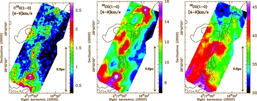
From left to right, C18O(1–0), 13CO(1–0), and 12CO(1–0) integrated intensity maps (in units of K km s−1) over the LSR velocity range 4 to 9 km s−1. The spatial and spectral resolutions of the maps are 28″ and 0.07 km s−1, respectively. The black contours correspond to column densities of 4, 6, and 8 × 1021cm−2 derived from Herschel data, and are the same as those in figure 1. The C18O(1–0) integrated emission traces the elongated structure of the filament. (Color online)
![Positionally averaged spectra (across the whole observed region) of 12CO(1–0), 13CO(1–0), and C18O(1–0) emissions. The 13CO and C18O spectra are multiplied by a factor 2 and 10, respectively. The five colored vertical rectangles show the five velocity channels, which we use to divide the total integrated emission based on position–velocity diagrams as explained in subsection 3.2. The five channels are as follows: B[4–5.4] km s−1, F1[5.4–6.2] km s−1, R1[6.2–7.2] km s−1, R2[7.2–8.1] km s−1, F2[8.1–8.7] km s−1. (Color online)](https://oup.silverchair-cdn.com/oup/backfile/Content_public/Journal/pasj/70/5/10.1093_pasj_psy095/3/m_pasj_70_5_96_f10.jpeg?Expires=1749203342&Signature=gcDYqcyQtvYbHNe8TRU26ajI6FL52r7UmelUuAl5g3l3NQpu3kZPUKBKeIR0GIdS~peG3MXf2m26FXKtjwNJE1J05Y1~sVpER44WggSbqms1XjihUUMZhNQNXM14zHlJ-AsH0yLYTdvJjWNSJRuicY8J1loZrOLIbMkbgIkz6vQ8~Satv6UtJSb-FLS8SGgCOuAl-uY~o4m0IFk1l0dUqdDq1DzzwQYVede~PSMrymF6oTc1e7SxMXKkwLLzgPPA36gzHAGALwpYKuX30juh0dqBNvbG3igfB1MltdvBIqUhsFU5RPgPrvlOie1lMJHuj~kkqgDzpU~OWE~oSXZy2g__&Key-Pair-Id=APKAIE5G5CRDK6RD3PGA)
Positionally averaged spectra (across the whole observed region) of 12CO(1–0), 13CO(1–0), and C18O(1–0) emissions. The 13CO and C18O spectra are multiplied by a factor 2 and 10, respectively. The five colored vertical rectangles show the five velocity channels, which we use to divide the total integrated emission based on position–velocity diagrams as explained in subsection 3.2. The five channels are as follows: B[4–5.4] km s−1, F1[5.4–6.2] km s−1, R1[6.2–7.2] km s−1, R2[7.2–8.1] km s−1, F2[8.1–8.7] km s−1. (Color online)
The C18O(1–0) integrated emission traces the elongated structure of the filament (figure 2) with column densities |$N_{\rm H_{2}}\gtrsim 5 \times 10^{21}\, {\rm \, cm^{-2}}$| as derived from Herschel data (figure 1; see also appendix 1). The 13CO and 12CO integrated intensity maps show more extended emission around the filament for column densities |$N_{\rm H_{2}}\gtrsim 1 \times 10^{21}\, {\rm \, cm^{-2}}$|. In the following we refer to the filament identified with Herschel and traced with the C18O(1–0) emission as the main filament, MF. The filament MF can hardly be recognized in the velocity-integrated map of the 13CO emission and cannot be seen in the 12CO emission map (figure 2).
We derive 12CO(1–0)|$/$|13CO(1–0) and 13CO(1–0)|$/$|C18O(1–0) ratio maps from the velocity-integrated maps over the LSR velocity range 4 to 8.7 km s−1 (figure 4) to estimate the mean optical depth of the three lines (see, e.g., section 4 of Arzoumanian et al. 2013). The mean optical depth values of the 12CO(1–0), 13CO(1–0), and C18O(1–0) lines for the integrated emission are estimated to be in the ranges |$12 < \tau _{^{12}\rm {CO}} < 39$|, |$0.06 < \tau _{^{13}\rm {CO}} < 0.9$|, and |$0.01 < \tau _{\rm {C}^{18}\rm {O}} <0.15$|, respectively, assuming mean values of the abundance ratios [12CO]|$/$|[13CO] = 62 (Langer & Penzias 1993) and [13CO]|$/$|[C18O] = 5.5 (Wilson & Rood 1994) in the local ISM (see also table 1). The 12CO(1–0) emission is found to be highly optically thick over the entire observed field, while the C18O(1–0) and 13CO(1–0) emissions are mostly optically thin. Table 1 gives the optical depth values for the five channel maps derived by integrating the emission over smaller velocity ranges corresponding to the five identified emission structures with different velocity components. While the C18O emission is optically thin for all channels, the 13CO emission is estimated to be locally slightly optically thick (cf. subsection 3.2 and table 1).
![Integrated intensity ratio map $\int _{4}^{9}T_{\rm MB}^{12}(\upsilon ){d}{\it \upsilon } / \int _{4}^{9} T_{\rm MB}^{13}({\it \upsilon } ){d}{\it \upsilon }$ (left) and $\int _{4}^{9}T_{\rm MB}^{13}(\upsilon ){d}{\it \upsilon } / \int _{4}^{9} T_{\rm MB}^{18}({\it \upsilon } )d{\it \upsilon }$ (right). The $T_{\rm MB}^{12}$, $T_{\rm MB}^{13}$, and $T_{\rm MB}^{18}$ correspond to the mean beam brightness temperature of the 12CO(1–0), 13CO(1–0), and C18O(1–0) emissions, respectively, $\upsilon$ is the line-of-sight velocity in the range [4–9] km s−1. The integrated intensity maps are the same as in figure 2. For the right-hand side map, only pixels with $T_{\rm MB}^{18}>5\, \sigma$ have been considered, where σ = 0.2 K (section 2). The 12CO(1–0) emission is optically thick over the entire observed field. The C18O(1–0) and 13CO(1–0) emissions are optically thin. (Color online)](https://oup.silverchair-cdn.com/oup/backfile/Content_public/Journal/pasj/70/5/10.1093_pasj_psy095/3/m_pasj_70_5_96_f11.jpeg?Expires=1749203342&Signature=3m~kWeBOerpBdS-0r8s3dgBi1aesjw7crjNsGx1i0noBDZKbrm~p3d4sXjlQo2CCesBcdoI1cEwKbuRNMIVHINO-wurPdo9hT7wxtFlgsKV3FVTH3rk8YSmPmtPvzJ2wgTbDP5bIWg0oD6yh71Np4n7iqvzJD33dWDqQDXjcE436IM7LtZEreJCKAUeY1TkHx9xZQvhKabOY-UjV15iT0OT9-Vm8HzeOxaaOFWUJj73~ls0NvAnLvFm0uRmSn4c9pVOt-xp8gi86AzRNbWTVzgIpiJUGLZN67B5HmgG3mfaLNVmsiWhTK1oFxYdmSFqiaQSLItJ9~Uh-e8k6hq4YCg__&Key-Pair-Id=APKAIE5G5CRDK6RD3PGA)
Integrated intensity ratio map |$\int _{4}^{9}T_{\rm MB}^{12}(\upsilon ){d}{\it \upsilon } / \int _{4}^{9} T_{\rm MB}^{13}({\it \upsilon } ){d}{\it \upsilon }$| (left) and |$\int _{4}^{9}T_{\rm MB}^{13}(\upsilon ){d}{\it \upsilon } / \int _{4}^{9} T_{\rm MB}^{18}({\it \upsilon } )d{\it \upsilon }$| (right). The |$T_{\rm MB}^{12}$|, |$T_{\rm MB}^{13}$|, and |$T_{\rm MB}^{18}$| correspond to the mean beam brightness temperature of the 12CO(1–0), 13CO(1–0), and C18O(1–0) emissions, respectively, |$\upsilon$| is the line-of-sight velocity in the range [4–9] km s−1. The integrated intensity maps are the same as in figure 2. For the right-hand side map, only pixels with |$T_{\rm MB}^{18}>5\, \sigma$| have been considered, where σ = 0.2 K (section 2). The 12CO(1–0) emission is optically thick over the entire observed field. The C18O(1–0) and 13CO(1–0) emissions are optically thin. (Color online)
Median values of optical depth, column density, and line-of-sight length for the different structures identified in velocity space.*
| Structure | Velocity range | |$\tau _{^{13}\rm {CO}}$| | |$\mathit {FWHM}_{^{13}\rm {CO}}$| | 13 |$N_{\rm H_{2}}$| | 13 l LOS | |$\tau _{\rm {C}^{18}\rm {O}}$| | |$\mathit {FWHM}_{\rm {C}^{18}\rm {O}}$| | |$^{18}N_{\rm H_{2}}$| | 18 l LOS |
|---|---|---|---|---|---|---|---|---|---|
| [ km s−1] | [ km s−1] | [1021|$\rm \, cm^{-2}$| ] | [pc] | [ km s−1] | [1021|$\rm \, cm^{-2}$| ] | [pc] | |||
| (1) | (2) | (3) | (4) | (5) | (6) | (7) | (8) | (9) | (10) |
| SB | B[4–5.4] | 0.80 | 0.68 | 1.73 | 0.28 | 0.15 | 0.70 | 3.82 | 0.25 |
| MF | F1[5.4–6.2] | 0.75 | 0.51 | 1.31 | 0.21 | 0.20 | 0.44 | 3.06 | 0.20 |
| SR1 | R1[6.2–7.2] | 0.79 | 0.68 | 1.76 | 0.29 | 0.21 | 0.58 | 4.35 | 0.28 |
| SR2 | R2[7.2–8.1] | 1.09 | 0.66 | 2.45 | 0.40 | 0.16 | 0.47 | 2.80 | 0.18 |
| YF | F2[8.1–8.7] | 0.67 | 0.42 | 0.97 | 0.16 | 0.14 | 0.40 | 1.98 | 0.13 |
| All† | 0.79 | 0.66 | 1.73 | 0.28 | 0.16 | 0.47 | 3.06 | 0.20 |
*The median values are computed over the observed field, for each velocity range, and for a signal-to-noise ratio |$\mathit {SNR}>5$|. (1) Name of the structure identified in the given velocity range. (2) Velocity range identified from the PV diagrams (see figure 5 and subsection 3.2). (3) Optical depth of the |$^{13}\rm {CO}$| emission calculated using equation (1) from Shimajiri et al. (2014), assuming an excitation temperature of 10 K in local thermodynamic equilibrium (LTE) conditions, and a filling factor of 1. The peak brightness temperature of the |$^{13}\rm {CO}$| emission over the observed region has been derived using the MOMENT task in MIRIAD for each velocity range. (4) |$\mathit {FWHM}$| line width of the |$^{13}\rm {CO}$| spectra derived using the MOMENT task in MIRIAD for each velocity range. (5) H2 molecular gas column density derived from |$^{13}\rm {CO}$| column densities calculated using equation (2) from Shimajiri et al. (2014), assuming a fractional abundance of |$^{13}\rm {CO}$| with respect to H2 of 1.7 × 10⁻⁶ (Frerking et al. 1982). (6) Extent of the emitting structure along the line of sight estimated from the column density given in (5) for a critical density of 2 × 103 cm−3. (7) to (10) Same as (3) to (6) for the C18O emission, with a fractional abundance of C18O with respect to H2 of 1.7 × 10⁻⁷ and a critical density of 5 × 103 cm−3.
†Median values for the five structures.
3.2 Position–velocity diagrams and channel maps
Figure 5 shows position–velocity (PV) diagrams perpendicular to the main axis of the filament MF, and averaged along its length. In practice, the cubes have first been rotated by 25° (corresponding to the mean orientation of MF on the plane of the sky) from north to east. Second, the PV-cuts in the horizontal direction have been averaged in the vertical direction along the 1 pc length of the filament. Averaging the emission increases the signal-to-noise ratio (SNR), which makes it possible to detect extended C18O(1–0) emission which is not strong enough to be detected otherwise, e.g., on the channel maps (figures 6 and 7).
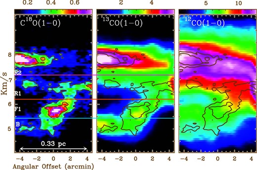
Position–velocity diagrams, in units of K(TMB), of the C18O(1–0), 13CO(1–0), and 12CO(1–0) emissions, from left to right. These PV diagrams are perpendicular to the MF filament axis and averaged along its crest. The zero-offset position (on the x-axis) indicates the position of the filament. The black contours correspond to the C18O(1–0) intensity at 0.3 and 0.5 K, and are the same for the three panels. The three horizontal lines in blue, red, and purple show velocities of 5.4, 6.2, and 7.2 km s−1, respectively. These lines identify the four velocity ranges, B, F1, R1, and R2 described in subsection 3.2. (Color online)
![Velocity channel maps in units of K km s−1. From left to right, velocity-integrated intensity maps for 12CO(1–0), 13CO(1–0), and C18O(1–0) emissions. From top to bottom, channel maps derived by integrating the intensity for the following velocity ranges: B[4–5.4] km s−1, F1[5.4–6.2] km s−1, and R1[6.2–7.2] km s−1. The velocity ranges of the channel maps are indicated on the top left of each panel. The spatial and spectral resolutions of the maps are 28″ and 0.07 km s−1, respectively. The blue contours correspond to column densities of 4, 6, and 8 × 1021cm−2 derived from Herschel data, and are the same as those in figure 1. Note that the range of the color scale (indicated by the bar in the top of each panel) is different for each plot. This scale has been chosen to represent the dynamical range of the emission for each velocity channel map. (Color online)](https://oup.silverchair-cdn.com/oup/backfile/Content_public/Journal/pasj/70/5/10.1093_pasj_psy095/3/m_pasj_70_5_96_f13.jpeg?Expires=1749203342&Signature=dfC7nHEe6heMJnh6H~u5Do42ZWUcGIPzuM2qHIU5RL1YPBrAw0ERUMhi1LuL1eCi~rwAe1KV0SSqma0L1YkQOitLfIoylpMyzp0sgeZMC68WgwX23wDAwfxP~my7QtNb6ID7Bh8D1QV774l9-54LRXgjzueWyN97qgZtEiKljP7faK-et-lUc8VL75jD8EbV1FkfLN5XTp8I8xd2Ch-B~KR0lPYql5VtWhEJqaAQX-0HgJcAHUNuUL49yrgk5kkYWfnks9W76rznwPKcdspBtOee0kTadXQUSIiKamaDqQgHT1n~n~eLY0uYXzw5LZchDrHToB8YzaeSOX02QLX4OQ__&Key-Pair-Id=APKAIE5G5CRDK6RD3PGA)
Velocity channel maps in units of K km s−1. From left to right, velocity-integrated intensity maps for 12CO(1–0), 13CO(1–0), and C18O(1–0) emissions. From top to bottom, channel maps derived by integrating the intensity for the following velocity ranges: B[4–5.4] km s−1, F1[5.4–6.2] km s−1, and R1[6.2–7.2] km s−1. The velocity ranges of the channel maps are indicated on the top left of each panel. The spatial and spectral resolutions of the maps are 28″ and 0.07 km s−1, respectively. The blue contours correspond to column densities of 4, 6, and 8 × 1021cm−2 derived from Herschel data, and are the same as those in figure 1. Note that the range of the color scale (indicated by the bar in the top of each panel) is different for each plot. This scale has been chosen to represent the dynamical range of the emission for each velocity channel map. (Color online)
![As figure 6, where the channel maps are derived by integrating the intensity for the velocity ranges of R2[7.2–8.1] km s−1 (top) and F2[8.1–8.7] km s−1 (bottom). The green squares on the bottom middle panel indicate the 2′ × 2′ squares used to average the 12CO(1–0) spectra plotted in figure 9 and discussed in subsection 3.3. The blue oblique segment on the northeast of the field, with an orientation of 30° (from north to east), shows the perpendicular direction to the YF filament used to derive the PV diagrams of figure 8. The length of the segment corresponds to 5 (${2{^{\prime}_{.}}5}$ on either side of the filament crest). (Color online)](https://oup.silverchair-cdn.com/oup/backfile/Content_public/Journal/pasj/70/5/10.1093_pasj_psy095/3/m_pasj_70_5_96_f14.jpeg?Expires=1749203342&Signature=RohVmzzWM9cPZ7tBgrnBKaSDIlXKZmtZy5SyoEI-RxBOfOtYvVf6kC8eu~bm4EkrpwNQ1Tf4n1Y8mA-lv5nR2OW4l9qF6N0YTC9BbNLSsrfbq85R0OjC3n~~U5OhLtpM~d6dw~nH2DAUj6s45u7YlzunzcokNVVa2RSbjOicbEH7W7NURtIlDRhT7Khz7GdG0xjuOsoiQ2rasZRPvWc9J40xhrO8WLaBIOlS2~U3~hqOafldGG1amqdFqwlc13ppaHMmXvH7yiVcD9xcxaLFW9k19bLztTT5AeV6WAoXBf80-QHErfs~yyYQ4nkQ8mVL6YvzJHS0au~eaLIHOkrYWw__&Key-Pair-Id=APKAIE5G5CRDK6RD3PGA)
As figure 6, where the channel maps are derived by integrating the intensity for the velocity ranges of R2[7.2–8.1] km s−1 (top) and F2[8.1–8.7] km s−1 (bottom). The green squares on the bottom middle panel indicate the 2′ × 2′ squares used to average the 12CO(1–0) spectra plotted in figure 9 and discussed in subsection 3.3. The blue oblique segment on the northeast of the field, with an orientation of 30° (from north to east), shows the perpendicular direction to the YF filament used to derive the PV diagrams of figure 8. The length of the segment corresponds to 5 (|${2{^{\prime}_{.}}5}$| on either side of the filament crest). (Color online)
These PV diagrams show multiple velocity components towards the filament MF and its surroundings. From the C18O(1–0) mean PV diagram, we identify four velocity components: B[4–5.4] km s−1, F1[5.4–6.2] km s−1, R1[6.2–7.2] km s−1, and R2[7.2–8.1] km s−1. The velocities given in the brackets correspond to the velocity ranges considered for each of the four components. The F1 velocity range corresponds to that of the filament MF (cf. subsection 3.4 and figure 6). A fifth velocity component, F2[8.1–8.7] km s−1, is identified on the 13CO(1–0) channel map, as can be seen in figure 7 (bottom middle panel).
The analysis of the 12CO(1–0) and 13CO(1–0) velocity cubes indicates that the gas structures emitting at the velocity ranges B, R1, and R2 introduced above have different spatial distributions towards and around MF. We name as SB, SR1, and SR2 the structures associated with the velocity ranges B, R1, and R2, respectively. In the following, we describe the spatial distributions of these different emitting structures that can be seen on the channel maps of figures 6 and 7.
As already mentioned, the filament MF is traced in C18O(1–0) at the velocity range F1, while at this same velocity range, the 12CO emission shows an extended emission around MF, with some decrease of the intensity towards the filament crest (see also subsection 3.3). Similarly, the 13CO emission, albeit tracing MF, has a more extended structure on both sides of the filament crest. The 13CO emission of the SB structure, associated with the B velocity range, is mostly located on the eastern part of MF, while the 12CO emission is also partly detected on the western side of MF. SR1 is mostly traced towards the south and northwest of the field in both 12CO and 13CO. SR2 covers mostly the northern part of the field in 13CO, while the 12CO emission is also seen in the south. At velocities in the range F2[8.1–8.7] km s−1, a second filament appears very bright in the northeast part of the field (see the bottom middle panel of figure 7). We identify this filament as YF (young filament; see subsection 4.2 and figure 1).
The three extended structures, SB, SR1, and SR2, identified from the PV diagram of the C18O emission do not have sharp boundaries in space and in velocity but are interconnected spatially with continuous velocity fields. We can seen on figure 5 velocity gradients across MF from the B to the R1 velocity ranges, traced by both the C18O and the 13CO emissions. These velocity bridges suggest that both structures, SB and SR1, may be physically connected to MF with partly mixed velocities. On the other hand, SR2 may not be presently directly connected to MF either in velocity nor probably in space.
The PV diagrams perpendicular to YF (figure 8) show two extended structures, one at velocities ∼5 km s−1 and another at ∼8 km s−1. These two velocity components correspond to the channels B and R2, respectively (see figure 8). The filament YF is identified on these PV diagrams in both C18O(1–0) and 13CO(1–0) as a compact structure at a velocity ∼8.3 km s−1. On the 12CO(1–0) PV diagram an extended structure is detected at velocities between ∼7.5 and 8.5 km s−1, with a bend around the position of YF (figure 8; see subsection 4.2).
![Position–velocity diagrams, in units of K(TMB), of C18O, 13CO, and 12CO, from left to right. These PV diagrams are constructed by averaging all the cuts taken perpendicular to the axis of YF as traced in the 13CO emission integrated over F2[8.1–8.7] km s−1 (see the bottom middle panel of figure 7). The zero-offset position (on the x-axis) indicates the position of YF. The contours correspond to the 13CO emission and are the same on the three panels. (Color online)](https://oup.silverchair-cdn.com/oup/backfile/Content_public/Journal/pasj/70/5/10.1093_pasj_psy095/3/m_pasj_70_5_96_f15.jpeg?Expires=1749203342&Signature=03fAfiVEz0sjlNEOqxeCJtoydLBeNc4M-c6B8k5szFNgmmgmnnrJKRpSggfo5PrFZw6Wy4EHNPdFnkeuJCRGEv8EmDmjWp8Lke4J~EKW2ulyBtNIa0pVExMF-8p5TZOQ3VuYuV1Qa9WkevZd6vIVC-pYqDcO6jZMCOO3ohfmST0UsMFjHZ5GC2BY01941FDwJpILM7ShTKuaaJBFVhePUvLHv74STSzAo8j22XnBnH7LdHI1nTNJ-a0Gob~jaVpR45~20mloB9Ux4cQ9zRn1~WCncB9VxoqmzCenbfFSVvmwX7K-3I-ozZHGtlRQt1YSBoporoNBUW9Rhaibc1orVw__&Key-Pair-Id=APKAIE5G5CRDK6RD3PGA)
Position–velocity diagrams, in units of K(TMB), of C18O, 13CO, and 12CO, from left to right. These PV diagrams are constructed by averaging all the cuts taken perpendicular to the axis of YF as traced in the 13CO emission integrated over F2[8.1–8.7] km s−1 (see the bottom middle panel of figure 7). The zero-offset position (on the x-axis) indicates the position of YF. The contours correspond to the 13CO emission and are the same on the three panels. (Color online)
3.3 Analysis of 12CO(1–0) spectra
The velocity channel maps (figures 6 and 7) and the PV diagrams (figure 5) show the presence of extended structures (with respect to the compact, elongated shape of the main filament MF). These extended structures have different velocity components at redshifted and blueshifted LOS velocities with respect to the mean velocity detected in C18O(1–0) along MF.
To get a hint of the relative positions of the different extended structures surrounding MF, we analyze the 12CO(1–0) spectra. To do so, we compare the optically thick 12CO(1–0) spectra at different positions “on” and “off” MF searching for signatures of absorption that may be used as an indication of the relative positions of the different emitting structures along the LOS. Figure 9 shows 12CO(1–0) spectra integrated in 2′ × 2′ squares centered “on” MF in the north and south, as well as “off” MF on the west and east sides of the filament axis. The 12CO(1–0) “on” spectra in the B velocity range in both the north and the south have lower intensity than the “off” spectra in the same velocity range (comparing the blue and black spectra of figure 9 in the B velocity range). This decrease in the 12CO(1–0) intensity may be interpreted as due to absorption of the optically thick emission by the gas along the filament at velocities in the B range and colder than the gas of the SB structure. These absorption features may suggest that, along the LOS, the SB structure is located (at least partly) behind the different structures observed towards the field, including MF. On the other hand, such variations of the 12CO(1–0) intensity “on” and “off” are not observed in the R1 or the R2 velocity ranges (comparing the red and black spectra of figure 9 in the R1 and R2 velocity ranges), suggesting that the SR1 and SR2 structures may be located mostly in front of SB and MF along the LOS. The 12CO(1–0) spectra towards the northeast side shows no absorption features “on” YF (comparing the red and purple spectra of figure 9a in the F2 velocity range), suggesting that YF is located in front of the other emitting structures along the LOS. We note that such intensity variations in the 12CO emission may also result from structures with different spatial distribution around MF. Complementary observations of, e.g., other transitions, and radiative transfer modeling, may be needed to establish the physical reason behind the variations of the 12CO emission. In appendix 2, we present 12CO, 13CO, and C18O spectra averaged in 2′ × 2′ squares towards the whole observed region (figure 9).
![The solid line spectra correspond to the 12CO(1–0) emission integrated within 2′ × 2′ boxes on and off the filament, towards the north (a) and south (b) of the observed region. The color coding is indicated in the top right of the panels.The dotted spectra show integrated C18O(1–0) emission within the same 2′ × 2′ boxes observed on the filament. The five colored polygons correspond to the five channels defined in subsection 3.4: B[4–5.4] km s−1, F1[5.4–6.2] km s−1, R1[6.2–7.2] km s−1, R2[7.2–8.1] km s−1, F2[8.1–8.7] km s−1. (Color online)](https://oup.silverchair-cdn.com/oup/backfile/Content_public/Journal/pasj/70/5/10.1093_pasj_psy095/3/m_pasj_70_5_96_f16.jpeg?Expires=1749203342&Signature=MWWnqEsOJbXsjell4TizTi~sb9jJmzAEJ7MNJKYC9TwuaJsYsEdRED00~JMhHcbgJORMnjexoO8o6f0njkQT0zrlLwbLaH-ycjrtMXnFZ5G9IyiTB5dF4eHgxfeDgv6WDpPi1yt~8KVuCErGcOAnHmJbDY911gYCVGWrWAs32ZG3ksSHilXT6Y6fllMfSEhs~dEqEjDxC0YKw5wJ-c5cpS7iRFeRUQKrawAOr8vJlKWvI~oyIN-yi5jNBoS0SXZfcrBLeWP-NI2mQv978E5sxu1hm-cIxvB1XgEsZf5NI4Lq4cK4gMfPokndy8FXnZOP-AD2in2gTTuTYZTsuNuGBg__&Key-Pair-Id=APKAIE5G5CRDK6RD3PGA)
The solid line spectra correspond to the 12CO(1–0) emission integrated within 2′ × 2′ boxes on and off the filament, towards the north (a) and south (b) of the observed region. The color coding is indicated in the top right of the panels.The dotted spectra show integrated C18O(1–0) emission within the same 2′ × 2′ boxes observed on the filament. The five colored polygons correspond to the five channels defined in subsection 3.4: B[4–5.4] km s−1, F1[5.4–6.2] km s−1, R1[6.2–7.2] km s−1, R2[7.2–8.1] km s−1, F2[8.1–8.7] km s−1. (Color online)
3.4 Velocity structure along and around MF
Analysis of the 12CO(1–0) and 13CO(1–0) velocity cubes indicates several velocity components in the surroundings of the filament MF. These various velocity structures have different spatial distributions in the observed field (figures 6 and 7).
The filament MF is detected in C18O(1–0) as a velocity-coherent structure with mostly a single velocity component all along the crest (figure 10). Towards the north section of MF the C18O(1–0) spectra show a second velocity component at ∼8 km s−1. The structure emitting at this systemic velocity is probably not connected spatially or in velocity to MF (cf. figure 5).
![Line-of-sight velocity derived from C18O(1–0) spectra along the crest of MF from south to north (from >0 to ∼1 pc). The filament crest is shown in figure 1(right). Each dot corresponds to averaged spectra within one beam of 28″. The oblique line shows the best linear fit to the velocity structure as 〈vLOS〉grad = (6.05 ± 0.07 km s−1) + (−1.13 ± 0.12 km s−1 pc−1) $x_{\rm crest}$, where $x_{\rm crest}$ is the offset position along the filament crest. The dots at a velocity of ∼8 km s−1 are observed towards the filament, but are linked to a different structure. The five colored polygons correspond to the five channels defined in subsection 3.4. From bottom to top: B[4–5.4] km s−1, F1[5.4–6.2] km s−1, R1[6.2–7.2] km s−1, R2[7.2–8.1] km s−1, F2[8.1–8.7] km s−1. (Color online)](https://oup.silverchair-cdn.com/oup/backfile/Content_public/Journal/pasj/70/5/10.1093_pasj_psy095/3/m_pasj_70_5_96_f2.jpeg?Expires=1749203342&Signature=xNSpv4ROhlztS-HMNbmdtixXPor5mkrsfgpA2w5CUQK8O24xNy6RgXpcTgnclwvGrYjGl2yJh--cJU-pve-gTKn7itwSS2SySwgEQJ~XbwBJc66G9FX1SXPUA5QeMG2QfNC8Y0qsW5h7KJNr1XGi7KiBSkktPBvgcco0ehIGVevSIhz9d8CCGqmx15Pd9VWbYLTEDCuNiqBA7lPtwG2p-gIL2hmwYKzgMPSXPJfbPf9hOkoL1~0km9MOoHkVN1aZp-tCOoIcKx5DPAbAt0EjhHdxMITNNOyN0I1212lFruVemBonZ7aoJmxmFxx2z6BuoH61b9NOV9UjjYTqrV8tpw__&Key-Pair-Id=APKAIE5G5CRDK6RD3PGA)
Line-of-sight velocity derived from C18O(1–0) spectra along the crest of MF from south to north (from >0 to ∼1 pc). The filament crest is shown in figure 1(right). Each dot corresponds to averaged spectra within one beam of 28″. The oblique line shows the best linear fit to the velocity structure as 〈vLOS〉grad = (6.05 ± 0.07 km s−1) + (−1.13 ± 0.12 km s−1 pc−1) |$x_{\rm crest}$|, where |$x_{\rm crest}$| is the offset position along the filament crest. The dots at a velocity of ∼8 km s−1 are observed towards the filament, but are linked to a different structure. The five colored polygons correspond to the five channels defined in subsection 3.4. From bottom to top: B[4–5.4] km s−1, F1[5.4–6.2] km s−1, R1[6.2–7.2] km s−1, R2[7.2–8.1] km s−1, F2[8.1–8.7] km s−1. (Color online)
Figure 10 shows a large-scale velocity gradient of ∼1 km s−1 pc−1 along the filament. In the southern part, for 0 < xcrest < 0.4 pc, where xcrest is the position along the filament crest, MF has a velocity in between the velocities of the extended structures SB and SR1, detected at velocity ranges blueshifted and redshifted, respectively, with respect to that of MF. Towards the north, for xcrest > 0.4, MF has a velocity compatible with the velocity of the extended structure SB detected at velocity ranges B, corresponding to blueshifted velocities with respect to that of MF. On top of this large-scale velocity gradient, along the southern part of MF we can see small-scale velocity fluctuations with an amplitude of about 0.13 km s−1 for 0 < xcrest < 0.4 pc. Along the northern part of MF the velocity fluctuations have larger amplitudes of about 0.34 km s−1 for xcrest > 0.4 pc, as can been seen in the middle panel of figure 11.

Properties along the crest of MF from south to north. Each dot corresponds to averaged values within one beam of 28″. On all three plots, the vertical red and purple lines indicate the positions of the prestellar and starless cores, respectively, identified with Herschel along the filament crest (cf. figure 1). Top: Column density derived from Herschel data. Middle: Line-of-sight velocity fluctuations δvLOS derived from C18O(1–0) spectra along the crest, where δvLOS = vLOS − 〈vLOS〉grad (cf. figure 10). The horizontal dashed line indicates the zero value. Bottom: Total velocity dispersion σtot along the crest derived from C18O(1–0) spectra. The horizontal dashed lines indicate the values of the sound speed cs = 0.2 km s−1 and 2cs, for Tgas = 10 K. (Color online)
The velocity fluctuations, as traced with the C18O(1–0) emission along MF, are compared to the column density fluctuation as derived from the dust continuum using Herschel data. We can see velocity gradients towards the cores observed in the dust continuum along the filament (figure 11). These may indicate converging motions towards the overdensities and prestellar cores identified with Herschel. Analysis of the velocity structure towards the core is not in the scope of this present paper. The bottom panel of figure 11 shows the velocity dispersion derived from a Gaussian fit of the optically thin C18O(1–0) spectra observed along the crest of MF. The total velocity dispersion (see, e.g., Arzoumanian et al. 2013) is ∼0.27 km s−1, with some larger values observed at a few positions along the crest of MF. We notice an anticorrelation between column density and velocity dispersion, where some of the column density troughs (e.g., around xcrest ∼ 0.45) are associated with an increase of the velocity dispersion.
4 Discussion
In this section we first discuss the implications of the observed velocity structures towards MF and YF and their surroundings for our understanding of filament interaction with the parent cloud gas (subsection 4.1). Second, we present our observations towards YF in the context of the detection of an early stage of filament formation supported by a theoretical understanding of filament formation in a magnetized ISM (subsection 4.2).
4.1 Filament and sheet-like cloud interaction
The region studied in this paper is located in the west of the L1495 star-forming hub in the Taurus molecular cloud (figure 1). A number of starless and prestellar cores are observed along the crest of the main filament MF (Marsh et al. 2016). This filament has Mline ∼ 16 M⊙ ∼ Mline,crit, a central width of ∼0.06 pc, and a power-law profile at large radii, as derived from Herschel observations (cf. table 2 and figure 13; e.g., Arzoumanian et al. 2011; Palmeirim et al. 2013; Cox et al. 2016). It has a column density contrast with respect to the local background of ∼2 (see table 2 for the adopted definition). The second filament discussed in this paper, the young filament YF, is thermally subcritical with Mline ∼ 1 M⊙ ≪ Mline,crit. It has a column density contrast with respect to the local background of ≲0.3, a width of ∼0.08 pc, and its profile is described well by a Gaussian function (figure 13). Table 2 summarizes the properties of these two filaments as derived from Herschel observations.
Observed properties of the two studied filaments, as derived from Herschel dust continuum observations.*
| Filament | l fil | |$\mathit {FWHM}_{\rm dec}$| | M line | |$N_{\rm H_{2}}^0$| | |$N_{\rm H_{2}}^{\rm bg}$| | C 0 |
|---|---|---|---|---|---|---|
| [pc] | [pc] | [|$M_{\odot } \, \rm pc^{-1}$|] | [1021|$\rm \, cm^{-2}$| ] | |||
| MF | 1 | 0.06 ± 0.03 | 16 | 4.7 | 2.4 | 2.00 |
| YF | 0.3 | 0.08 ± 0.02 | 1.2 | 0.8 | 3 | 0.27 |
*lfil: Filament length. FHWMdec: Deconvolved |$\mathit {FWHM}$| width derived from fitting the mean radial column density profile with a Gaussian function. Mline: Filament mass per unit length. |$N_{\rm H_{2}}^0$|: Mean background-subtracted column density along the filament crest. |$N_{\rm H_{2}}^{\rm bg}$|: Local background column density surrounding the filament. C0: Mean filament column density contrast with respect to the local background with |$C^0=N_{\rm H_{2}}^0/N_{\rm H_{2}}^{\rm bg}$|.
These two filaments show coherent, one-component velocity structures along their crests, while other velocity components detected towards the filaments are part of more extended structures of the surrounding parent cloud (cf. subsection 3.4). Our results (as opposed to the case of the B211/3 filament, cf. Hacar et al. 2013) suggest that not all velocity components detected towards MF and YF have filamentary, i.e., elongated shape. These extended structures may, however, contribute (1) to the total column density observed in the dust continuum towards the filament and (2) to the power-law wings of the filament radial profile at radii larger than the inner width (cf. figure 13). Mapping observations at scales larger than the filament width, tracing both dense and low-density gas, are thus necessary to accurately describe the structure of the emitting gas (e.g., filament vs. extended structure).
From the analysis of the velocity-integrated channel maps (as described in subsection 3.4) we propose a representation of the environment of MF, attempting to constrain the relative positions of the emitting gas structures observed in the five different velocity ranges B, F1, R1, R2, and F2. From the observed column densities and densities derived from the detection of molecular emission we estimated LOS depths of the three extended structures SB, SR1, and SR2 that vary between ∼0.2 pc and ∼0.4 pc for the 13CO(1–0) emission and ∼0.1 pc and ∼0.3 pc for the C18O(1–0) emission (cf. table 1). As for the extent of the structures, on the plane of the sky we are limited by the coverage of the map of our Nobeyama observations, however a comparison with the 12CO data of Goldsmith et al. (2008) indicates that the structures identified in our maps cover a larger area (up to several parsecs) on the plane of the sky (Y. Shimajari et al. in preparation). The estimated LOS depth suggests that these extended structures are most probably sheet-like (and not spherical). The LOS depths estimated assuming 13CO(1–0) and C18O(1–0) emissions associated with densities >103 cm−3 (cf. table 1) are compatible with the detection of extended structures in 12CO(2–1), 13CO(2–1), and C18O(2–1) towards our studied field (Tokuda et al. 2015). These latter transitions are shown to be excited at densities >103 cm−3 (e.g., Nishimura et al. 2015).
The PV diagrams show “velocity bridge”-like structures between the velocities of the SB and SR1 structures and that of MF (figure 5). This would suggest a physical connection between these different structures. In the northern section of MF, the correlation between the LOS velocity fluctuations and the column density fluctuations indicate that (1) the low-column-density parts of MF have velocities compatible with the B velocity range of the extended structure SB observed mostly towards the east of the filament, (2) while the high-column-density fragments are detected with velocities closer to those observed in the southern, denser part of the filament. This would suggest that SB may be interacting with MF, dragging along its low-column-density parts, while the higher-column-density fragments are less affected and are observed at their “initial” LOS velocities, i.e., before interaction with SB. In this section of the filament we observe a one-sided compression, with SB sweeping up the low-column-density parts of MF. In the southern section, MF has (1) velocities in between the B and R1 velocity ranges, (2) smaller velocity fluctuations, and (3) larger column densities. These observations suggest that SB and SR1 may be converging simultaneously towards MF, resulting in a compression (column density enhancement) of the filament. The large-scale velocity gradient of about 1 km s−1 pc−1 observed along the filament crest (figure 10) may thus result from the interaction of SB and SR1 with MF. Interestingly, MF is observed at similar velocities to the neighboring ∼6 pc-long B211/3 filament in the southeast of the field (see the left panel of figure 1). Using large-scale 12CO and 13CO observations from Goldsmith et al. (2008), Palmeirim et al. (2013) identified velocity gradients on both sides of the B211/3 filament with blueshifted and redshifted velocity components with respect to the velocity of the B211/3 filament. This velocity structure is discussed as tracing a matter flow, confined in a sheet, onto the filament (Palmeirim et al. 2013; Y. Shimajiri et al. in preparation). The velocity ranges of the blueshifted and redshifted components observed around the B211/3 filament are similar to those of SB and SR1 identified towards MF, supporting our proposed picture of interaction of SB and SR1 with MF, suggesting a coherent picture within the cloud at larger scales. The converging motions of SB and SR1 towards MF may also be in agreement with the analysis presented in subsection 3.3, where the decrease of the 12CO intensity in the B velocity range observed towards MF would result partly from the absorption of the optically thick 12CO emission located behind MF along the LOS.
This interaction between the filament and the surrounding more extended (sheet-like) structures may have implications in the evolution and the lifetime of filaments observed in molecular clouds. Thermally transcritical and supercritical filaments undergoing fragmentation into star-forming cores may be affected by the interaction with these surrounding structures. Such interactions, which may vary as a function of relative density and velocity between the filament and the sheet, may be responsible for sweeping up matter from the filament and the surroundings of the core, changing their mass accretion and final total mass. Overall, such interactions may affect/change the star formation activity along the filament. This may be an example of resetting of star formation activity along the filaments and might be important in our understanding of the observed star formation efficiency in molecular clouds.
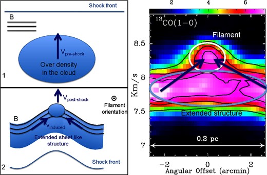
Left: Schematic view of the filament formation process due to compression of an overdensity by a shock wave (adapted from Inoue et al. 2018). The ambient B-field (indicated by the black lines) is parallel to the shock front. Right: Blow-up of the PV diagram (see figure 8) in 13CO(1–0) towards the filament YF for velocities between 6.8 km s−1 and 9 km s−1. The filament and the parent extended sheet-like structure are indicated with a white circle and a gray ellipse, respectively. The velocity gradients induced by the bending of the magnetic field are shown as converging arrows towards the filament (cf. subsection 4.2). (Color online)
4.2 Detection of an early stage of filament formation
The PV diagrams derived from C18O(1–0) and 13CO(1–0) observations perpendicular to the young filament YF (figure 8) show the filament detected at velocities around 8.2 km s−1, while a more extended structure is identified at velocities around 7.8 km s−1. The presence of a velocity gradient of about 0.5 km s−1 between YF and the extended structure suggests matter flow onto the young filament, which evolves, increasing in mass and density. This observed velocity pattern is in agreement with the formation of filamentary structures by accumulation of matter along magnetic-field (B-field) lines bent by a shock compression as proposed by Inoue et al. (2018) (see also Inoue & Fukui 2013; Vaidya et al. 2013). Appendix 3 presents a PV diagram perpendicular to the main axis of one of the filaments derived from the three-dimensional data cubes of the simulation by Inoue et al. (2018). The schematic view of the filament formation scenario is presented in figure 12 and can be described as the following:
The initial condition corresponds to an overdensity, a clump denser than its surrounding, present in the molecular cloud, formed, e.g., due to interstellar turbulence. The clump is threaded with an ordered magnetic field. This structure is about to interact with an interstellar shock front parallel to the magnetic field orientation and propagating towards it.
The interaction between the overdensity and the propagating shock front compresses the overdense structure into a sheet-like flattened structure. Due to the finite size of the initial overdense structure with respect to the shock front, this latter induces a bend both in the compressed sheet-like structure and in the frozen magnetic field structure. The shock front deformation along with the bending of the B-field lines increases the velocity component along the bent B-field lines, inducing a matter flow along the B-field lines and towards the maximum curvature, where matter converges as an elongated young filament (see subsection 3.1 of Inoue et al. 2018 for a more detailed explanation of this mechanism). Note that in a hydrodynamic oblique shock case, velocity gradients are also induced along the oblique shock front; however, the presence of an ordered and strong magnetic field is required to create a long and coherent filament.
Thanks to the ordered magnetic field structure, and the induced velocity gradients along the B-field lines, the filament is formed perpendicular to the ambient B-field lines. The filament is thus expected to be straight and uniform along its crest. The central density and total mass of the filament increase in time during the evolution of the sheet–filament system (as suggested by the numerical simulations of Inoue et al. 2018).
Our observations suggest that matter converges along the B-field lines with a rate of ρ vinf 2πR ≈ 48 |$M_{\odot } \, \rm pc^{-1}$| Myr−1 for ρ = 3 × 103 cm−3 estimated from |$N_{\rm H_{2}}=8\times 10^{20}{\rm \, cm^{-2}}$| and a size of 0.08 pc (see table 2), vinf = 0.5 km s−1, and R = 0.1 pc (see the right panel of figure 12). At this estimated rate, the forming filament increases in mass per unit length and may become critical (|$M_{\rm line,crit} \sim 16\, M_{\odot }\, \rm pc^{-1}$|) in ∼0.3 Myr. If there is sufficient gas mass in the parent sheet, the initially thermally subcritical young filament may increase in mass per unit length until it reaches a mass per unit length equal to the critical mass per unit length, becomes gravitationally unstable, and undergoes gravitational fragmentation into prestellar cores. On the other hand, when the filament cannot accumulate enough mass to become gravitationally bound, it may disperse, or be more vulnerable to expected forthcoming collisions/interactions with the surrounding environment.
Above we compared the expected velocity pattern from this scenario with the observation of the velocity field towards and around the filament YF. This comparison suggests that YF may be a young filament being formed by the convergence of matter along the B-field lines due to a flow induced by a shock compression. The scenario proposed by Inoue et al. (2018) is based on the main role of the relatively strong magnetic field. The only available data tracing the magnetic field towards this region are the Planck dust polarization maps at 350 GHz at a nominal resolution of 5′ (or 0.2 pc at the distance of 140 pc of the Taurus cloud; see, e.g., Planck Collaboration 2016b). The mean B-field orientation towards YF (averaged within 20′ × 20′) is ∼(112 ± 10)°, making an angle of ∼30° with respect to the orientation of YF on the plane of the sky. It is, however, difficult to draw conclusions about the relative orientation in three dimensions between the filament and the local B-field with the Planck data, because of (1) the low spatial resolution and the integration of the emission from several structures along the LOS, and (2) the projection effect, which may not give the true three-dimensional relative orientation between the B-field and the filament. From Planck dust polarization data we can only derive the plane-of-the-sky (POS) component of the line-of-sight average B-field.
Our results suggesting that the B-field structure towards YF, a presently subcritical, low-column-density filament, being perpendicular to the axis of YF, may be in contradiction with the orientation of the B-field lines derived from Planck dust polarization, supporting previous results derived from dust polarization observations as well as near-infrared and optical polarization observations (Planck Collaboration 2016a; Soler et al. 2016) where subcritical filaments are observed parallel to the B-field lines projected on the POS. This discrepancy may be due to the rapid transition from the thermally subcritical to the thermally transcritical/supercritical regimes resulting from the fast (∼10 |$M_{\odot } \, \rm pc^{-1}$| in ∼0.2 Myr) accretion of surrounding matter. Such short timescales may be statistically difficult to observe. The observations presented in this paper grasp the YF filament at an early stage of evolution, e.g., in the thermally subcritical stage. We suggest that YF will evolve and become thermally supercritical in the future. Molecular line observations towards the low-column-density filament and the analysis of their velocity field combined with the B-field structure would help to improve our understanding of the early stages of filament formation.
5 Summary and conclusions
In this paper we have presented molecular line mapping observations with the Nobeyama 45 m telescope towards a 10′ × 20′ field in the Taurus molecular cloud. The analyses and results derived from the OTF maps in 12CO(1–0), 13CO(1–0), and C18O(1–0) can be summarized as follows:
The C18O(1–0) integrated emission traces the elongated structure of the ∼1 pc-long thermally transcritical filament MF with column densities |$N_{\rm H_{2}}\gtrsim 5 \times 10^{21}\, {\rm cm^{-2}}$| as derived from Herschel data. The 13CO and 12CO integrated intensity maps show more extended emission around MF with column densities |$N_{\rm H_{2}}\gtrsim 1 \times 10^{21}\, {\rm cm^{-2}}$|.
Using PV diagrams and velocity channel maps derived from the 12CO(1–0), 13CO(1–0), and C18O(1–0) emissions we identified five structures at the following velocity ranges: B[4–5.4] km s−1, F1[5.4–6.2] km s−1, R1[6.2–7.2] km s−1, R2[7.2–8.1] km s−1, and F2[8.1–8.7] km s−1. The structures emitting at the velocities of B, R1, and R2 are identified as extended sheet-like structures surrounding the filament MF. The F2 velocity range corresponds to a thermally subcritical filament (YF) detected in the 13CO channel map.
We compared the optically thick 12CO(1–0) spectra “on” and “off” MF. In the B velocity range, we identified a decrease of 12CO intensity “on” MF that may result from absorption, suggesting that the structure emitting at these velocities may be located, at least partly, behind MF with respect to the LOS. Similar analysis suggested that the structures emitting at velocity ranges of R1 and R2 may be located in front of MF with respect to the LOS. We use these analyses to describe the relative positions of the sheet-like structures surrounding the filament MF.
We detected a velocity gradient along the crest of MF with velocity oscillations of ∼0.2 km s−1 on average, increasing towards the north part of the filament. We compared the velocity and column density structures along the filament crest. In the south part, MF has (1) larger column densities, (2) velocities in between that of SB and SR1, and (3) small velocity fluctuations. These suggest that MF may be compressed on both sides by SB and SR1. In the northern part, the velocities observed towards the low-column-density sections of MF are compatible with that of the SB structure emitting at the B velocity range. We suggest that, in the northern section, SB is interacting with MF, dragging its low-column-density parts. The higher-column-density fragments resist the sweeping and are observed at the LOS velocity of MF before interaction with SB.
The PV diagrams of 13CO and C18O towards YF show an elongated structure at velocities that differ by ∼0.5 km s−1 with respect to the velocity of YF. We compare the observed velocity structure with that expected from the filament formation model presented in Inoue et al. (2018); see also appendix 3. We suggest that our observations are compatible with the formation of a filament from the accumulation of matter along magnetic field lines induced by a shock compression due to a propagating wave. The observations suggest that a YF-like filament may form at a mass accretion rate of ∼50 |$M_{\odot } \, \rm pc^{-1}$| Myr−1 and become thermally critical in ∼0.2 Myr.
The propagation of interstellar shock waves, creating sheet-like molecular gas structures, may play an important role in the formation of filamentary structure in molecular clouds. These filaments increase in mass per unit length, accreting matter from the surrounding sheet until reaching the critical mass per unit length and becoming gravitationally unstable, fragmenting into star-forming cores. The same propagating shock waves may interact with already formed filaments resulting in the compression of additional matter onto the filaments or the removal/disruption of low-column-density parts. We suggest that such interactions may play an important role in the lifetime of filaments and their star formation activity.
Acknowledgements
We thank Kazuki Tokuda for discussions about the CO(2–1) observations of the Taurus molecular cloud. DA acknowledges an International Research Fellowship from the Japan Society for the Promotion of Science (JSPS). The 45 m radio telescope is operated by Nobeyama Radio Observatory, a branch of the National Astronomical Observatory of Japan. The numerical computations were carried out on an XC30 system at the Center for Computational Astrophysics (CfCA) of the National Astronomical Observatory of Japan. This work is supported by Grants-in-Aid from the Ministry of Education, Culture, Sports, Science, and Technology (MEXT) of Japan (15K05039 and 16H02160).
Appendix 1. Column density structure derived from Herschel observations
We present here the properties of the two filaments discussed in this paper as derived from Herschel dust continuum observations. The column density map shown in figure 13 is derived as explained in Palmeirim et al. (2013) (see, e.g., Marsh et al. 2016).2 We convolve the column density map to the 28″ resolution, the same as that of the molecular line maps studied in this paper.
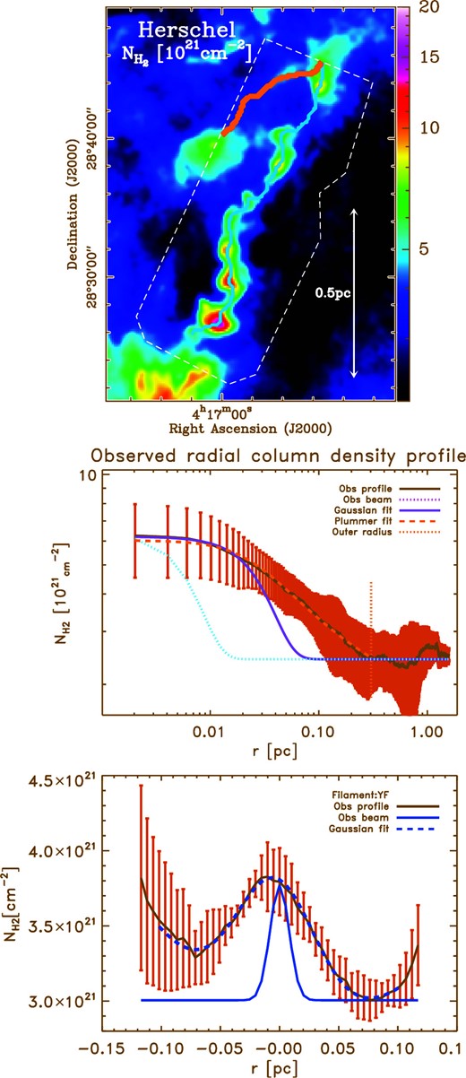
Top: Blow-up of the Herschel column density (|$N_{\rm H_{2}}$|) map (at the resolution of 28″) towards the region studied in this paper (same as figure 1). The blue and red skeletons show the crest of the filaments MF and YF traced with DisPerSE, respectively. The MF filament is traced on the column density map, while the YF filament has been traced on the 13CO(1–0) F2 channel map (right panel of figure 8). The white dashed contour shows the footprint of the CO maps observed with the Nobeyama 45 m telescope. Middle: Column density radial profile (in log–log) perpendicular to the main axis of MF and averaged along its crest. The blue and red curves show the best Gaussian and Plummer-like function fits, respectively. The vertical dotted red line marks the outer radius of the filament. The blue dotted curve shows the observational beam (HPBW = 28″). Bottom: Column density radial profile (in lin–lin) perpendicular to the main axis of YF. The best Gaussian fit and the observational beam are shown in dashed and solid blue curves, respectively. Table 2 summarizes the properties of MF and YF derived from Herschel observations. (Color online)
We trace the crest of the filaments using the DisPerSE algorithm Sousbie (2011). The MF filament is traced on the column density map, while the YF filament is traced on the 13CO(1–0) F2 channel map (right panel of figure 8). We derive radial column density profiles perpendicular to the filament crests and measure the filament properties as explained in Arzoumanian et al. (2011, 2018).
Figure 13 shows the column density map derived from Herschel observations and the radial column density profiles perpendicular to the MF and YF filaments and averaged along their crests. Table 2 summarizes the main properties of the filaments.
Appendix 2. Analysis of the observed spectra over the field
In this appendix we extend the analysis discussed in subsection 3.3, presenting averaged 12CO(1–0), 13CO(1–0), and C18O(1–0) spectra overlaid on the Herschel column density map (see figure 14). The spectra have been averaged over 2′ × 2′ squares and centered at different locations over the observed field on the filament MF as well as on its east and west sides. Figure 14 complements the spectra of figure 9, showing the variation of the spectra in the B velocity range suggesting possible absorption of the optically thick emission, while such features are not observed towards the R1 and R2 velocity ranges. We have used this analysis to suggest a three-dimensional structure of the observed portion of the cloud (see section 4).
![Herschel column density map at the resolution of 28″ (same as figure 1), overlaid with spectra averaged in 2′ × 2′ squares over the observed region. The velocity range is [4–10] km s−1, and the intensity range is from −1 to 18 K. The black, red, and blue spectra correspond to 12CO(1–0), 13CO(1–0), and C18O(1–0) emissions, respectively. The 13CO line is multiplied by a factor of 2 and the C18O line by a factor of 5. The shaded area on the plots for each spectrum show the same velocity ranges as the five channels discussed in the paper (see, e.g., figure 9). (Color online)](https://oup.silverchair-cdn.com/oup/backfile/Content_public/Journal/pasj/70/5/10.1093_pasj_psy095/3/m_pasj_70_5_96_f6.jpeg?Expires=1749203342&Signature=Bm5PuJ9nXKDM2oc~XpFtkExLRwC1NvyhWMABH0Fo4ScpnSVvq4Nj0tKFp2sT5r8VtFASv0d8ee~rwrN8LNsq921ktoelIZ8nfZiWMrCQoNBMI-kzOAoa3YlJAXOqzO9Iv8RIPSG2UYUBotgaLyXk2QipDMWPXC7e2XgPRgT5EKsSFMUWJQyoQb7-1kqBMymvYnUdwtA1kYnERJN8XHsM5wTA1brRua6-g~SvGpW~vhP01SB0MR9geDqKf2qqETSZTm5c5L6438E-yWwHcvsvogWS00MlRtOamytyFOc6lJpN1m3aTqfWPtL90YhKGsy3BAIU7SoL4ud21JNLve6mMQ__&Key-Pair-Id=APKAIE5G5CRDK6RD3PGA)
Herschel column density map at the resolution of 28″ (same as figure 1), overlaid with spectra averaged in 2′ × 2′ squares over the observed region. The velocity range is [4–10] km s−1, and the intensity range is from −1 to 18 K. The black, red, and blue spectra correspond to 12CO(1–0), 13CO(1–0), and C18O(1–0) emissions, respectively. The 13CO line is multiplied by a factor of 2 and the C18O line by a factor of 5. The shaded area on the plots for each spectrum show the same velocity ranges as the five channels discussed in the paper (see, e.g., figure 9). (Color online)
Appendix 3. Position–velocity diagram derived from the numerical simulation of filament formation by Inoue et al. (2018)
In this section we present the column density map and the PV diagram towards a filament extracted from the numerical simulation of Inoue et al. (2018), which studied the formation and evolution of filamentary structures induced by shock propagation in a turbulent molecular cloud. The numerical simulation is an isothermal MHD simulation using an adaptive mesh refinement technique. The simulation has been particularly tuned to study the formation of massive filaments forming high-mass stars, thus the densities and the velocity of the shock propagation are extreme compared to a low-mass star-forming region such as the Taurus molecular cloud; however, here we confirm that the filament observed in the simulation is formed by the mechanism explained in subsection 4.2, and has a velocity structure similar to that of the filament YF (see the right-hand panel of figure 12).
Figure 15 shows the background-subtracted column density structure of a filament from the simulation of Inoue et al. (2018) identified to be formed by the mechanism explained in subsection 4.2. We have selected a snapshot of the data (at t = 0.29 Myr after the shock compression) before the filament evolves into supercritical and shows gravitational collapse (that happens at t = 0.44 Myr). The mass per unit length of the filament at this epoch is ∼15 M⊙ pc−2, which is larger than the filament YF, but we confirmed that this filament is growing in mass as illustrated in the bottom left panel of figure 12.
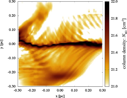
Background-subtracted column density structure of a filament from the simulation data by Inoue et al. (2018). (Color online)
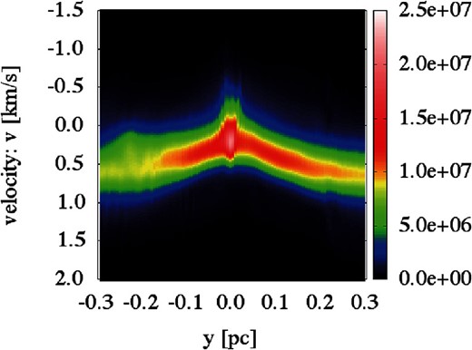
Position–velocity diagram perpendicular to the filament shown in figure 15 from the simulation by Inoue et al. (2018). This diagram is derived by averaging the simulated cubes along the filament length as described by equation (A1). The unit of the color scale of the map is given by equation (A1). (Color online)
Footnotes
See also the Herschel Gould Belt Survey Archive 〈http://gouldbelt-herschel.cea.fr/archives〉.
References
