


Abstract
The accretion-induced pulse period changes of the Be/X-ray binary pulsar X Persei were investigated over the period of 1996 January to 2017 September. This study utilized the monitoring data acquired with the RXTE All-Sky Monitor in 1.5–12 keV and the MAXI Gas-Slit Camera in 2–20 keV. The source intensity changed by a factor of 5–6 over this period. The pulsar was spinning down for 1996–2003, and has been spinning up since 2003, as already reported. The spin-up/down rate and the 3–12 keV flux, determined every 250 d, showed a clear negative correlation, which can be successfully explained by the accretion torque model proposed by Ghosh and Lamb (1979, ApJ, 234, 296). When the mass, radius, and distance of the neutron star were allowed to vary over a range of 1.0–2.4 solar masses, 9.5–15 km, and 0.77–0.85 kpc, respectively, the magnetic field strength of B = (4–25) × 1013 G gave the best fits to the observations. In contrast, the observed results cannot be explained by the values of B ∼ 1012 G previously suggested for X Persei, as long as the mass, radius, and distance are required to take reasonable values. Assuming a distance of 0.81 ± 0.04 kpc as indicated by optical astrometry, the mass of the neutron star is estimated as M = 2.03 ± 0.17 solar masses.
1 Introduction
The magnetic fields of binary X-ray pulsars have been directly measured utilizing cyclotron resonance scattering features (hereafter CRSF) in their X-ray spectra (e.g., Makishima 2016). The magnetic field strength B measured in this way is distributed in the range B/(1 + zg) = (1–7) × 1012 G (Yamamoto et al. 2014 and references therein), where zg ≃ 0.24 is the gravitational redshift at the neutron star (hereafter NS) surface. No accreting pulsars with B ≥ 1013 G have yet been discovered. However, this could be due to a selection effect, that the CRSF becomes difficult to detect at ≥100 keV (i.e, for B ≥ 1013 G) where the observational sensitivity becomes progressively lower. In order to search for such accreting NSs with higher magnetic fields, we need to invoke other methods such as pulse timing analysis or modeling of continuum spectra (Sasano 2015).
Using the MAXI Gas Slit Camera (GSC) data and some past measurements, Takagi et al. (2016) investigated long-term relations between the pulse period derivative |$\dot{P}$| and the fluxes of the binary X-ray pulsar 4U 1626−67. They adopted the accretion torque theory proposed by Ghosh and Lamb (1979), hereafter GL79, which describes |$\dot{P}$| as a function of the luminosity L, the pulse period P, the mass M, the radius R, and the surface magnetic field B of the NS. Then, employing B/(1 + zg) = 3.2 × 10¹² G measured with a CRSF (Orlandini et al. 1998), the GL79 model was confirmed to accurately explain the observed relation between |$\dot{P}$| and L of 4U 1626−67, including both the spin-up and spin-down phases. This means that accurate measurements of |$\dot{P}$| over a sufficiently wide range of L for a binary X-ray pulsar would conversely allow us to estimate its B.
X Persei (4U 0352 + 309) is a high-mass X-ray binary system, consisting of a Be-type star and a magnetized NS. Its pulse period of P ∼ 835 s, which is relatively longer than those of other pulsars, was independently discovered by Ariel 5 and Copernicus (White et al. 1976). The distance to the source is estimated as D = 0.81 ± 0.04 kpc by its optical parallax derived from the GAIA Astrometry.1 With X-ray observations, Delgado-Martí et al. (2001) determined the orbital period of X Persei as Porb = 250.3 ± 0.6 d, and derived an eccentricity of e ∼ 0.11, which is considerably smaller than those of typical Be/X-ray binaries, e ≥ 0.3.
X Persei was spinning up at a rate of |$\dot{P}\sim -1.5 \times 10^{-4}\:$|yr−1 until 1978, when it turned into a phase of spin down at a rate of |$\dot{P}\sim 1.3 \times 10^{-4}\:$|yr−1 (Delgado-Martí et al. 2001). In 2002 the pulsar returned to the spin-up phase, and has since been spinning up until today. This spin up/down alternation implies that the source is close to a torque equilibrium, and hence the long P suggests a strong magnetic field, because we then expect |$B\sim L^{\frac{1}{2}}P^{\frac{6}{7}}$| (Makishima 2016)
In the 2–20 keV range, the spectrum of X Persei can be fitted by a power-law model with an exponential cutoff (Di Salvo et al. 1998), which is typical of accreting X-ray pulsars. However, in the 20–100 keV band, the spectrum of X Persei is much flatter and harder than those of other X-ray pulsars, and lacks a steep cutoff (Sasano 2015). Sasano (2015) empirically quantified this shape of the spectrum in comparison with those of other pulsars (mostly with B measured), and obtained an estimate of B ∼ 1013 G. Although Coburn et al. (2001) noticed a spectral dip at ∼29 keV in an RXTE/PCA spectrum, and regarded it as a CRSF corresponding to B/(1 + zg) = 2.5 × 10¹² G, the feature is too shallow and broad for that interpretation, and can be explained by a combination of two continuum components without a local feature (Doroshenko et al. 2012; Sasano 2015). Thus, the strong-field property of X Persei is also suggested by its spectral properties.
In the present paper, we report the long-term continuous observations of the fluxes and P of X Persei by RXTE and MAXI. Applying the GL79 model to the derived |$\dot{P}$|–L relation, we then estimate B and M for the NS in this binary.
2 Observation
2.1 MAXI/GSC
Since 2009 August, MAXI (Matsuoka et al. 2009) on board the International Space Station (ISS) has been continuously scanning the X-ray sky every 92 min of the ISS orbital period. We derived the data for X Persei from the MAXI/GSC (Mihara et al. 2011; Sugizaki et al. 2011) using the On-Demand System2 provided by the MAXI team. This data analysis scheme enables us to extract images, light curves, and energy spectra of a given source by specifying its coordinates and observation times. The on-source events and background events, both in 2–20 keV, were derived using standard regions. Every 92 min we thus obtained a background-subtracted data set (an energy spectrum) with an integration time of ∼60 s corresponding to a single scan transit of the source. Since this is considerably shorter than the pulse period of X Persei (∼835 s), the data obtained with a single scan are just a snapshot at a certain pulse phase. These data sets have been combined into a 2–20 keV light curve from MJD 55054 to MJD 58049 and 12 energy spectra each summed over the 250 d orbital period. The 250 d averaged spectra have statistics high enough to yield accurate fluxes.
2.2 RXTE/ASM
The All-Sky Monitor (ASM: Levine et al. 1996) on board the RXTE satellite (Bradt et al. 1993) continuously monitored the whole X-ray sky from MJD 50087 to MJD 55927. For this entire period, we retrieved the RXTE/ASM dwell-time light curves of X Persei in four energy ranges, namely 1.5–12.0 keV, 1.5–3.0 keV, 3.0–5.0 keV, and 5.0–12.0 keV.3 These light curves were used to obtain P and the fluxes.
2.3 RXTE/PCA
In order to cross check the validity of the fluxes of RXTE/ASM and MAXI/GSC, RXTE/PCA data were also used. Since the PCA data are generally too short and sparse for the accurate determination of P and calculation of |$\dot{P}$|, these data were not used for pulse period analysis. Throughout the 16-year RXTE mission, a total of 156 pointing observations were performed on this source by the Proportional Counter Array (PCA: Jahoda et al. 2006). Those PCA observations were made in the period from MJD 50161 to MJD 52687. In this duration, one of the PCA units, PCU 2, had longer exposure times than the others. Thus, we have used the data taken by PCU 2 only. An inspection of the operational status of PCU 2 indicated that some of the data sets were acquired under bad conditions (e.g., large offset angles). We discarded those data sets, and utilized 136 pointing observations (total exposure time of 640 ks) to extract the spectra.
2.4 Long-term light curves
To investigate intensity variations of X Persei we have binned all the RXTE/ASM and MAXI/GSC data into 25 d-bin light curves. The derived long-term light curves from 1996 to 2017 are shown in figure 1, where the background-subtracted count rate is normalized to that of the Crab Nebula. Thus, X Persei showed moderate X-ray intensity variations up to a factor of 5–6. The intensity is not apparently modulated at the orbital period, presumably because of the small eccentricity. Instead, in 2003, 2010, and 2017 the intensity increased to 50 mCrab and dropped to 25 mCrab in one orbital period, suggesting a 7 yr super-orbital periodicity.
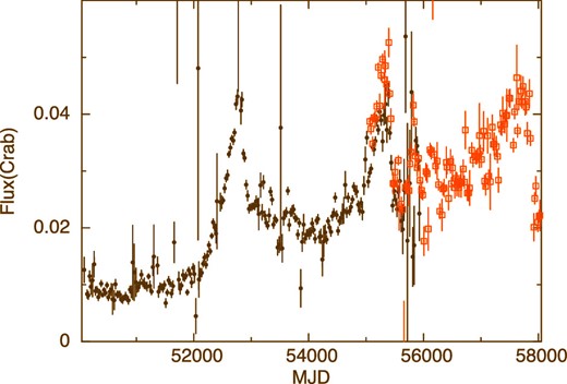
Long-term (1996–2017) light curves of X Persei in 25 d bins, expressed in Crab units. The filled circles and open squares are data from the RXTE/ASM (1.5–12 keV) and the MAXI/GSC (2–20 keV), respectively. (Color online)
3 Analysis and results
In order to calculate |$\dot{P}$|, it is necessary to first determine P accurately, with a reasonably dense sampling. For this purpose, the times of individual light-curve bins were converted to those to be measured at the solar center; this heliocentric correction, instead of the more complex barycentric correction, is sufficient for the present purpose because of the long pulse period. Then, we performed time corrections for the binary orbital motion of X Persei, assuming the circular orbit parameters Porb = 249.9 d, an epoch of 90° mean orbital longitude of Tπ/2 = 51215.5 (MJD), and a semi-major axis of ax sin i = 454 lt-s, from table 2 of Delgado-Martí et al. (2001). The small eccentricity (e ∼ 0.11) affects the value of P at most by ±0.010 s in a 70 d analysis (subsection 3.1) and ±0.001 s in a 250 d analysis (subsection 3.2); these are smaller than the typical errors of the P measurements.
3.1 Refinement of the orbital period
As a preliminary attempt to confirm the arrival-time corrections, we determined the pulse period every 70 d for MJD 55450–57020, when the luminosity stayed relatively constant. The epoch-folding method described in subsection 3.2 was employed, assuming |$\dot{P}=-7\times 10^{-9}\:$|s s−1, which is the average value of |$\dot{P}$| during this time period. The result is shown with black points in figure 2. Although the values of P confirm the spin-up trend in general, the data points show a wiggling behavior around the trend, with a typical period of four data points, or ∼280 d. Since the flux in figure 1 is not modulated at this period, the effect is unlikely to be caused by accretion-torque changes. Instead, it could be due to slight discordance of the orbital phase, which in turn arose from an accumulation of the error of Porb for 12–16 yr since the observation by Delgado-Martí et al. (2001). We searched for a better orbital period as follows, assuming that T0 = 51215.5 (MJD) and ax sin i = 454 lt-s are correct. First, we repeated this analysis by changing the trial value of Porb from 249.9 d to 251.8 d with a step of 0.3 d or finer. Then, from the pulse-period history obtained in this way, we subtracted a trend line represented by |$\dot{P}=-7\times 10^{-9}\:$|s s−1. Finally, the residual pulse period was folded at the employed Porb. The black points in figure 2 show the folded residuals assuming, for example, Porb = 249.9 d, where large residuals make a constant-line fit unacceptable with χ2 = 134 (for d.o.f. = 3). The values of χ2 derived from this Porb scan are plotted in figure 3, and the orbital profile of the residuals for four representative cases (including the one with Porb = 249.9 d) are presented in figure 2. Requiring that the residual pulse-period modulation at the assumed Porb should be minimized, the best orbital period was estimated as |$P_{\rm orb}=251.0^{+0.2}_{-0.1}$| d (1 σ error), which is still not away from the 2 σ error range given by Delgado-Martí et al. (2001). We hereafter use this value for the binary orbital motion corrections.
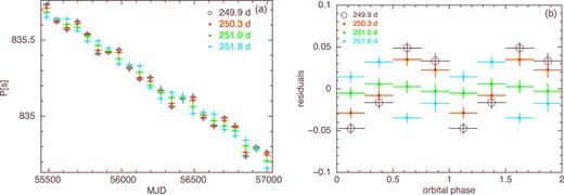
(a) Pulse periods of X Persei determined every 70 d with the MAXI/GSC. The colors specify different values of Porb employed to correct the pulse arrival times for the orbital motion of the NS. (b) Pulse-period residuals, obtained from panel (a) by subtracting a linear trend and folding at the assumed Porb.
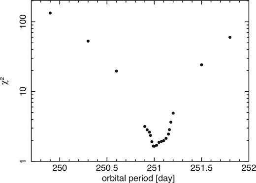
Values of χ2 from a constant fit to the residual profiles such as shown in figure 2, presented as a function of the assumed Porb.
3.2 Pulse timing analysis
3.2.1 Measurements of P
With a successfully updated Porb, we employed the best orbital period in the correction of the binary motion. Then, we analyzed the entire RXTE/ASM and MAXI/GSC data of X Persei with the standard epoch-folding method (Leahy et al. 1983) to determine P for X Persei every 250 d. This time period, which is longer than employed in subsection 3.1 and is close to Porb, was chosen to accurately estimate |$\dot{P}$|, which is important in the GL79 formula. The employed energy band was 1.5–12 keV for the RXTE/ASM and 2–20 keV for MAXI/GSC. The number of bins of the folded pulse profile was chosen as 16, because one MAXI data point is an accumulation over about 60 s. We assumed a constant but free |$\dot{P}$| during each 250 d time period, and searched for a pair (P, |$\dot{P}$|) that maximized the χ2 of the folded 16-bin pulse profile against the constant-intensity hypothesis.
An example of a χ2 map on (P, |$\dot{P}$|) is shown in figure 4a, and the corresponding folded pulse profile using (P, |$\dot{P}$|) at the maximum χ2 is shown in figure 4b. The pulse profile has a sinusoidal shape, not only in this particular case, but also in other intervals.

(a) Color map of the 2–20 keV pulse significance in terms of χ2, for MJD 56300–56549, shown on the P–|$\dot{P}$| plane. The best-fit values are P = 835.090 ± 0.002 s and |$\dot{P}=-(6.3\pm 0.7)\times 10^{-9}\:$|s s−1. (b) Background-subtracted 2–20 keV pulse profile of X Persei in MJD 56300–56549, folded with the χ2-maximum parameters.
The derived values of P are shown in figure 5b, together with the 250 d-averaged 3–12 keV flux to be described in the next section. The 1 σ errors of P were estimated with the Monte Carlo method of Leahy (1987). As Lutovinov, Tsygankov, and Chernyakova (2012) and Acuner et al. (2014) reported, the pulsar changed from a spin-down phase to a spin-up phase around MJD 52000, when the X-ray flux started increasing. Since then, X Persei has been in the spin-up phase at least until MJD 58049.
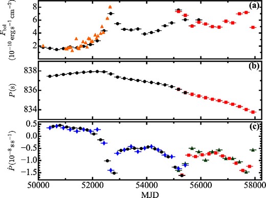
(a) 3–12 keV fluxes of X Persei obtained with the RXTE/ASM (black circles), the MAXI/GSC (red squares), and the RXTE/PCA (yellow triangles). The MAXI/GSC fluxes have been converted as described in the text. (b) Intrinsic pulse period of X Persei, after the heliocentric and binary orbit corrections. In both panel (a) and panel (b), one data point covers a 250 d time interval. (c) Comparison between |$\dot{P}_{\chi ^2}$| (blue diamonds and green triangles) and |$\dot{P}_{\rm diff}$| (black and red).
3.2.2 Calculations of |$\dot{P}$|
Although |$\dot{P}$| was thus estimated every 250 d, the calculation of |$\dot{P}$| can also be done by taking the difference between two adjacent points of P. Let us denote |$\dot{P}$| from the P–|$\dot{P}$| plane (e.g., figure 4) as |$\dot{P}_{\chi ^2}$|, and |$\dot{P}$| from the difference between adjacent P measurements as |$\dot{P}_{\rm diff}$|. Then, as shown in figure 5c, |$\dot{P}_{\rm diff}$| is consistent with |$\dot{P}_{\chi ^2}$|, and has smaller uncertainty. Therefore we employ |$\dot{P}_{\rm diff}$| hereafter.
3.3 Calculation of the energy flux
The energy flux of X Persei at individual epochs can be derived from the MAXI/GSC and the RXTE/ASM data. In addition, a limited amount of data from the RXTE/PCA were utilized. In order to minimize the systematic differences among the three instruments, we decided to use their common energy band, 3–12 keV. Below, we describe how the fluxes were derived with the three instruments.
3.3.1 The MAXI/GSC data
The 2–20 keV energy spectra of X Persei with the MAXI/GSC were accumulated over the same 250 d time periods as in subsection 3.2, and fitted individually by a power law with an exponential cutoff. The interstellar absorption was fixed to NH = 3.4 × 1021 cm−2, derived from an XMM-Newton observation (La Palombara & Mereghetti 2007), because it cannot be determined independently with the MAXI/GSC. The spectral fits were acceptable in all the time periods, with a reduced chi-square of |$\chi _{\rm \nu }^2 \sim 1$|. We then calculated the unabsorbed 3–12 keV fluxes from the best-fit models. For example, the best-fit model for MJD 56300–56549 has a photon index of Γ = 0.67 ± 0.13, a cutoff energy of |$5.57\pm 0.76\, \rm keV$|, and a normalization of (8.4 ± 0.7) × 10−2 with χ2 = 119 for 105 d.o.f.
By analyzing all the MAXI/GSC spectrum in the same way, the 2–20 keV fluxes were obtained as (9–14) × 10−10 erg cm−2 s−1, and those in 3–12 keV as (6–10) × 10−10 erg cm−2 s−1. The latter results are presented with red squares in figure 5a, in comparison with the |$\dot{P}$| determinations made in subsection 3.3. (A correction factor of 0.78 was multiplied in order to match the data to the RXTE/ASM data. See sub-subsection 3.4.2.) In figure 5a, we can reconfirm the intensity variations seen in figure 1.
3.3.2 The RXTE/ASM data
By adding the dwell-time light curves in 3–5 keV and 5–12 keV, the 3–12 keV count rates averaged over the individual 250 d time periods were obtained. We converted the 3–12 keV count rates into 3–12 keV fluxes using the WebPIMMS system.4 Since this conversion requires knowledge of the spectrum shape of the source, we followed the results of the MAXI spectroscopy and assumed a power-law spectrum with Γ = 1.7 and NH = 3.4 × 1021 cm−2 (La Palombara & Mereghetti 2007) in all the 250 d time periods. Although the MAXI spectra cover only the spin-up phase after 2009, our assumption on the spectral shape is justified by Lutovinov, Tsygankov, and Chernyakova (2012), who analyzed the 2–20 keV RXTE/PCA data of X Persei in both the spin-down and spin-up phases, and found no significant difference in the spectral shape.
The unabsorbed fluxes thus estimated with the RXTE/ASM data are shown in figure 5a by black filled circles. Over the time range when the MAXI and RXTE/ASM results overlap, we found that the MAXI fluxes were systematically higher, by ∼25%, than those of the RXTE/ASM. Since the RXTE/ASM fluxes are consistent with BeppoSAX observations (Di Salvo et al. 1998) and the RXTE/PCA measurements described in the next section, the MAXI/GSC fluxes have been corrected to match the RXTE/ASM measurements by multiplying by a factor 0.78. The investigation of this difference is beyond the scope of this work.
3.3.3 The RXTE/PCA data
First, we investigated the individual spectra obtained by the 136 pointing observations. Although some of them have short exposure times (≤1 ks), these data were confirmed to have sufficient quality to analyze the 3–12 keV X-ray spectra. The PCU2 spectra were fitted by a power-law model with an exponential cutoff, incorporating a low-energy absorption factor with NH = 3.4 × 1021 cm−2 (again, fixed). The model successfully described all the PCU2 spectra. Next, we calculated unabsorbed 3–12 keV fluxes of all these observations, and averaged them typically every ∼50 d. The results are shown in figure 5a with yellow triangles. Thus, the PCA and ASM results are consistent with each other, justifying the correction of the MAXI/GSC fluxes. As already noted in subsection 2.3, we did not utilize the PCA data in the pulse-timing studies.
3.3.4 Estimation of the bolometric flux
Since the luminosity used in the GL79 formalism is the bolometric value Lbol, we converted the 3–12 keV fluxes to the bolometric ones, Fbol. For this purpose we employed the best-fit model to the 0.1–200 keV spectrum obtained with BeppoSAX in 1996 September (spin-down phase), and that in the 1–100 keV band obtained with Suzaku in 2012 September (spin-up phase), derived by Di Salvo et al. (1998) and Sasano (2015), respectively. The conversion factor from the 3–12 keV to 0.1–200 keV fluxes was calculated as 2.605 in BeppoSAX and 2.611 in Suzaku, respectively. Since the two factors agree very well within ≤0.1%, in agreement with Lutovinov, Tsygankov, and Chernyakova (2012), we used a factor of 2.61 for both the spin-down and spin-up phases, and multiplied it to all the data points in figure 5a.
3.3.5 The correlation between |$\dot{P}$| and Fbol
The derived |$\dot{P}$| and Fbol values of X Persei, spanning 22 yr, are shown in figure 6. Thus, we find a clear negative correlation between |$\dot{P}$| and Fbol for X Persei. Although a few data points are outlying, |$\dot{P}$| basically behaves as a single-valued function of Fbol as the latter varies by a factor of ∼5. After renormalizing the MAXI/GSC fluxes (sub-subsection 3.3.2), the data points from the two instruments are generally consistent with one another. Furthermore, a single correlation appears to persist through the spin-up and spin-down phases, without exhibiting any drastic changes toward lower fluxes. Therefore, the system is considered to still be free from the so-called propeller effect, which might set in at very low accretion rates. Thus, the overall source behavior in figure 6 is very similar to the case of 4U 1626−67 studied by Takagi et al. (2016), wherein the GL79 model was given a very successful explanation.
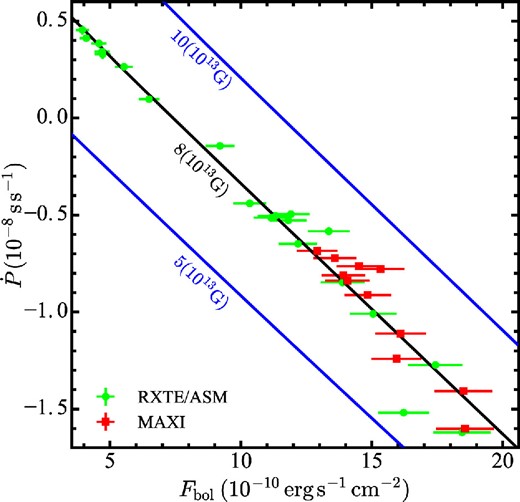
|$\dot{P}$| and Fbol measurements with the RXTE/ASM (circles) and MAXI/GSC (squares), compared with the GL79 predictions. The middle line shows the best-fit GL79 relation. It can be represented by multiple sets of parameters (figure 9), including a particular case of M = 2.05 M⊙, R = 12.9 km, D = 0.81 kpc, and B = 8 × 10¹³ G. The top and bottom lines show predictions when B is changed, with the other parameters kept unchanged. (Color online)
4 Application of the GL79 model
4.1 Comparison between the observational results and GL79
The final step of our analysis is to fit the |$\dot{P}$|–Fbol relation in figure 6 with the GL79 model, to constrain the parameters of the NS in X Persei: M, R, and B. We use the same procedure as described in Appendix 1 of Takagi et al. (2016), as briefly reviewed below.
By substituting equations (2) through (7) into equation (1), we can calculate a theoretical |$\dot{P}$| vs. L37 relation to fit the observed data points in figure 6. However, the prediction is subject to uncertainties in the parameters involved, namely M, R, D, and B. Because B is the least constrained of these, and is our prime interest, we restricted the ranges of M, R, and D to 1.0–2.4 M⊙, 9.5–15 km, (e.g., Özel & Freire 2016; Bauswein et al. 2017) and 0.81 ± 0.04 kpc (section 1), respectively, and aimed to estimate B. Since the correlation is almost linear, which has two free parameters, we specified trial values of (B, D), and optimized (M, R) to minimize the χ2.
An example of the best-fit GL79 prediction is shown with a black line in figure 6, where B = 8 × 10¹³ G was assumed and the best-fit parameters were obtained as (M, R, D) = (2.05 M⊙, 12.9 km, 0.81 kpc). By introducing a 5.9% systematic error to Fbol, the data points were explained successfully (χ2 = 29, d.o.f. = 29), including both the spin-up and spin-down phases, since n(ωs) can take both positive and negative values. However, due to the heavy model degeneracy, the parameters cannot be constrained uniquely. Instead, the same best-fit solution in figure 6 can be reproduced by multiple sets of (M, R, D, B). For example, the sets (2.02 M⊙, 14.1 km, 0.81 kpc, 6 × 10¹³ G) and (2.05 M⊙, 9.5 km, 0.81 kpc, 23 × 1013 G) give essentially the same prediction, and hence the same χ2.
The black circles of figure 7 represent the minimum χ2 values as a function of the assumed B, where M, R, and D are allowed to move freely within their respective constraints. We thus find that the same best-fit solution is obtained over a range of B = (5–23) × 1013 G. Below B = 5 × 10¹³ G, the fit χ2 starts increasing because R is saturated at R = 15 km. In the same way, the fit worsens above B = 23 × 1013 G due to R fitting the assumed floor at R = 9.5 km. This is mainly because the value of |$\mu \sim \frac{1}{2} {BR^3}$| is roughly fixed by the zero-crossing point in figure 6, that is, the spin up/down boundary (Takagi et al. 2016). The effect of changing B, with the other parameters kept fixed, is shown by the top and bottom lines in figure 6. Under this constraint, only the zero-crossing point moves, with the slope almost unchanged, and the data favors B = 8 × 10¹³ G.
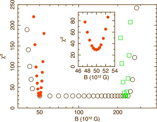
χ2 value of the fit to figure 6 with equation (1), shown as a function of the assumed B. The open circles show the results when M, R, and D are allowed to take free values within the allowed ranges. The filled circles exemplify the case with M = 1.90 M⊙, R = 14.6 km, and D = 0.77 kpc, whereas the open squares assume M = 2.05 M⊙, R = 9.5 km, and D = 0.81 kpc. The inset shows the detail at B = (46–54) × 1012 G. (Color Online)
The filled circles and open squares in figure 7 represent the behavior of χ2 when the set of (M, R, D) are fixed to the best values at B = 5 × 10¹³ G and those for B = 23 × 1013 G, respectively. When M and D are fixed, the increase of χ2 thus becomes steeper than the case when they are free. In short, the present study indicates B = (5–23) × 1013 G even allowing M, R, and D to vary freely over the assumed uncertainty ranges.
As represented by equation (9) in Takagi et al. (2016), the slope of the GL79 relation depends mainly on M and D. Since |$\dot{P}$| is proportional to I−1, and hence to M−1, the slope flattens as M increases. Figure 8 presents the same data set as figure 6, but is meant to show how the GL79 prediction depends on M. Thus, the data prefer a relatively high value of M.
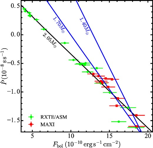
The data points and the best-fit line are the same as in figure 6. The other two lines are for M = 1.70 M⊙ and M = 1.40 M⊙ with the same R, D, and B as in the black line. (Color online)
So far, we have confirmed the argument by Takagi et al. (2016) that figure 6 can constrain, with its zero-crossing point and the data slope, two out of the four model parameters (M, R, D, and B). In other words, specifying two of them can allow us to estimate the remaining two through the GL79 fit to figure 6. Choosing D and B as the two input parameters, figure 9 shows how M and R are determined. The dashed lines in figure 9 represent grids of constant D and B. Thanks to the accurate distance determination, M is relatively well constrained, although we need to consider the systematic errors involved in equation (1). In these arguments using figure 9, we have assumed that the radius is in the range of R = 9.5–15 km, based on a recent equation of state of NSs (Özel & Freire 2016) and the GW170817 observations (Bauswein et al. 2017).
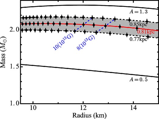
Sets of (M, R) accepted by the present data. The constant-B and constant-D grids are represented by dashed lines. In particular, the M–R relation fixing D = 0.81 kpc is represented by the middle solid line. The bottom and top solid lines are those when the normalization of equation (1) is chosen as A = 0.5 or A = 1.3, both with D = 0.81 kpc. (Color online)
4.2 Systematic model uncertainties
In the previous section, we considered how the data can constrain M, R, D, and B, when the first three of them are allowed to move freely over their predefined uncertainty ranges, whereas B can take any positive value. However, we have yet to consider another source of systematic error, namely the uncertainty in the GL79 model itself. This may be expressed by multiplying the right-hand side of equation (1) by a normalization factor A, and allowing it to take values other than unity.
Along the above line of argument, Takagi et al. (2016) showed that the MAXI/GSC data of the low-mass X-ray pulsar 4U 1626−67 can be explained very well with A ≈ 1.0. Analyzing the MAXI/GSC and Fermi/GBM data of 12 Be pulsars in a similar manner, Sugizaki et al. (2017) argued that the values of A also have a mean around unity, but scatter from ∼0.3 to ∼3 among the 12 sample objects. Furthermore, Sugizaki et al. (2017) successfully decomposed this scatter into the following three major sources: One comes from the model assumption that the emission of a pulsar is completely isotropic, which is obviously not warranted because X Persei shows strong pulsations. As adopted by Sugizaki et al. (2017), this uncertainty may amount to a factor of 2, after Basko and Sunyaev (1975). Another uncertainty lies in the angle between the magnetic axis and the accretion plane; it can affect the dipole magnetic field strength at large distances by another factor of 2 (Wang 1997). The last uncertainty is that in the distance.
In the present case, the last uncertainty, namely that in D, can be ignored, because it is rather small, and was already considered before introducing A. Therefore, we may presume that A takes a value from 0.5 to 1.9. Then, the model fitting was repeated by multiplying A into the right-hand side of equation (1), and changing it from 0.5 to 1.9. For example, two lines with A = 0.5 and A = 1.3 are shown in figure 9, where D = 0.81 kpc is fixed. As a result, the mass and magnetic field ranges have somewhat increased to M = 1.3–2.4 M⊙ and B = (4–25) × 1013 G, respectively.
5 Discussion and conclusion
Using the RXTE/ASM and MAXI/GSC data, together spanning 22 yr, we studied the spin-period change rate |$\dot{P}$| and the bolometric luminosity L of X Persei. |$\dot{P}$| was confirmed to behave as a single-valued and approximately linear function of L (figure 6), covering both the spin-down (|$\dot{P}>$| 0) phase before MJD 52200 and the spin-up (|$\dot{P}<0$|) phase afterwards. At the present spin period of P ∼ 837 s, the torque equilibrium condition (|$\dot{P}=0$|; the zero-crossing point in figure 6) is realized at L = 5 × 1034 erg s−1 assuming D = 0.81 kpc. In addition, the orbital period of X Persei has been updated to |$251.0^{+0.2}_{-0.1}$| d.
5.1 The magnetic field of the neutron star in X Persei
By fitting the observed |$\dot{P}$| vs. L relation with the theoretical GL79 model, incorporating its observational calibrations (Takagi et al. 2016; Sugizaki et al. 2017), we have estimated the surface dipole magnetic field of X Persei as B = (4–25) × 1013 G. Since the equilibrium values of L and P together specify the magnetic dipole moment (∝BR3) rather than B itself, the derived estimate of B is most strongly affected by the uncertainty in R. In fact, as in figure 7, the lower and upper limits of the derived B respectively correspond to the upper bound of R = 15 km and the lower bound of R = 9.5 km, which we assumed as conservative limits. If R is further restricted in future studies, e.g., by gravitational wave observations, the range of B will become narrower accordingly. Regardless, the present results show that X Persei has a significantly stronger magnetic field than ordinary accretion-powered pulsars (B ∼ 1012 G).
Our result is consistent with the suggestions from spectral studies by Doroshenko et al. (2012) and Sasano (2015). These authors noticed that the spectrum of X Persei, extending to 160 keV (Lutovinov et al. 2012) without a clear cutoff, is qualitatively distinct from those of ordinary X-ray pulsars, which decline steeply above 20–30 keV at least partially due to the presence of CRSFs (Makishima 2016). Because the spectral cutoff of X Persei must appear at rather high energies, its CRSF, if any, would be present above ∼400 keV, corresponding to B ≳ 4 × 10¹³ G.
As mentioned in section 1, the spectrum of X Persei exhibits a shallow and broad dip at ∼30 keV (Coburn et al. 2001; Lutovinov et al. 2012). Coburn et al. (2001) interpreted it as a CRSF, and proposed a value of |$B\sim 10^{12}\, \rm G$|. However, Doroshenko et al. (2012) fitted the spectrum of X Persei successfully with two Comptonization models (to be interpreted as thermal and bulk Comptonization), without invoking a CRSF structure. A very similar result was obtained by Sasano (2015) from a broad-band Suzaku spectrum of X Persei. Thus, the dip around 30 keV can be better interpreted as a “crossing point” of the two Comptonization components, rather than a CRSF.
5.2 Luminosity of X Persei
The GL79 relation which we employed, equation (1), assumes mass accretion from an accretion disk. This condition is probably satisfied in 4U 1626−67, and in the 12 Be pulsars studied by Sugizaki et al. (2017). Specifically, these Be binaries are considered to be accreting from the circumstellar envelopes of their Be-type primaries (e.g., Okazaki et al. 2013), through accretion disks that form near the pulsars. Compared to these typical Be X-ray binaries, X Persei has an unusually wide and nearly circular orbit with ax ∼ 2 au (Delgado-Martí et al. 2001), together with a very low luminosity that lacks orbital modulation. In spite of these peculiarities, we believe that X Persei is also fed with an accretion disk rather than via stellar-wind capture, for the following three reasons.
The first reason supporting the disk-accretion scheme is that the primary star of X Persei, of spectral type (O9.5III-B0V)e (Lyubimkov et al. 1997), is not expected to launch massive stellar winds. Its luminosity of ∼3 × 10⁴ L⊙ and the empirical stellar wind intensity (Cox 2000) predict a wind mass-loss rate of ≲10−7.5 M⊙ yr−1. At a distance of 2 au (appropriate for the NS of X Persei) from the star, and assuming a typical wind velocity of 108 cm s−1, this would yield a wind-capture X-ray luminosity of ≲1032 erg s−1, which is much lower than the actually observed values of 1034–35 erg s−1. Second, the spectra of X Persei show neither strong iron-K emission lines (with an equivalent width of at most 7.5 eV; Maitra et al. 2017), nor variable high absorption. According to Makishima et al. (1990), these properties of X Persei support the scheme of mass accretion from the Be envelope, rather than from the stellar winds. Finally, the Be envelope is likely to be actually feeding the pulsar, because a positive correlation was observed between the optical Hα line intensity and the X-ray flux over 2009–2018 (Zamanov et al. 2018), involving the possible 7 yr periodicity, although no clear correlation was observed before 2009 (Smith & Roche 1999; Reig et al. 2016).
From the above arguments, X Persei is considered to have the same accretion scheme as the other Be X-ray binaries. Its unusually low luminosity, without orbital modulation, can be attributed to to its very wide and nearly circular orbit, along which the stellar envelope is expected to have a rather low density. Incidentally, the possible 7 yr X-ray periodicity (subsection 2.4), correlated with the Hα variations (Zamanov et al. 2018), may be produced by some long-term changes in the circumstellar envelope, as pointed out by Laplace et al. (2017).
5.3 Mass of the neutron star in X Persei
While the zero-crossing point of the L vs. |$\dot{P}$| correlation in figure 6 is most sensitive to the magnetic dipole moment of the pulsar, the slope of the correlation specifies mainly M (Takagi et al. 2016). Thus, assuming D = 0.81 ± 0.04 kpc, and neglecting the systematic model uncertainty (subsection 4.2), the NS in X Persei is constrained to have M = 2.03 ± 0.17 M⊙, as in figure 9. Therefore, the object is suggested to be somewhat more massive than typical NSs with M ∼ 1.4 M⊙.
As shown in figure 9, the systematic GL79 model uncertainty affects the estimate of M, and its inclusion widens the range to M = 1.3–2.4 M⊙. Then, the canonical value of M = 1.4 M⊙ can no longer be excluded. Nevertheless, in order for the object to have M = 1.4 M⊙, we need to invoke the smallest value of A ∼ 0.5. This would, in turn, require, for example, that the emission from X Persei is strongly beamed away from our line of sight, and we are underestimating its spherically averaged luminosity by a factor of 2. Thus, the data still favor a relatively high mass (e.g., ∼2 M⊙).
Let us tentatively assume that the NS in X Persei is indeed massive. Then, this must be from its birth, because the accretion rate of X Persei (∼1 × 10⁻¹² M⊙ yr−1) and its estimated lifetime (∼107 yr) mean a negligible mass increase due to accretion. We hence arrive at an interesting possibility, that a fraction of NSs could be born with a strong magnetic field (B ≥ 1013 G) together with a rather high mass. Such a native difference, if true, might in turn reflect different mechanisms of NS formation. Even excluding the case of accretion-induced collapse of white dwarfs, NSs in Be X-ray binaries may be produced via supernovae of either electron-capture type or gravitational core-collapse type. As discussed by Kitaura, Janka, and Hillebrandt (2006), the former types are likely to leave rather standard NSs with ∼1.4 M⊙ and B ∼ 1012 G, as is possibly the case with the Crab pulsar (Moriya et al. 2014). In contrast, core-collapse supernovae might sometimes yield NSs with a higher M and a stronger B, as represented by X Persei. Even in that case, it is an open question whether a higher mass necessarily leads to a stronger field, or these two quantities scatter independently.
Acknowledgements
The authors are grateful to all MAXI team members for scientific analysis. This work was supported by KAKENHI, Scientific Research (C), No. 18K03694.
Footnotes
References
