


Abstract
The ejecta kinematics of supernova remnants (SNRs) is one of the crucial clues to understanding the explosion mechanism of type Ia supernovae (SNe). In particular, the kinematic asymmetry of iron-peak elements provides the key to understanding the physical processes taking place in the core of the exploding white dwarfs (WDs), although it has been poorly understood by observations. In this paper, we show for the first time the asymmetric expansion structure in the line-of-sight direction of Fe ejecta in Kepler’s SNR revealed by spectral and imaging analysis using the Chandra archival data. We found that the Kα line centroid energy and line width is relatively lower (<6.4 keV) and narrower (∼80 eV) around the center of the remnant, which implies that the majority of the Fe ejecta in the central region is redshifted. At the outer regions, we identify bright blueshifted structures as have been ejected as high-velocity dense clumps. Taking into account the broad population of the Fe charge states, we estimate the redshifted velocity of ∼2000 km s−1 and the blueshifted velocity of ∼3000 km s−1 for each velocity structure. We also present the possibility that a portion of the Fe ejecta near the center are interacting with the dense circumstellar medium (CSM) on the near side of the remnant. For the origin of the asymmetric motion of the Fe ejecta, we suggest three scenarios; (1) the asymmetric distribution of the CSM, (2) the “shadow” in Fe cast by the companion star, and (3) the asymmetric explosion.
1 Introduction
Type Ia supernovae (SNe), widely believed to result from thermonuclear explosions of white dwarfs, are particularly important phenomena in the universe, because of their roles as distance indicators (i.e., standardizable candles) in cosmology and major sources of the Fe group elements. However, many of their fundamental aspects, such as how their progenitors evolve and explode, are still poorly understood (e.g., Maoz et al. 2014; Maeda & Terada 2016). X-ray observations of supernova remnants (SNRs) offer a unique way to address the open questions regarding the progenitor’s characteristics through investigations of their elemental composition and dynamics.
Kepler’s SNR (SN 1604) is the youngest historically-recorded type Ia SNR in our galaxy (Vink 2017). Its progenitor nature has been extensively studied from many aspects, including the post-explosion light curve (Baade 1943) as well as spectral and morphological properties of the remnant (e.g., Reynolds et al. 2007; Park et al. 2013). Previous X-ray studies revealed the presence of dense, asymmetric circumstellar medium (CSM) at a distance of a few parsecs from the explosion site (e.g., Blair et al. 2007; Reynolds et al. 2007; Williams et al. 2012; Burkey et al. 2013; Katsuda et al. 2015). This implies a so-called “single-degenerate” progenitor system (Whelan & Iben 1973) as the origin of Kepler’s SNR, although no surviving companion or light echo has been detected (Kerzendorf et al. 2014; Sato & Hughes 2017b). The characteristics of progenitor’s explosion and environment have been studied via SNR dynamics as well. Thanks to the excellent angular resolution of the Hubble Space Telescope and Chandra, the proper motion of the blast wave on the projected plane was accurately measured (Sankrit et al. 2005; Katsuda et al. 2008; Vink 2008; Sankrit et al. 2016), the typical velocity of which is ∼0.08 arcsec yr−1 (Sankrit et al. 2016). However, the distance to this SNR is poorly constrained (e.g., 4.4–5.9 kpc: Sankrit et al. 2016), causing a substantial uncertainty in the expansion velocity.
A spectroscopic study of the line-of-sight Doppler velocity is, on the other hand, not subject to such uncertainties and thus offers direct clues to the SNR dynamics. Suzaku observations of Tycho’s SNR (another young type Ia supernova remnant) revealed that the widths of Si and Fe emission lines increase toward the SNR center, indicating evidence for ejecta expansion along the line of sight (Furuzawa et al. 2009; Hayato et al. 2010). More recently, Williams et al. (2017) and Sato and Hughes (2017a) independently analyzed high-resolution Chandra data and found that each of the small ejecta clumps have different line-of-sight velocities, i.e., their emission lines are either red- or blueshifted. For Kepler’s SNR, Sato and Hughes (2017b) determined the three-dimensional velocity of intermediate-mass elements (e.g., Si, S, Ar) by combining the proper-motion and Doppler-shift measurements using Chandra data on multiple epochs. Using the direct velocity measurements, they found a wide range in the ejecta velocity, from ∼1000 km s−1 (substantially decelerated) to ∼10000 km s−1 (almost freely expanding). The study brought the new suggestion that the past activities of the progenitor system could structure the ambient medium, including regions both of higher and of lower density. On the other hand, three-dimensional dynamics of other iron-group elements have not been understood clearly yet. Since Fe originates from regions of an exploding white dwarf that are hotter than where the Si ejecta are generated (e.g., Iwamoto et al. 1999), their distributions in both spatial and velocity spaces strongly constrain the SN explosion characteristics.
Recently, multi-dimensional explosion simulations have suggested that type Ia SNe may be highly asymmetric (Livne et al. 2005; Kuhlen et al. 2006; Kasen et al. 2009). Also, based on observations of velocity shifts in late-phase nebular spectra, it was argued that type Ia SNe may result from asymmetric explosions (e.g., Maeda et al. 2010). Such an asymmetric explosion is thought to cause an asymmetric distribution of 56Ni (which decays to 56Fe), so it might be seen in the Fe distribution in SNRs. In the case of Kepler’s SNR, asymmetrically-distributed Fe emissions toward its interior have already been indicated (Cassam-Chenaï et al. 2004; Burkey et al. 2013). It is notable that the asymmetric distribution of the Fe emissions is thought to not be due to the asymmetric distribution of the CSM, because the Fe K distribution does not coincide with the CSM distribution (Burkey et al. 2013). Therefore, the kinetic asymmetry in Fe ejecta may be directly related to the explosion mechanism. In order to examine such asymmetry in Kepler’s SNR, we focus on the Fe ejecta and perform the first measurement of their line-of-sight velocity structure in the small spatial scale by utilizing the superb angular resolution of Chandra.
In section 2, we describe the observations and data reduction. The results of data analysis are given in section 3. We discuss the obtained results in section 4 and conclude this work in section 5.
2 Data selection and reduction
The Chandra X-ray Observatory has observed Kepler’s SNR several times using the Advanced CCD Imaging Spectrometer Spectroscopic array (Bautz et al. 1998). Since our aim is to determine an accurate line-of-sight velocity in small regions, we use only the deepest observation dataset, obtained in 2006 with the total effective exposure of 741.0 ks as listed in table 1, to avoid the effect of the proper motion. We reprocessed the event data in each obs ID using the chandra_repro task in the CIAO 4.9 software package with CALDB 4.7.4. For the spectral analysis in subsections 3.1 and 3.2, we made spectra, response, and ARF files using specextract for each observation, and combined them using the combine_spectra script. For the image analysis in subsection 3.2, we merged raw data at first using merge_obs to improve the photon statistics. Sato and Hughes (2017b) reported that the shift of astrometric alignment is less than 0.35″, much smaller than the region size we are interested in. We thus made no correction on the absolute astrometry in our analysis.
Observation log of Kepler’s SNR.
| Obs. ID | (RA, Dec) | Obs. start | Exposure (ks) |
|---|---|---|---|
| 6714 | |$({17^{\rm h}30^{\rm m}42{^{\rm s}_{.}}00}, {-21{^{\circ}}29^{\prime }00{^{\prime\prime}_{.}}00})$| | 2006 Apr. 27 | 157.8 |
| 6716 | |$({17^{\rm h}30^{\rm m}42{^{\rm s}_{.}}00}, {-21{^{\circ}}29^{\prime }00{^{\prime\prime}_{.}}00})$| | 2006 May 05 | 158.0 |
| 6717 | |$({17^{\rm h}30^{\rm m}41{^{\rm s}_{.}}24}, {-21{^{\circ}}29^{\prime }31{^{\prime\prime}_{.}}45})$| | 2006 Jul. 17 | 106.8 |
| 7366 | |$({17^{\rm h}30^{\rm m}41{^{\rm s}_{.}}24}, {-21{^{\circ}}29^{\prime }31{^{\prime\prime}_{.}}45})$| | 2006 Jul. 17 | 51.5 |
| 6718 | |$({17^{\rm h}30^{\rm m}41{^{\rm s}_{.}}24}, {-21{^{\circ}}29^{\prime }31{^{\prime\prime}_{.}}45})$| | 2006 Jul. 24 | 107.8 |
| 6715 | |$({17^{\rm h}30^{\rm m}41{^{\rm s}_{.}}24}, {-21{^{\circ}}29^{\prime }31{^{\prime\prime}_{.}}45})$| | 2006 Aug. 03 | 159.1 |
3 Analysis and result
3.1 Radial profile
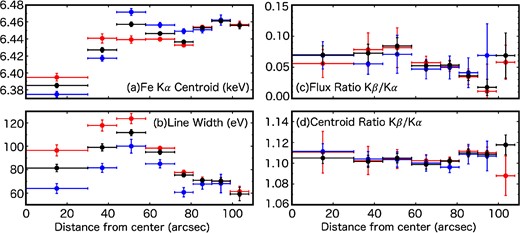
Figure 1 shows a three-color image of Kepler’s SNR, where red, green, and blue indicate the K-shell emission band of Si, O, and Fe, respectively. Thanks to the fine point-spread function (half-power diameter ∼0|${^{\prime\prime}_{.}}$|5) of its High Resolution Mirror Assembly, Chandra successfully resolved a number of small-scale ejecta clumps with different chemical compositions (e.g., Reynolds et al. 2007). Nevertheless, we first investigate one-dimensional radial profiles of the surface brightness, centroid energy, and line width of the Fe Kα emission in order to investigate the overall trend. We divide the entire SNR into eight annulus regions (Regions 1–8), assuming the SNR center to be (|${17^{\rm h}30^{\rm m}41{^{\rm s}_{.}}321}$|, |${-21{^{\circ}}29^{\prime }30{^{\prime\prime}_{.}}510})$|) (Sato & Hughes 2017b). The radius of Region 1 is |${30{^{\prime\prime}_{.}}}$| and the widths of the outer annulus are |${14{^{\prime\prime}_{.}}}$| (for Regions 2–4) and |${9{^{\prime\prime}_{.}}}$| (Regions 5–8). The 4.0–7.7 keV spectrum of the brightest annulus (Region 5) is shown in figure 2. This energy band contains Kα emission of Cr, Mn, Fe, and Ni, and Fe Kβ emission (Park et al. 2013), which are also confirmed in our Chandra spectrum. Therefore, we fit the spectrum with Gaussian models for the five line features plus a power-law continuum. The spectra from all eight regions are simultaneously fitted to link the centroid of Cr, Mn, and Ni among the regions and the Fe Kβ centroid between Regions 6 and 7. All the other parameters (centroid, width, and brightness) for these lines were treated as free parameters among the regions. The fitting was successful with parameters listed in table 2, with χ2 (d.o.f.) of 0.93371 (1089), and the resulting radial profiles are given in figure 3.
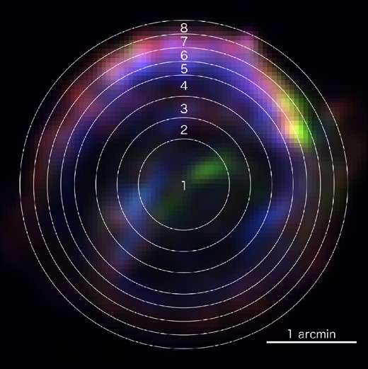
Chandra three-color image of Kepler’s SNR, binned with 3″ and smoothed with a Gaussian kernel of 9″. The scale is in square root. North is up and east is to the left. The red, green, and blue images are made using the energy bands containing Si K emission (1.78–1.93 keV), O K emission (0.50–0.70 keV), and Fe K emission (6.20–6.70 keV), respectively. The white circles indicate where we extract spectra to generate the radial profiles in figure 3. (Color online)
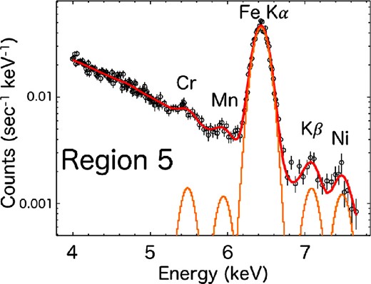
Example spectrum in the 4.0–7.7 keV band, extracted from the brightest annulus Region 5. The red line represents the best-fitting model, and orange Gaussians indicate the contribution of Cr, Mn, Fe, and Ni Kα emission, and Fe Kβ emission. (Color online)
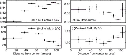
The radial profiles of (a) Fe Kα centroid, (b) 1σ line width, (c) Kβ/Kα flux ratio and (d) Kβ/Kα centroid energy ratio. Error bars represent the 1σ confidence level.
Best-fitting spectral parameters for the radial profile.*
| Line | Centroid (keV) | Width (1σ) (eV) | Brightness† | Centroid (keV) | Width (1σ) (eV) | Brightness† | |
|---|---|---|---|---|---|---|---|
| Region 1 | Region 2 | ||||||
| Cr Kα | 5.484 ± 0.014 | = Fe Kα | 1.0 ± 0.7 | ‡ | = Fe Kα | 1.7 ± 0.7 | |
| Mn Kα | 5.948 ± 0.015 | = Fe Kα | 1.3 ± 0.8 | § | = Fe Kα | 1.8 ± 0.8 | |
| Fe Kα | 6.385 ± 0.003 | 81 ± 3 | 94.7 ± 2.2 | 6.427 ± 0.003 | 99 ± 3 | 95.6 ± 2.1 | |
| Fe Kβ | 7.056 ± 0.034 | = Fe Kα | 6.6 ± 1.4 | 7.081 ± 0.038 | = Fe Kα | 7.0 ± 1.4 | |
| Mn Kα | 7.499 ± 0.012 | = Fe Kα | 4.1 ± 2.1 | ‖ | = Fe Kα | 1.05 ± 2.2 | |
| Region 3 | Region 4 | ||||||
| Cr Kα | ‡ | = Fe Kα | 1.7 ± 0.7 | ‡ | = Fe Kα | 1.5 ± 0.6 | |
| Mn Kα | § | = Fe Kα | 2.9 ± 0.7 | § | = Fe Kα | 1.3 ± 0.7 | |
| Fe Kα | 6.457 ± 0.003 | 112 ± 3 | 99.7 ± 1.9 | 6.446 ± 0.002 | 95 ± 2 | 133 ± 2 | |
| Fe Kβ | 7.135 ± 0.029 | = Fe Kα | 8.4 ± 1.3 | 7.083 ± 0.028 | = Fe Kα | 7.0 ± 1.1 | |
| Mn Kα | ‖ | = Fe Kα | 7.8 ± 2.0 | ‖ | = Fe Kα | 10.4 ± 1.7 | |
| Region 5 | Region 6 | ||||||
| Cr Kα | ‡ | = Fe Kα | 3.2 ± 0.8 | ‡ | = Fe Kα | 3.0 ± 0.7 | |
| Mn Kα | § | = Fe Kα | 3.5 ± 0.8 | § | = Fe Kα | 4.1 ± 0.8 | |
| Fe Kα | 6.436 ± 0.001 | 75 ± 2 | 181 ± 2 | 6.453 ± 0.001 | 71 ± 2 | 159 ± 2 | |
| Fe Kβ | 7.094 ± 0.019 | = Fe Kα | 9.6 ± 1.3 | 7.163 ± 0.024 | = Fe Kα | 5.8 ± 1.2 | |
| Mn Kα | ‖ | = Fe Kα | 12.2 ± 2.0 | ‖ | = Fe Kα | 13.3 ± 1.9 | |
| Region 7 | Region 8 | ||||||
| Cr Kα | ‡ | = Fe Kα | 3.0 ± 0.7 | ‡ | = Fe Kα | 0.2** | |
| Mn Kα | § | = Fe Kα | 2.0 ± 0.7 | § | = Fe Kα | 0.8 ± 0.5 | |
| Fe Kα | 6.461 ± 0.002 | 70 ± 3 | 83.8 ± 1.7 | 6.456 ± 0.004 | 71 ± 2 | 26.1 ± 1.0 | |
| Fe Kβ | ♯ | = Fe Kα | 1.5 ± 1.1 | 7.215 ± 0.062 | = Fe Kα | 1.8 ± 0.9 | |
| Mn Kα | ‖ | = Fe Kα | 6.4 ± 1.6 | ‖ | = Fe Kα | 4.2 ± 1.4 | |
*Errors are at the 1σ confidence level.
†Units of × 10−10 cm−2 s−1 arcsec−2.
‡ |$^,$| § |$^,$| ‖Cr, Mn, and Ni Kα centroid is linked with that in region 1, respectively.
#Fe Kβ centroid in region 7 is linked with that in region 6.
**Error range of the Cr Kα brightness in region 8 is not constrained.
The lowest Fe Kα centroid energy is found at the innermost region (figure 3a), which is somewhat unexpected. Moreover, the measured value (6.385 ± 0.003 keV) is even lower than the theoretical energy of the Kα fluorescence from neutral Fe. This suggests that the Fe emission from the SNR center is substantially redshifted due to the asymmetric distribution of the line-of-sight velocity. This interpretation is also supported by the radial profile of the line width (figure 3b). A relatively narrow emission found at the innermost region is in contrast to Tycho’s SNR, where the largest line width is confirmed at the SNR center, as expected for a uniformly expanding shell (Furuzawa et al. 2009; Hayato et al. 2010; Sato & Hughes 2017a). We also reveal radial trends in the Fe Kβ/Kα flux and centroid ratios, which respectively show lower and higher values at the outer regions (figures 3c and 3d). Details will be discussed in subsection 4.1.
In the case of Kepler’s SNR, the reverse shock dynamics on the north and south sides can be different from each other due to the biased-CSM distribution (e.g., Williams et al. 2012). It would make a difference of the ionization states (Kβ/Kα ratios) between the north and south sides. However, we did not find such a significant difference in radial profiles between north and south (see the Appendix). We therefore assume the same ionization states in one radial profile hereafter.
3.2 Small-scale velocity structure
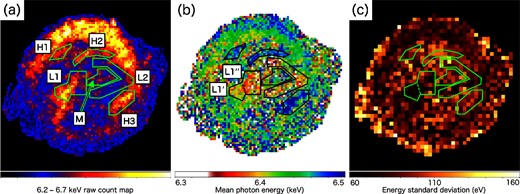
(a) Photon count, (b) mean photon energy (|$\bar{E}$|), and (c) standard deviation (S) maps in the 6.2–6.7 keV band. Each image bin corresponds to 3 × 3 arcsec2 for panels (a) and (b), and 6 × 6 arcsec2 for panel (c). Region names for subsection 3.2 are also shown. (Color online)
For a more quantitative study, we extract spectra from six characteristic regions indicated in figure 4: high-energy regions (H1–H3), low-energy/narrow-line regions (L1, L2), and a region surrounded by the low-energy regions (M). The Fe Kα spectra of Regions H3, L1, and M are compared in figure 5. We fit the 4.0–7.7 keV spectrum of each region with Gaussians (for the emission lines) and a power law (for the continuum), obtaining the best-fitting values given in table 3. The results are generally consistent with the MPE and deviation maps; e.g., the Fe Kα lines of Regions L1 and L2 are indeed lower than 6.4 keV and narrow.
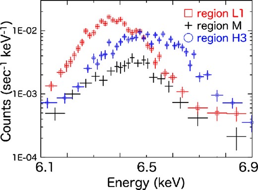
Magnified spectra around the Fe Kα emission (6.1–6.9 keV) of Regions L1 (red), M (black), and H3 (blue). (Color online)
Best-fitting spectral parameters for small characteristic regions.*
| Region | Centroid (keV) | Width (1σ) (eV) | Norm† | Brightness‡ | Centroid (keV) | Width (1σ) (eV) | Norm† | Brightness‡ | |
|---|---|---|---|---|---|---|---|---|---|
| Fe Kα | Fe Kβ | ||||||||
| H1 | 6.483 ± 0.007 | 83 ± 8 | 58 ± 3 | 166 ± 9 | 7.285 ± 0.073 | = Fe Kα | 5 ± 2 | 14 ± 6 | |
| H2 | 6.496 ± 0.007 | 102 ± 9 | 86 ± 4 | 165 ± 8 | 7.185 ± 0.087 | = Fe Kα | 4 ± 3 | 8 ± 6 | |
| H3 | 6.505 ± 0.004 | 108 ± 4 | 179 ± 5 | 200 ± 6 | 7.204§ | = Fe Kα | 5 ± 3 | 6 ± 3 | |
| L1 | 6.381 ± 0.003 | 69 ± 3 | 215 ± 5 | 161 ± 4 | 7.044 ± 0.051 | = Fe Kα | 7 ± 3 | 5 ± 2 | |
| L2 | 6.388 ± 0.005 | 86 ± 6 | 105 ± 4 | 66 ± 3 | 7.001 ± 0.093 | = Fe Kα | 7 ± 3 | 4 ± 2 | |
| M | 6.438 ± 0.008 | 94 ± 9 | 55 ± 3 | 80 ± 4 | 7.056 ± 0.213 | = Fe Kα | 2 ± 2 | 3 ± 3 | |
*Errors are at a 1σ confidence level.
†Units of × 10−7 cm−2 s−1.
‡Units of × 10−10 cm−2 s−1 arcsec−2.
§Error range is not constrained.
4 Discussion
We have investigated both radial trend and small-scale distribution of the Fe K emission characteristics and spatially resolved the red- and blueshifted ejecta components, for the first time. In this section, we aim to constrain the actual line-of-sight velocity of the Fe ejecta from the observed centroid energy in each small region. We should note, however, that the K-shell fluorescence energy depends also on the charge number of Fe ions (Yamaguchi et al. 2014). Therefore, we first investigate the charge population in the shocked ejecta to estimate the average centroid energy of Fe Kα lines at the rest frame. For this purpose, we perform plasma diagnostics in subsection 4.1, and subsequently determine the line-of-sight velocity in subsection 4.2.
4.1 Ionization state of Fe ejecta
Yamaguchi et al. (2014) presented that the Fe Kβ/Kα flux ratio is sensitive to the Fe charge number (or ionization degree), because the fluorescence yields of these lines depend on the number of bound electrons in the 2p and 3p shells. More specifically, strong Kβ emission is expected only from low-ionization plasma where 3p electrons are still bound. We find in figure 3c that the Fe Kβ/Kα flux ratio gradually decreases towards the outer regions, indicating that the average charge number is higher at the outer region. This result is consistent with the fact that the SNR reverse shock propagates inward so that the ejecta in the outer layer get ionized earlier. We also find that the Fe Kβ/Kα centroid energy ratio, which is independent of the kinematic Doppler effect, increases with the distance from the SNR center. This trend is also due to the ionization effect; the fluorescence energy of Fe Kβ emission increases faster than that of Fe Kα emission with respect to the charge number (see table 2 of Yamaguchi et al. 2014).
In figure 6, the Fe Kβ/Kα flux and centroid ratios observed in the eight annular regions (black crosses) are compared with the theoretical values calculated using the atomic data of Yamaguchi et al. (2015). The blue curves assume a single ionization age, net (where ne and t are the electron density and the time elapsed since shock heating), ranging from 1 × 10⁹ to 2 × 1010 cm−3 s. The impact of different electron temperatures are explored for kTe = 3–7 keV, which contains a previously-reported electron temperature of the Fe ejecta in this SNR (∼5 keV: Park et al. 2013). We find that the “one-net” models generally fail to reproduce the observed ratios. This implies the presence of a wider range of plasma conditions, because a lower Kβ/Kα centroid ratio is expected if the Kα and Kβ emission is predominantly originating from the high- and low-ionized component, respectively, as in the case of Tycho’s SNR (Yamaguchi et al. 2014). We thus apply the “two-net” models consisting of net = 108 and 1010 cm−3 s plasmas or net = 109 and 1010 cm−3 s plasmas with various fractions of each component. The red curves in figure 6 indicate the range of the calculated ratios, where a larger fraction of the low-ionized component is assumed at the upper left-hand (higher flux ratio) region. The observed Fe K properties are well explained with this “two-net” assumption.
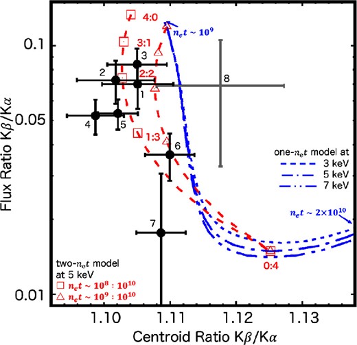
Relationship between the Fe Kβ/Kα centroid ratio (horizontal axis) and flux ratio (vertical axis) measured in the annulus regions (Regions 1–8, indicated in the plot). The error bars represent 1σ confidence. Blue curves indicate theoretically-expected relations for “single-net” plasmas with net values ranging from 109 cm−3 s (upper left-hand side) to 2 × 1010 cm−3 s (bottom right-hand side). Various electron temperatures (3, 5, and 7 keV) are considered. Red dashed curves assume “two-net” models consisting of net = 108 and 1010 cm−3 s plasmas (squares) or net = 109 and 1010 cm−3 s plasmas (triangles). The fractions of each component (defined by the flux contributing to the Fe Kα emission) are also indicated beside the symbols. (Color online)
We find that the values observed in Regions 1–5 can be reproduced when the low-ionization component (net of either 108 or 109 cm−3 s) is responsible for 25%–75% of the Fe Kα flux. On the other hand, the plasmas in Regions 6–8 are dominated by the high-ionization component. It should be noted that the theoretical Fe Kα centroid energy remains almost constant (E ∼ 6400 eV) within the range of net = 108 and 109 cm−3 s and the difference in the Kβ/Kα centroid ratios is mainly owing to the charge-number dependence of the Kβ centroid energy (Yamaguchi et al. 2014). Since the Fe Kα centroid for the net = 1010 cm−3 s plasma is predicted to be ∼6450 eV, we can estimate the rest frame centroid energy of the Fe Kα emission from Regions 1–5 to be (6400 + 6450)/2 ≈ 6425 eV, assuming the responsibility of the low-ionization component is 50%. The estimated variation in the fraction of low-ionization component gives an uncertainty of ∼10 eV.
4.2 Asymmetric structure of Fe ejecta motion
Ejecta velocity in small characteristic regions.
| Region | v sight* (km s−1) | Doppler shift |
|---|---|---|
| H1 | −2700 ± 700 | Blueshift |
| H2 | −3300 ± 700 | Blueshift |
| H3 | −3700 ± 700 | Blueshift |
| L1 | 2100 ± 700 | Redshift |
| (L1″ | 1400 ± 700 | Redshift) |
| (L1″ | 2700 ± 700 | Redshift) |
| L2 | 1700 ± 700 | Redshift |
| M | −600 ± 800 | No shift |
*The statistical and systematic errors are included. Positive velocity represents redshifted ejecta.
Regions H1–H3 show significant blueshift with the velocity of ∼3000 km s−1, whereas Regions L1 and L2 are redshifted with the velocity of ∼2000 km s−1. The apparent “no-shift” in Region M will be discussed later. The absolute values of the line-of-sight velocities of the blueshifted ejecta in Regions H1–H3 are relatively larger than those of the redshifted ejecta in Regions L1 and L2. In addition, Regions H1–H3 are located at larger off-axis angles from the expansion center than Regions L1 and L2, so that the difference between blue- and redshifted ejecta in three-dimensional (3D) space velocity may be even larger. The broader line-width in these regions may also support the higher 3D space velocity of the blueshifted ejecta. It is interesting to note that the blueshifted ejecta in Regions H1–H3 have a clear counterpart in the Fe Kα line flux image (figure 4a) whereas the redshifted ejecta do not; the red portion in Region L1 in the MPE map (figure 4b) does not appear to correspond to the bright structure running across the boundary of Region L1 toward the southeast in the flux image, and there is no characteristic structure in Region L2 in the flux image. The blueshifted ejecta might have been ejected as high-velocity dense clumps like the “Fe knot” in Tycho’s SNR (Yamaguchi et al. 2017), while redshifted ejecta might be an ensemble of relatively uniformly distributed smaller structures, resulting in the diffuse appearance without distinct shape.
On the other hand, the no-shift in the Fe Kα centroid in Region M suggests that red- and blueshifted ejecta are superimposed in this region. More specifically, based on the clumpy and diffuse appearances of the blue- and redshifted ejecta, blueshifted ejecta corresponding to a structure seen in Region M in the Fe Kα line flux image may be superimposed on diffuse redshifted ejecta that are widely distributed over Regions L1, L2, and M. To confirm this idea, we fitted the Fe Kα line spectrum in Region E with two Gaussians; one is responsible for the redshifted ejecta that has the same centroid energy and line width as those of the Fe Kα line in Region L2 (Gaussian 1), and the other is for additional blueshifted ejecta (Gaussian 2). The spectrum is successfully reproduced with this model (figure 7 and the best-fitting values in table 5). The derived vsight for the additional blueshifted component in Region M is comparable with those in Regions H1–H3, or may be slower considering that Region M is located at the center of the remnant and less subject to a projection effect. Figure 8 shows the O band map (0.5–0.7 keV band) contours, which represent the CSM distribution (Katsuda et al. 2015), on the MPE map (figure 4b). A clear morphological coincidence between the dense CSM structure and the shape of the “no-shift region” (Region M) is evident, suggesting that the blueshifted ejecta in Region M would have interacted with the dense CSM on the near side of the SNR and be decelerated. This scenario is supported by the fact that the optical filaments in this region are blueshifted (Blair et al. 1991, 2007). Blair et al. (2007) also showed that the CSM located in Region L1″ are redshifted and the velocity there is close to that at Region M. This fact suggests that the redshifted ejecta in Region L1″ would have interacted with the CSM on the far side, in contrast to the case in Region M. Figure 9 shows a schematic drawing of the Fe ejecta properties in Kepler’s SNR, which summarizes our understanding.
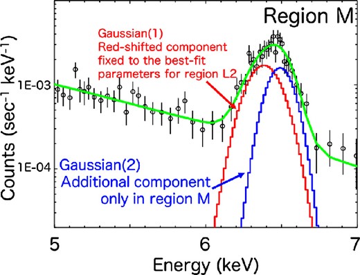
The 5–7 keV spectrum of Region M modeled with a power law and two Gaussians representing the red- and blueshifted Fe Kα emission. The line centroid and width of the former component are fixed to the best-fitting values for Region L2. (Color online)
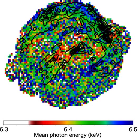
Same color map as figure 4b, with the oxygen band flux image overplotted in black contours. (Color online)
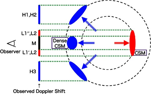
Schematic view of Kepler’s SNR with region name, describing the observed ejecta properties. An observer is at the left. See text for more details. (Color online)
Best-fitting spectral parameters for the simultaneous fitting of Region L2 and M.*
| Region† | Centroid (keV) | Width (1σ) (eV) | Norm‡ |
|---|---|---|---|
| L2 | 6.388 ± 0.005 | 86 ± 6 | 105 ± 4 |
| M(1) | = region L2 | = region L2 | 30 ± 7 |
| M(2) | 6.492 ± 0.019 | 53 ± 25 | 24 ± 6 |
| Region† | Centroid (keV) | Width (1σ) (eV) | Norm‡ |
|---|---|---|---|
| L2 | 6.388 ± 0.005 | 86 ± 6 | 105 ± 4 |
| M(1) | = region L2 | = region L2 | 30 ± 7 |
| M(2) | 6.492 ± 0.019 | 53 ± 25 | 24 ± 6 |
*Errors indicate the 1σ confidence limits.
†M(1) and M(2) represent Gaussian 1 and 2, respectively.
‡Units of × 10−7 cm−2 s−1.
One of the possible reasons that explains the Fe ejecta asymmetricity is the SNR interaction with the asymmetric ambient medium. Recent 3D numerical studies have succeeded in modeling an asymmetric structure similar to that of Kepler’s SNR (e.g., Chiotellis et al. 2012; Toledo-Roy et al. 2014). Toledo-Roy et al. (2014) calculated the SNR models assuming a runaway progenitor scenario proposed by Bandiera (1987). The model assumed that the SN explosion occurred inside an asymmetric CSM density distribution produced by the strong wind of the companion asymptotic giant branch (AGB) star that was running through the ambient Galactic medium with a velocity of 280 km s−1. As a result, the asymmetric bright X-ray structure around the central region as seen in Kepler’s SNR was produced in the simulations (see figure 10 in Toledo-Roy et al. 2014). However, the authors have argued that such a structure is associated with the interaction of the supernova shockwave and the AGB wind. In our results, the Fe distributions in both spatial and velocity spaces have no strong correlation with the CSM distributions except for Region E (see also Burkey et al. 2013). Therefore, the CSM asymmetry does not seem to be a predominant origin of the asymmetric distribution of the Fe ejecta.
Result of the radial profiles of the north (red) and the south (blue). Black points are the same as figure 3. Error bars represent the 1σ confidence level. The spectrum in the south of Region 8 cannot be analyzed due to the lack of statistics. (Color online)
Burkey et al. (2013) argued that the “shadow” in Fe cast by the companion star might be able to produce the Fe ejecta asymmetricity. Recently, García-Senz, Badenes, and Serichol (2012) predicted a hidden hole that remains for centuries in type Ia SNRs that is caused by the interaction of the ejected materials with the companion star (shadow effect) using 3D hydrodynamical simulations (see also Gray et al. 2016). The model shows a cone-like hole structure during the young SNR stage, which would cause SNR asymmetry in both spatial and velocity space. Also, it is notable that the model predicts that the Rayleigh–Taylor instabilities at the outer edge of the hole develop faster than the average growth rate in the other unstable regions of the SNR models. Such an effect can push the ejecta that have high velocities and densities close to the forward shock, and then the model might be able to explain the Fe ejecta asymmetricity in Kepler’s SNR. For example, we show that the redshifted Fe ejecta are located at the center and they are relatively uniformly distributed structures, resulting in the diffuse appearance without distinct shape; on the other hand, the blueshifted Fe ejecta are located at a larger off-angle axis from the center and they have clear shapes. The structure in which the blueshifted components surrounds the redshifted component may indicate the projected hole structure, if the hole faces us.
Another possible cause of the Fe ejecta asymmetricity would be an asymmetric explosion of the progenitor star. In the core of the SN Ia, a large amount of 56Ni (∼0.6 M⊙) are synthesized, and their asymmetric distribution during the SN explosion due to the ignition process and/or some instabilities is expected (e.g., Maeda et al. 2010; Seitenzahl et al. 2013). Yamaguchi et al. (2017) have focused on the “Fe knot” located along the eastern rim of Tycho’s SNR, and attempted to explain the feature based on the explosion mechanism. This approach to understanding the mechanism of the Fe knot formation would be also useful for our discussion of the Fe ejecta asymmetricity. For example, Yamaguchi et al. (2017) discussed asymmetric Fe distribution using the N100 model of Seitenzahl et al. (2013). The model predicted the appearance of some Fe clumps on the outer layer of SNe Ia during the SN explosion. The Fe clumps created in the initial stage are almost freely expanding and are thought to survive until the young SNR stage. Such an effect might cause the Fe distribution seen in Kepler’s SNR. In order to conclude that such an asymmetric explosion is the origin of the Fe ejecta asymmetricity in the remnant, comparing the distribution with that of the other stable iron-peak elements (e.g., Cr, Mn, Ni) is necessary. The Fe clumps ejected asymmetrically are thought to be synthesized in the neutron-rich nuclear statistical equilibrium (n-NSE) layer and be scattered by some instabilities during the explosion. Therefore, the other n-NSE burning products (e.g., Mn and Ni) must be produced in the same region (see figure 13 in Yamaguchi et al. 2017). However, at present, the total X-ray counts in each region are too poor to estimate the element mass from the weak lines (see figure 7). In the future, even longer exposure observations by Chandra or XMM-Newton will be able to reveal it.
5 Conclusions
The kinematic asymmetry of iron-peak elements in the type Ia SNe is key to understanding the explosion mechanism, and studying the ejecta motion of SNRs is useful for approaching the mechanism. In order to know the expansion structure of the Fe ejecta of Kepler’s SNR, we analyzed the Fe K band images and spectra using the Chandra 741.0 ks observation. From the radial profiles of the flux and centroid ratio of Fe Kβ/Kα, we resolved the mixture of multi-net components and found that the reverse shock is now propagating from the edge of the remnant to the center. Combining this estimation of the net and the Fe Kα centroid of each region picked up from the mean photon energy map, we found that there are blueshifted ejecta with the velocity of ∼3000 km s−1, whereas other ejecta near the center are redshifted with the velocity of ∼2000 km s−1. At this time, it is difficult to conclude what the physical process forming the asymmetric Fe motion is. Our results favor the “shadow” of the companion star and/or the asymmetric explosion of the progenitor star as the origin of the Fe ejecta asymmetricity in the remnant. The asymmetric distribution of the CSM could also cause the Fe ejecta asymmetricity, however it hardly explains the lack of strong correlation between the Fe and CSM distributions. In order to reveal the formation of the Fe ejecta asymmetricity in Kepler’s SNR, we believe there is still much that the current X-ray observatories (e.g., Chandra, XMM-Newton) can do in the future. In particular, investigating more detailed kinematics of the Fe and the other iron-peak elements will approach the issues. We hope that additional deep observations of type Ia SNRs such as Kepler’s SNR will be planned in coming cycles.
Acknowledgements
We thank the anonymous referee for comments to improve the manuscript. We also thank Kazuhiro Nakazawa, Satoru Katsuda, Sangwook Park, Asami Hayato, John P. Hughes, and Yoshihiro Furuta for helpful suggestions and discussion. T.K. is supported by the Advanced Leading Graduate Course for Photon Science (ALPS) in the University of Tokyo, and T.S is supported by the Special Postdoctoral Researchers Program in RIKEN. This work is partly supported by the Japan Society for the Promotion of Science (JSPS) KAKENHI Grant Numbers 15K051017 and 16H03983.
Appendix.
Radial profile in the northern and the southern halves
In addition to the non-biased radial profiles discussed in subsection 3.1, we also investigate radial profiles in the northern/southern halves. We fitted all spectra using the same method as subsection 3.1, and the results are given in figure 10. Although the Fe Kα centroid and line width are partly different, the flux ratio and the centroid ratio Kβ/Kα are consistent in both halves. The difference would only be due to the Doppler motion in the line-of-sight direction, not the ionization effect. As a whole, the tendency is the same as the result in subsection 3.1, that the center regions have a smaller Fe Kα centroid and smaller line width, supporting the asymmetric expansion.
The northern/southern difference in the reverse shock dynamics might not be necessary for a runaway progenitor model (e.g., Bandiera 1987). Chiotellis, Schure, and Vink (2012) calculated the models for Kepler’s SNR assuming that the progenitor system was a symbiotic binary moving toward the northwest with a velocity of 250 km s−1. The models produce an asymmetric wind bubble around the progenitor. Then, the forward shock interaction with the wind bubble begins ∼300 yr after the explosion when the forward shock was at a radius of ∼2–3 pc. In this case, the northern/southern asymmetry of the forward shocks grows with time after the encounter. However, the growth rate of the asymmetry on the reverse shocks seems to be much lower than that of the forward shocks (see figure 5 in Chiotellis et al. 2012). This might support our result of nonsignificant difference in the northern/southern radial dependencies of the ionization states.
References
