


Abstract
We searched for precursive soft X-ray flashes (SXFs) associated with optically discovered classical or recurrent novae in the data of five years’ all-sky observations with the Gas Slit Camera (GSC) of the Monitor of All-sky X-ray Image (MAXI). We first developed a tool to measure the fluxes of point sources by fitting the event distribution with a model that incorporates the point-spread function (PSF-fit) to minimize the potential contamination from nearby sources. Then we applied the PSF-fit tool to 40 classical/recurrent novae that were discovered in optical observations from 2009 August to 2014 August. We found no precursive SXFs with significance above the 3 σ level in the energy range of 2–4 keV between td − 10 d and td, where td is the date when each nova was discovered. We obtained the upper limits for the bolometric luminosity of SXFs, and compared them with the theoretical prediction and that observed for MAXI J0158−744. This result could constrain the population of massive white dwarfs with a mass of roughly 1.40 solar mass, or larger, in binary systems.
1 Introduction
Both classical and recurrent novae are triggered by thermonuclear runaways, which last for ∼100 s at the surface of white dwarfs. Subsequently, the optical flux increases by six or more magnitudes, followed by an eventual decline to quiescence (Warner 1995). At the time of thermonuclear runaways, an emission in the ultraviolet to soft X-ray bands that lasts for only a few hours is predicted and is called the “fireball phase” (Starrfield et al. 2008; Krautter 2008). The fireball phase is predicted to happen a few days before the beginning of the optical nova phase, although it has not been detected yet from any nova system.
In fact, MAXI/GSC did discover an extraordinarily luminous soft X-ray flash (SXF) MAXI J0158−744 (Li et al. 2012; Morii et al. 2013). The MAXI J0158−744 system was considered to be in the fireball phase, although there was no association with a usual classical/recurrent nova. This SXF is characterized with a soft X-ray spectrum, a short duration (ΔTd; 1.3 × 10³ s <ΔTd < 1.10 × 10⁴ s), a rapid rise (<5.5 × 10³ s), and a huge peak luminosity of 2 × 1040 erg s−1 in the 0.7–7.0 keV band. Although the characteristics of this flash are very different from those of usual novae, the soft X-ray emission was successfully interpreted as the fireball phase of a new kind of nova on a very massive white dwarf (Morii et al. 2013). Indeed, this hypothesis was further supported with a detailed simulation performed by Ohtani, Morii, and Shigeyama (2014). The soft X-ray emission during the fireball phase is a photospheric emission, and, accordingly, the spectral shape is basically a blackbody. Morii et al. (2013) also concluded that the small increase in the flux observed in the optical counterpart of MAXI J0158−744 did not originate from a photospheric emission as for usual novae, but is due to the emission from the disk around the Be companion star, which is a reprocess, originated from the photospheric soft X-ray emission. Now, unlike MAXI J0158−744, the companion star in the white-dwarf binaries that generate novae is in general not a Be star. Therefore, it is unlikely that any detectable increase in the optical flux would occur during a SXF of a nova, where the companion star is not a Be star.
It has been argued in many theoretical studies that white dwarfs can acquire a mass close to or over the Chandrasekhar limit via differential rotation (e.g., Yoon & Langer 2004; Hachisu et al. 2012) or strong internal magnetic fields (e.g., Das & Mukhopadhyay 2012; Franzon & Schramm 2015). However, the theoretical works have not caught up with the observational discovery of the new type of nova from a very massive white dwarf (MAXI J0158−744; Morii et al. 2013). At the same time, we need more observational samples to study and understand the phenomenon and its background science. Here we present the result of the systematic search for nova explosions from very massive white dwarfs.
In this paper, we perform a systematic search for the fireball phase emission in the soft X-ray band for usual classical/recurrent novae, using the association of optically discovered novae as predicted by Starrfield, Iliadis, and Hix (2008) and Krautter (2008). We should note that SXFs without an optical-nova phase, like MAXI J0158−744, are outside our samples and hence would not be detected in this search. However, intermediate objects that possess both the fireball phase with an SXF emission and an optical nova phase are expected to be found, if such objects are actually present.
2 Observation and analysis
MAXI (Monitor of All-sky X-ray Image: Matsuoka et al. 2009) is an all-sky X-ray monitor, which is operated on the Japanese Experiment Module (KIBO) on the International Space Station (ISS). MAXI carries a Gas Slit Camera (GSC: Mihara et al. 2011; Sugizaki et al. 2011), which scans almost the entire sky every ∼92 min through a long and narrow field of view (FoV) of 1|$_{.}^{\circ}$|5 × 160°. The scan duration for a point source is 40–150 s (Sugizaki et al. 2011). GSC with its gas proportional counters is sensitive for 2–30 keV. From the start of the operation on 2009 August 15 up to the present day, GSC has almost continuously monitored the whole sky. All the data have been stored at the Japan Aerospace Exploration Agency (JAXA) and the Institute of Physical and Chemical Research (RIKEN).
Table 1 shows the classical/recurrent novae discovered in the period from 2009 August 15 to 2014 August 15, taken from the reports of the International Astronomical Union Circulars (IAUC) and Central Bureau Electronic Telegrams (CBET). MAXI/GSC observed these fields of the sky at the period of the discovery in the optical wavelength. Accordingly, MAXI/GSC can search for precursive activity in the X-ray band for these novae.
Forty-four classical/recurrent novae discovered in the optical wavelengths during the five years from 2009 August to 2014 August.
| Nova | RA* | Dec† | Discovery date | Class§ | References‖ |
|---|---|---|---|---|---|
| (°) | (°) | (UT)‡ | |||
| V2672 Oph | 264.582 | − 26.737 | 2009-08-16.515 | CN | IAUC 9064 |
| V5584 Sgr | 277.887 | − 16.319 | 2009-10-26.439 | CN | IAUC 9089 |
| V496 Sct | 280.940 | − 7.612 | 2009-11-08.370 | CN | IAUC 9093, CBET 2008 |
| KT Eri | 71.976 | − 10.179 | 2009-11-25.545 | CN | IAUC 9098 |
| V1722 Aql | 288.541 | +15.276 | 2009-12-14.40 | CN | IAUC 9100 |
| V2673 Oph | 264.921 | − 21.663 | 2010-01-15.857 | CN | IAUC 9111 |
| V5585 Sgr | 271.862 | − 29.012 | 2010-01-20.72 | CN | IAUC 9112 |
| U Sco | 245.628 | − 17.879 | 2010-01-28.4385 | RN | IAUC 9111 |
| V2674 Oph | 261.634 | − 28.827 | 2010-02-18.845 | CN | IAUC 9119 |
| V1310 Sco | 256.531 | − 37.241 | 2010-02-20.857 | CN | IAUC 9120 |
| V407 Cyg | 315.541 | +45.776 | 2010-03-10.797 | SyN | CBET 2199 |
| V5586 Sgr | 268.262 | − 28.205 | 2010-04-23.782 | CN | IAUC 9140 |
| V1311 Sco | 253.805 | − 38.063 | 2010-04-25.788 | CN | IAUC 9142 |
| V1723 Aql | 281.910 | − 3.787 | 2010-09-11.485 | CN | IAUC 9167 |
| V5587 Sgr | 266.943 | − 23.587 | 2011-01-25.86 | CN | IAUC 9196 |
| V5588 Sgr | 272.589 | − 23.092 | 2011-03-27.832 | CN | IAUC 9203, CBET 2679 |
| T Pyx | 136.173 | − 32.380 | 2011-04-14.2931 | RN | IAUC 9205, CBET 2700 |
| V1312 Sco | 253.789 | − 38.635 | 2011-06-01.40 | CN | IAUC 9216, CBET 2735 |
| PR Lup | 223.583 | − 55.084 | 2011-08-04.73 | CN | IAUC 9228, CBET 2796 |
| V1313 Sco | 249.179 | − 41.546 | 2011-09-06.37 | CN | IAUC 9233, CBET 2813 |
| V965 Per | 47.818 | +37.084 | 2011-11-07.75 | CN | IAUC 9247 |
| V834 Car | 162.582 | − 64.113 | 2012-02-26.543 | CN | IAUC 9251, CBET 3040 |
| V1368 Cen | 205.289 | − 58.255 | 2012-03-23.386 | CN | IAUC 9260, CBET 3073 |
| V2676 Oph | 261.529 | − 25.862 | 2012-03-25.789 | CN | IAUC 9259, CBET 3072 |
| V5589 Sgr | 266.367 | − 23.090 | 2012-04-21.01123 | CN | IAUC 9259, CBET 3089 |
| V5590 Sgr | 272.766 | − 27.291 | 2012-04-23.689 | CN | IAUC 9259, CBET 3140 |
| V2677 Oph | 264.983 | − 24.795 | 2012-05-19.484 | CN | IAUC 9260, CBET 3124 |
| V1324 Sco | 267.725 | − 32.622 | 2012-05-22.80 | CN | CBET 3136 |
| V5591 Sgr | 268.107 | − 21.439 | 2012-06-26.5494 | CN | IAUC 9259, CBET 3156 |
| V5592 Sgr | 275.114 | − 27.741 | 2012-07-07.4986 | CN | IAUC 9259, CBET 3166 |
| V5593 Sgr | 274.904 | − 19.128 | 2012-07-16.512 | CN | IAUC 9259, CBET 3182 |
| V959 Mon | 99.911 | +5.898 | 2012-08-07.8048 | CN | IAUC 9259, CBET 3202 |
| V1724 Aql | 283.146 | +0.312 | 2012-10-20.4294 | CN | IAUC 9259, CBET 3273 |
| V809 Cep | 347.020 | +60.781 | 2013-02-02.4119 | CN | IAUC 9260, CBET 3397 |
| V1533 Sco | 263.498 | − 36.106 | 2013-06-03.6146 | CN | IAUC 9260, CBET 3542 |
| V339 Del | 305.878 | +20.768 | 2013-08-14.5843 | CN | IAUC 9258, CBET 3628 |
| V1830 Aql | 285.639 | +3.255 | 2013-10-28.4571 | CN | IAUC 9263, CBET 3691, CBET 3708 |
| V556 Ser | 272.264 | − 11.210 | 2013-11-24.3835 | CN | IAUC 9264, CBET 3724 |
| V1369 Cen | 208.696 | − 59.152 | 2013-12-02.692 | CN | IAUC 9265, CBET 3732 |
| V5666 Sgr | 276.286 | − 22.601 | 2014-01-26.857 | CN | IAUC 9269, CBET 3802 |
| V745 Sco | 268.843 | − 33.250 | 2014-02-06.694 | RN | CBET 3803 |
| V962 Cep | 313.599 | +60.285 | 2014-03-08.7917 | CN | IAUC 9270, CBET 3825 |
| V1534 Sco | 258.945 | − 31.475 | 2014-03-26.8487 | CN | IAUC 9273, CBET 3841 |
| V2659 Cyg | 305.426 | +31.058 | 2014-03-31.7899 | CN | IAUC 9271, CBET 3842 |
*Right ascension.
†Declination.
‡(Year)-(Month)-(Day)
§CN: classical nova; RN: recurrent nova; SyN: symbiotic nova.
‖IAUC: The International Astronomical Union Circulars; CBET: Central Bureau Electronic Telegrams.
We started the data analysis from the event data of MAXI/GSC stored for every day and every camera in the fits format. For every source, we extracted events from a circular sky region centered on the target with a radius of 8°, using mxextract. We also calculated the time variation of the effective area in every 1 s for the point source determined by the slat–slit collimator of MAXI/GSC, using mxscancur. We made good time intervals (GTIs) to include this duration and to remove the duration when the counter was off. We also removed the scans during which the solar paddle of the ISS obscured the FoV of the GSC counter. The selected event data in fits format were converted to root1 format to enhance visualization of the data. For every scan, we measured the flux of the target in units of counts s−1 cm−2 in the 2–4 keV band, using the tool named “PSF-fit.” The details of “PSF-fit” are described in the Appendix. The spectrum file and the corresponding response file were made for every scan by using xselect and mxgrmfgen, respectively.
We made the light curves of the sources listed in table 1 for every GSC scan using the PSF-fit tool from td − 50 d to td + 50 d, where td is the date when each nova was discovered in the optical wavelength. We also calculated the upper limits for the fluxes at the 90% confidence level (C.L.) for the scans with non-detection, using the same tool.
3 Results
For every nova listed in table 2, no significant precursive SXF was found at more than the 3 σ level during the period between td − 10 d and td. Note that in this table, U Sco, V1310 Sco, V5666 Sgr, and V745 Sco as listed in table 1 are removed due to the following reasons. U Sco is removed due to the occasional contamination of the tail of the PSF of Sco X-1. Although the angular distance between them is not so small (2|$_{.}^{\circ}$|4), Sco X-1 is the brightest X-ray source in the entire sky (∼10 Crab), so the contamination sometimes becomes severe. V1310 Sco is also removed due to the contamination of the nearby bright source GX 349+2, which is 0|$_{.}^{\circ}$|8 apart from V1310 Sco. For V5666 Sgr and V745 Sco, there was no GTI of GSC scans during the searched periods.
Results of our search for soft X-ray flashes for the 40 novae in table 1.
| Nova* | N H † | Distance | U.L.‡ | N s § | Reference for distance |
|---|---|---|---|---|---|
| (cm−2) | (kpc) | ave (min–max) | |||
| V2672 Oph | 4.18 × 10²¹ | 19 ± 2 | 2.51 (0.71–4.24) | 22 | Takei et al. (2014) |
| V5584 Sgr | 3.96 × 10²¹ | 6.3 ± 0.5 | 1.20 (0.38–3.28) | 134 | Raj et al. (2015) |
| V496 Sct | 6.81 × 10²¹ | 2.9 ± 0.3 | 2.22 (0.74–4.75) | 45 | Raj et al. (2012) |
| KT Eri | 5.52 × 10²⁰ | 6.6 ± 0.8 | 1.71 (0.61–6.03) | 109 | Imamura and Tanabe (2012) |
| V1722 Aql | 9.14 × 10²¹ | 5 | 1.97 (0.63–6.01) | 112 | Munari et al. (2010) |
| V2673 Oph | 2.84 × 10²¹ | 7.4 | 1.42 (0.43–4.38) | 77 | Munari and Dallaporta (2010) |
| V5585 Sgr | 2.75 × 10²¹ | N/A | 1.76 (0.50–4.36) | 44 | |
| V2674 Oph | 4.12 × 10²¹ | 9 | 1.75 (0.67–3.96) | 30 | Munari, Dallaporta, and Ochner (2010) |
| V407 Cyg | 8.19 × 10²¹ | 2.7 | 1.83 (0.56–4.46) | 52 | Munari, Margoni and Stagni (1990) |
| V5586 Sgr | 9.60 × 10²¹ | N/A | 2.79 (1.21–5.64) | 23 | |
| V1311 Sco | 4.78 × 10²¹ | N/A | 1.98 (0.52–4.44) | 20 | |
| V1723 Aql | 1.23 × 10²² | 6 | 1.76 (0.49–4.97) | 140 | Weston et al. (2016) |
| V5587 Sgr | 4.09 × 10²¹ | N/A | 1.56 (0.30–3.67) | 126 | |
| V5588 Sgr | 5.47 × 10²¹ | 7.6 | 2.15 (0.65–5.67) | 122 | Munari et al. (2015) |
| T Pyx | 1.88 × 10²¹ | 3.5 ± 1 | 1.87 (0.43–8.19) | 35 | Schaefer (2010) |
| V1312 Sco | 5.14 × 10²¹ | N/A | 1.61 (0.47–4.64) | 118 | |
| PR Lup | 4.82 × 10²¹ | N/A | 1.25 (0.39–3.76) | 144 | |
| V1313 Sco | 4.77 × 10²¹ | N/A | 1.09 (0.26–3.71) | 55 | |
| V965 Per | 1.20 × 10²¹ | N/A | 3.56 (1.37–8.18) | 17 | |
| V834 Car | 4.98 × 10²¹ | N/A | 1.49 (0.38–5.09) | 121 | |
| V1368 Cen | 4.30 × 10²¹ | N/A | 1.37 (0.46–3.50) | 47 | |
| V2676 Oph | 3.02 × 10²¹ | N/A | 1.34 (0.36–3.56) | 89 | |
| V5589 Sgr | 3.35 × 10²¹ | N/A | 2.21 (0.47–5.85) | 111 | |
| V5590 Sgr | 2.64 × 10²¹ | N/A | 2.19 (0.70–5.50) | 107 | |
| V2677 Oph | 3.38 × 10²¹ | N/A | 3.46 (0.79–11.27) | 44 | |
| V1324 Sco | 4.35 × 10²¹ | 4.5 | 2.56 (0.79–6.05) | 47 | Ackermann et al. (2014) |
| V5591 Sgr | 4.27 × 10²¹ | N/A | 2.31 (0.61–6.59) | 134 | |
| V5592 Sgr | 1.49 × 10²¹ | N/A | 2.01 (0.72–5.96) | 93 | |
| V5593 Sgr | 6.54 × 10²¹ | N/A | 2.31 (0.66–5.97) | 115 | |
| V959 Mon | 6.29 × 10²¹ | 3.6 | 2.68 (0.71–9.77) | 118 | Shore et al. (2013) |
| V1724 Aql | 1.47 × 10²² | N/A | 2.49 (0.61–7.11) | 133 | |
| V809 Cep | 8.22 × 10²¹ | 6.5 | 1.98 (0.65–5.25) | 93 | Munari et al. (2014) |
| V1533 Sco | 7.42 × 10²¹ | N/A | 2.10 (0.66–4.36) | 84 | |
| V339 Del | 1.36 × 10²¹ | 4.2 | 2.04 (0.64–6.08) | 140 | Shore (2013) |
| V1830 Aql | 1.23 × 10²² | N/A | 3.08 (0.86–8.20) | 128 | |
| V556 Ser | 4.87 × 10²¹ | N/A | 2.54 (0.93–6.70) | 89 | |
| V1369 Cen | 5.84 × 10²¹ | 2.4 | 2.58 (0.74–8.95) | 83 | Shore et al. (2014) |
| V962 Cep | 3.30 × 10²¹ | N/A | 2.72 (1.11–11.86) | 125 | |
| V1534 Sco | 3.88 × 10²¹ | 13 | 1.77 (0.79–4.24) | 22 | Joshi et al. (2015) |
| V2659 Cyg | 4.92 × 10²¹ | N/A | 2.27 (0.73–6.13) | 124 |
*U Sco, V1310 Sco, V5666 Sgr, and V745 Sco listed in table 1 are removed (see text).
†Total Galactic H i column density toward the source as the average of the values obtained by the Leiden/Argentine/Bonn (LAB) map (Kalberla et al. 2005) and the DL map (Dickey & Lockman 1990), calculated using the HEASARC website 〈http://heasarc.gsfc.nasa.gov/cgi-bin/Tools/w3nh/w3nh.pl〉.
‡90% C.L. upper limit for the flux in the 2–4 keV band for each scan in units of 10−2 counts s−1 cm−2. The average (minimum and maximum) fluxes among Ns scans are shown.
§Number of GSC scans in the searched period.
We then calculated the 90% C.L. upper limit for the fluxes in every scan for the sources in units of counts s−1 cm−2 in the 2–4 keV band (table 2). Since the expected times of the SXFs are unknown, the upper limits given in the table are the averaged values for all the scans between td − 10 d and td, as well as the minimum and maximum. From these averaged flux upper limits, we calculated the upper limits for the bolometric luminosity of the sources, using the interstellar absorption NH and the distance (table 2), and assuming the temperature of blackbody spectrum for the fireball-phase emission. Figure 1 shows the derived upper limits.
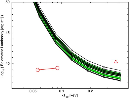
90% C.L. upper limits for bolometric luminosity of the fireball phase of classical/recurrent novae searched for in this work (see table 2). In the conversion from the observed GSC flux in the 2–4 keV band (counts s−1 cm−2) to the unabsorbed bolometric luminosity (erg s−1), a blackbody spectrum is assumed, and the interstellar absorption NH and distance listed in table 2 are used. For the sources with unknown distance, we assumed 5 kpc as a typical distance for Galactic sources. The upper limits for the sources with known and unknown distances are shown in black and green lines, respectively. Horizontal and vertical axes are the temperature of blackbody assumed in the flux conversion in keV and the logarithm of the bolometric luminosity, respectively. The theoretical prediction of the fireball phase (Starrfield et al. 2008) is given in red circle points connected with a solid line, to be compared with the derived upper limits, where the left and right circle points correspond to the emission in the fireball phase of white dwarfs with 1.25 and 1.35 solar masses respectively. The red triangle point is the observed value for the fireball phase of MAXI J0158−744 (Morii et al. 2013).
4 Discussion and conclusion
If SXFs are associated precursively with optical novae, if the spectrum and flux are similar to those of MAXI J0158−744, and if the nova is located at the typical distance of 5 kpc, then MAXI/GSC should detect these flashes at a high significance (see figure 1), as long as the FoV of GSC covers the direction during the SXF. MAXI/GSC usually scans a specific direction every 92 minutes. Hence, the probability that MAXI/GSC detects an SXF depends on the duration of the SXF.
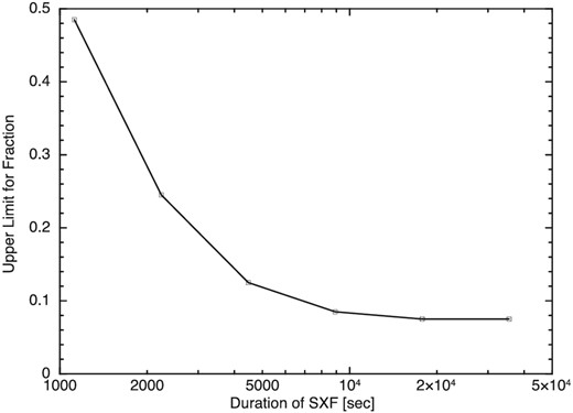
90% C.L. upper limit for the fraction of novae associated with an SXF at the fireball phase (R) as a function of the given duration of SXFs in seconds (see text).
In figure 1, the fireball phase observed for MAXI J0158−744 is located at the extension of theoretical prediction (Starrfield et al. 2008). This supports that the SXF observed on MAXI J0158−744 is the emission from the fireball phase. The mass of the white dwarf of this source is estimated to be at least 1.35 solar mass. Furthermore, by naively drawing a straight line connecting the two points of 1.35 solar mass (the right red circle) and MAXI J0158−744 (red triangle), the crossing point between this line and the average of the lines of the upper limits implies a lower limit for the mass of white dwarfs for which SXFs are detectable with MAXI/GSC. Assuming that the mass of MAXI J0158−744 is at the Chandrasekhar limit of white dwarfs (1.44 solar mass), the mass of a white dwarf that is located at the crossing point is estimated to be about 1.40 solar mass. Therefore, the upper limit for the fraction in figure 2 can be alternatively interpreted as the upper limit for the population of white dwarfs in binary systems whose masses are about 1.40 solar mass or larger. The population of very massive white dwarfs is important for estimating the rate of type Ia supernovae. Our result could give a constraint for this population.
Future observations with MAXI/GSC will detect more SXFs from novae in the fireball phases. In addition, the wide-field MAXI mission currently being planned (Kawai et al. 2014) would improve the detection efficiency of SXFs and would increase the sample of SXFs and very massive white dwarfs. In the light of these prospects, the theoretical study of the fireball-phase emission of novae on very massive white dwarfs, especially from 1.35 solar mass to near the Chandrasekhar limit, is encouraged.
We thank the members of the MAXI operation team. We also thank J. Shimanoe for the first search for transients from optical novae. K. Sugimori, T. Toizumi, and T. Yoshii kindly offered us good help in developing PSF-fit. We are grateful to S. Ikeda on ISM, who advised on the statistical treatment of the data analysis. This work was partially supported by the Ministry of Education, Culture, Sports, Science and Technology (MEXT), under Grant-in-Aid for Science Research 24340041.
Appendix. Flux measurement by using the point-spread function: PSF-fit
X-ray fluxes of point sources are usually measured with aperture photometry, and the standard processing for the MAXI data also does this. The MAXI light curves obtained with this method are published in the archive on the RIKEN website2 In the standard MAXI data processing, the source and background regions to extract events are usually selected as simple circular and annular regions in the sky coordinates, respectively. When the point-spread functions (PSFs) of nearby sources interfere with these regions, the circular regions centered on these nearby sources are excluded. If a target source is located in a severely crowded region like the Galactic plane, measurement of the flux based on such a simple selection of the regions is inadequate, because the PSF of a target overlaps with those of nearby sources and because the area of the background region free from contamination of the nearby sources becomes too small to obtain adequate statistics.
In this work, we developed a tool to measure the fluxes for the point sources by fitting an event distribution around a target with a model that incorporates the PSFs of the target and nearby sources. Both X-ray and non-X-ray backgrounds are also taken into account in this model. We name this tool “PSF-fit.” Below is a detailed description of PSF-fit.
We use the event distribution in the detector coordinate rather than the sky coordinate, because the shape of a PSF is best described in the detector coordinate. In this coordinate, the shape of a PSF is given by a triangular-shaped function in the time (scan) direction, whereas that in the anode wire direction is given by a Gaussian shape (Sugizaki et al. 2011). The triangular shape is well calibrated (Morii et al. 2011). The width of the Gaussian shape (sigma) depends on counters, the position of the anode direction, and the high voltage (HV; 1650 V or 1550 V). We calibrated this dependence by measuring the width of the Gaussian shape for the bright point sources Crab nebula, GRS 1915+105, and Cyg X-1, for the energy bands of 2–4 and 4–10 keV. Thus, we obtained a well-calibrated PSF model.
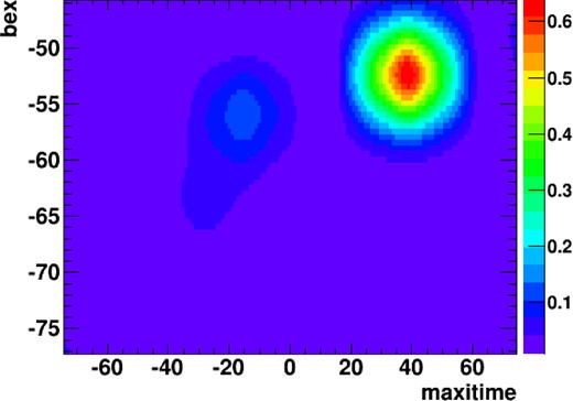
We select events from a rectangular region in the detector coordinate, where the width of the time (scan) direction is determined to be three times the width of the base side of the triangular shape. That of the anode direction is set to be 16 sigma of the Gaussian shape. As a result, these widths vary in every scan. We then add a constraint for these widths so that the rectangular region cannot exceed a circular sky region with a radius of 8°, which is the radius of the event extraction at the beginning of the analysis (section 2). Figure 3 shows an example of the event distribution in the detector coordinates to be used for the PSF-fit. It is for V5586 Sgr on a scan at the modified Julian day (MJD) 55340 with a camera (ID = 0) in the 2–4 keV band.
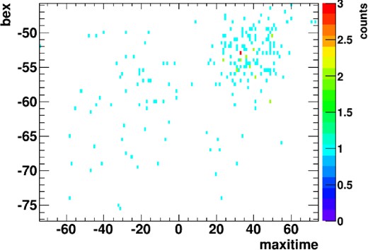
Event distribution in the detector coordinates extracted for the PSF-fit for V5586 Sgr on a scan at MJD 55340 by a camera (ID = 0) in the 2–4 keV band. The horizontal and vertical axes are the relative time(s) from 2010-05-24 15:34:14 (UT) and bex (mm), respectively. The color scale shows the number of events in a bin.
When a target is located in a crowded region like the Galactic plane, there are many nearby sources; some sources are always bright enough to be detected by MAXI/GSC, while some are usually faint and have the potential to become bright above the threshold of MAXI/GSC sensitivity. For almost any region in the sky, MAXI/GSC is the only X-ray detector that monitors these sources; then it is impossible to determine a priori which sources are detectable and which are not. However, we must select which source is necessary to be included in the model for the PSF-fit. We approach this problem as follows.
We pick candidates for the nearby sources to be included in PSF-fit from the catalog used in the Nova search system (Negoro et al. 2015). The area for selecting these candidates is the rectangular region in the detector coordinates as described above and the outer marginal region with half the width of the base side of the triangular shape for the time direction and three sigma of the Gaussian shape for the anode direction. This marginal region for selecting the nearby sources is necessary to account for the contamination of PSFs of sources out of the fitting region, within which the events are extracted (figure 3). Figure 4 demonstrates the positions of the nearby candidate sources listed in the catalog in the example case, as well as the region for the event extraction (fitting) and outer marginal regions.
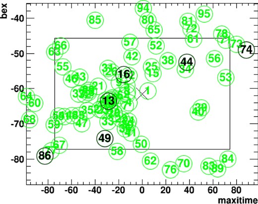
Positions of the nearby source candidates and the selected sources are shown with numerical labels in green and black colors, respectively. The cross label at the center is the position of the target, V5586 Sgr. The scan time and camera are the same as in figure 3. The area used for the PSF-fit is displayed as a rectangular region, which is the same area as that in figure 3.
The nearby sources included in the PSF-fit (black labels in figure 4) are selected with the measure of the Bayesian information criterion (BIC: Schwarz 1978) from the candidates (green labels in figure 4) as follows. First, we fit the event distribution with the simplest model that includes only the background, and calculate the BIC. Next, we include one nearby source among all the nearby candidate sources into the model function, and fit the events with this model and calculate the BIC. We then identify the best nearby source with the minimum BIC as the first selected nearby source. If this minimum BIC is larger than that of the previous BIC obtained by the fit that includes only the background, which means that no nearby source is necessary to improve the fit, then the model selection for the nearby sources is completed. Otherwise, we include this source in the final model, then proceed to the next step. In the next step, we include another nearby source among the rest of the nearby sources, and repeat the above procedure. We stop this procedure when the BIC reaches the minimum. Finally, we add the target source in the final model. Figure 4 demonstrates the positions of nearby sources selected with this model selection, and these are used for the fitting process.
Figures 5, 6, and 7 show an example of the best-fit model obtained with the PSF-fit tool; they show the model function and the projection onto the time and anode directions, respectively.
Best-fit function obtained with the PSF-fit for the same region as in figure 3. The values of the best-fit function are shown in units of counts s−1 mm−1 (color bar).


To demonstrate the efficacy of the PSF-fit, we present figure 8. It shows a light curve of a moderately bright and stable source 4U 1746−37. Due to a periodic contamination of the tail of the PSF of a nearby bright source, the light curve available on the RIKEN website is disturbed with a periodic artificial modulation caused by the precession of the ISS (top panel). With the PSF-fit, this modulation effect is clearly removed (bottom panel).
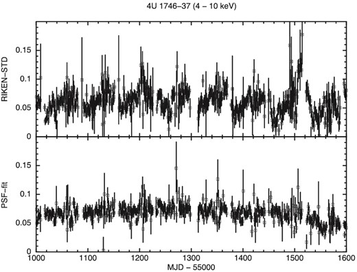
Light curves of 4U 1746−37 in the 4–10 keV band in one-day bins in units of counts s−1 cm−2. The horizontal axis is in days (MJD − 55000). The top panel shows the light curve in the data archive at the RIKEN website, whereas the bottom panel is that obtained with the PSF-fit.
References
