


Abstract
We present an overview of two-dimensional (2D) core-collapse supernova simulations employing a neutrino transport scheme by the isotropic diffusion source approximation. We study 101 solar-metallicity, 247 ultra metal-poor, and 30 zero-metal progenitors covering zero-age main sequence mass from 10.8 M⊙ to 75.0 M⊙. Using the 378 progenitors in total, we systematically investigate how the differences in the structures of these multiple progenitors impact the hydrodynamics evolution. By following a long-term evolution over 1.0 s after bounce, most of the computed models exhibit neutrino-driven revival of the stalled bounce shock at ∼200–800 ms postbounce, leading to the possibility of explosion. Pushing the boundaries of expectations in previous one-dimensional studies, our results confirm that the compactness parameter ξ that characterizes the structure of the progenitors is also a key in 2D to diagnosing the properties of neutrino-driven explosions. Models with high ξ undergo high ram pressure from the accreting matter onto the stalled shock, which affects the subsequent evolution of the shock expansion and the mass of the protoneutron star under the influence of neutrino-driven convection and the standing accretion-shock instability. We show that the accretion luminosity becomes higher for models with high ξ, which makes the growth rate of the diagnostic explosion energy higher and the synthesized nickel mass bigger. We find that these explosion characteristics tend to show a monotonic increase as a function of the compactness parameter ξ.
1 Introduction
The explodability of massive stars depends sensitively on the presupernova structures (e.g., O'Connor & Ott 2011; Ugliano et al. 2012; Couch & Ott 2013; Sukhbold & Woosley 2014). For low-mass progenitors with an O–Ne–Mg core, the neutrino mechanism works successfully to explode in one-dimensional (1D) simulations because of the tenuous envelope (Kitaura et al. 2006). For more massive progenitors with an iron core, multi-dimensional (multi-D) effects such as neutrino-driven convection (e.g., Bethe 1990; Herant et al. 1994; Burrows et al. 1995; Janka & Müller 1996; Müller & Janka 1997) and the standing accretion shock instability (SASI: Blondin et al. 2003; Foglizzo et al. 2006, 2007; Ohnishi et al. 2006; Blondin & Mezzacappa 2007; Iwakami et al. 2008, 2009; Fernández & Thompson 2009; Guilet & Foglizzo 2012; Hanke et al. 2012; Foglizzo et al. 2012; Couch 2013; Fernández et al. 2014; see Foglizzo et al. 2015 for a review) have been suggested to help the onset of the neutrino-driven explosion. Recently this has been confirmed by a number of self-consistent two- and three-dimensional (2D and 3D) simulations (e.g., Buras et al. 2006; Ott et al. 2008; Marek & Janka 2009; Bruenn et al. 2013; Suwa et al. 2010, 2014; Müller et al. 2012a, 2013; Takiwaki et al. 2012, 2014; Hanke et al. 2013; Dolence et al. 2015; Bruenn et al. 2014; Müller & Janka 2015; see Mezzacappa et al. 2015; Janka 2012; Burrows 2013; Kotake et al. 2012 for recent reviews). Up to now, the number of these state-of-the-art models amounts to ∼40 covering the zero-age main sequence (ZAMS) mass from 8.1 M⊙ (Müller et al. 2012a) to 27 M⊙ (Hanke et al. 2013).
Based on stellar evolutionary calculations, on the other hand, hundreds of core-collapse supernova (CCSN) progenitors are available now, depending on a wide variety of the ZAMS mass, metallicity, rotation, and magnetic field (e.g., Nomoto & Hashimoto 1988; Woosley & Weaver 1995; Woosley et al. 2002; Woosley & Heger 2007; Heger et al. 2000, 2005; Limongi & Chieffi 2006). These huge sets of CCSN progenitors, aided by development of high-performance computers and numerical schemes, make systematic numerical study of CCSNe possible.
By performing general-relativistic (GR) 1.5D simulations for over 100 presupernova models using a leakage scheme, O'Connor and Ott (2011) were the first to point out that the postbounce dynamics and the progenitor-remnant connections are predictable basically by a single parameter: the compactness of the stellar core at bounce (see also O'Connor & Ott 2013). Along this line, Ugliano et al. (2012) performed 1D hydrodynamic simulations for 101 progenitors of Woosley, Heger, and Weaver (2002). By replacing the protoneutron star (PNS) interior with an inner boundary condition, they followed an unprecedentedly long-term evolution over hours to days after bounce in spherical symmetry. Their results also lent support to the finding by O'Connor and Ott (2011) that the compactness parameter is a good measure to diagnose the progenitor-explosion and the progenitor-remnant correlation (see also Pejcha & Thompson 2015; Perego et al. 2015).
Joining in these efforts but going beyond the previous 1D approach, we perform neutrino-radiation hydrodynamics simulations in two dimensions using the whole presupernova series (101 solar-metallicity models, 247 ultra metal-poor models, and 30 zero-metal models) of Woosley, Heger, and Weaver (2002). Without the excision inside the PNS, we can self-consistently follow a long-term evolution starting from the onset of core-collapse, bounce, neutrino-driven shock-revival, until the revived shock comes out of the iron core. The goal of our 2D models is not to determine the very final fate of a massive star (which requires 3D-GR models with detailed transport scheme, e.g., Kuroda et al. 2015), but to study the systematic dependence of the progenitors’ structure on the shock revival time, diagnostic explosion energy, mass of the remnant object, and nucleo- synthetic yields. To this end, this study is the first attempt in the multi-D context.
Section 2 describes the numerical setup, including explanation of our numerical scheme (subsection 2.1), the structure of the solar-metallicity 101 progenitors (subsection 2.2), and a discussion on the effects of our choice of the outer boundary (subsection 2.3). Our results start from section 3, where we first focus on the hydrodynamics evolution of the 101 solar-metallicity progenitors, and then move on to analyze the results in terms of the compactness parameters (section 4). Section 5 presents results of the 247 ultra-metal-poor and the 30 zero-metal progenitors. We summarize our results and discuss their implications in section 6.
2 Numerical setup
2.1 Numerical scheme
The numerical methods employed are based on those in Takiwaki, Kotake, and Suwa (2014). Our 2D models are computed on a spherical polar grid of 384 non-equidistant radial zones from the center up to 5000 km. Our spatial grid has a finest mesh spacing drmin = 0.5 km at the center and dr/r is better than 1.8% at r > 100 km. Our hydrodynamic scheme requires two ghost cell layers just above the outer boundary. We fix the density and velocity in the ghost cells to be the values there of the progenitor models (see subsection 2.3 for the effects of the outer boundary). We set 128 equidistant angular zones covering 0 ≤ θ ≤ π so that the angular resolution is 1|$_{.}^{\circ}$|4. We employ the equation of state (EOS) by Lattimer and Swesty (1991) with a compressibility modulus of K = 220 MeV (LS220). For the calculations presented here, self-gravity is computed by a Newtonian monopole approximation and our code is updated, from the ZEUS-MP (Hayes et al. 2006) code used in Takiwaki, Kotake, and Suwa (2014), to use a high-resolution shock capturing scheme with an approximate Riemann solver from Einfeldt (1988). As described in Nakamura et al. (2014a), we take into account explosive nucleosynthesis and the energy feedback into hydrodynamics by solving a 13 α-nuclei network including 4He, 12C, 16O, 20Ne, 24Mg, 28Si, 32S, 36Ar, 40Ca, 44Ti, 48Cr, 52Fe, and 56Ni. The nuclear energy compensates for energy loss via endothermic decomposition of iron-like NSE nuclei to lighter elements (see the appendix of Nakamura et al. 2014a for more details).
To solve the spectral transport of electron and anti-electron neutrinos (νe and |${\bar{\nu }}_{\rm e}$|), we employ the isotropic diffusion source approximation (IDSA: Liebendörfer et al. 2009). We take a ray-by-ray approach, in which the neutrino transport is solved along a given radial ray assuming that the hydrodynamic medium for the direction is spherically symmetric (e.g., Buras et al. 2006). Although one needs to deal with the lateral transport more appropriately (e.g., Sumiyoshi et al. 2015; Dolence et al. 2015), this approximation is useful because of the high computational efficiency in parallelization, which allows us to explore a more systematic progenitor survey based on the radiation hydrodynamics models than ever before in this study. Regarding heavy-lepton neutrinos (|$\nu _x = \nu _{\mu }, \nu _{\tau }, \bar{\nu }_{\mu }, \bar{\nu }_{\tau }$|), we employ a leakage scheme to include the νx cooling via pair, photo, and plasma processes (see Takiwaki et al. 2014 for more details). To induce non-spherical instability, we add initial seed perturbations by zone-to-zone random density variations with an amplitude less than 1%.
There is still a debate about whether explosions are obtained more easily in low-resolution simulations than in high-resolution ones and how much resolution is needed to obtain a convergence (e.g., Radice et al. 2015). In appendix 1, we discuss the resolution dependence of our 2D results.
2.2 Progenitor models
The investigated solar-metallicity progenitors with iron cores (Woosley et al. 2002) are given in 0.2 M⊙ steps between 10.8 M⊙ (s10.8) and 28.2 M⊙ (s28.2), further from 29 M⊙ (s29) up to 40 M⊙ (s40) in 1.0 M⊙ steps, and a 75 M⊙ model (s75); 101 progenitors in total. The structure of these stars, such as the density profiles and the pre-collapse mass distributions, has been already described in Ugliano et al. (2012). Here, for convenience, we show the mass distribution of some selected models at a pre-collapse stage and the time of core bounce (figure 1). Before bounce, the distribution varies from model to model, especially at the outer radius. The mass distribution of the collapsing core dynamically changes after the onset of collapse, but at bounce, the mass distributions remain almost identical within ∼2 × 107 cm among the different progenitor models (bottom panel).
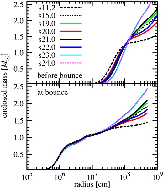
Mass distribution of some selected models at a pre-collapse stage (top panel) and at the time of core bounce (bottom). (Color online)
Figure 2 compares ξM estimated at M = 1.5 M⊙ (ξ1.5,cb), 2.0 M⊙ (ξ2.0), and 2.5 M⊙ (ξ2.5). Note that ξ1.5,cb is estimated at the time of core bounce, whereas the others are directly estimated from the progenitor data. All of these profiles show a similar trend, for example a high compactness bump in the 22–26 M⊙ mass range. Zigzag variations of the compact parameter can be seen for all the lines with the different choice of M, although the amplitude becomes smaller for ξM with larger M. Among all the 101 models, the s11.2 progenitor has the smallest value of the compactness parameter, which is easily seen for the choice of ξ1.5,cb (filled circles). The quantities of the compactness parameters for some representative models are listed in table 1. It includes ξ1.5 from the pre-collapse data and 15 M⊙ progenitors from Woosley and Weaver (1995, WW15) and Woosley and Heger (2007, WH15) as a reference. Metal-deficient progenitors are discussed in section 5.

Three choices of the compactness parameters ξM as a function of ZAMS mass. They are estimated at M = 1.5 M⊙ (ξ1.5,cb), 2.0 M⊙ (ξ2.0), and 2.5 M⊙ (ξ2.5) from top to bottom. Note that ξ1.5,cb is estimated at the time of core bounce as in the previous studies. The others are from pre-collapse data and enhanced by a factor of three for comparison. Model s75 is out of this plot but has ξ1.5,cb = 2.0, ξ2.0 = 0.17, and ξ2.5 = 0.11.
Variations of the compactness parameters from the solar-metallicity progenitors (Woosley et al. 2002).
| Model | ξ1.5,cb | ξ1.5 | ξ2.0 | ξ2.5 |
|---|---|---|---|---|
| s11.2 | 0.300 | 0.195 | 0.014 | 0.005 |
| s15.0 | 1.546 | 0.862 | 0.298 | 0.149 |
| s19.0 | 1.761 | 0.911 | 0.374 | 0.194 |
| s20.0 | 1.414 | 0.671 | 0.187 | 0.127 |
| s21.0 | 2.000 | 0.971 | 0.455 | 0.215 |
| s22.0 | 1.766 | 0.868 | 0.258 | 0.165 |
| s23.0 | 2.617 | 1.000 | 0.720 | 0.434 |
| s24.0 | 2.583 | 0.998 | 0.721 | 0.427 |
| s30 | 1.880 | 0.938 | 0.394 | 0.222 |
| s40 | 2.402 | 0.990 | 0.427 | 0.263 |
| s75 | 2.004 | 0.890 | 0.168 | 0.112 |
| WW15 | 0.765 | 0.592 | 0.194 | 0.085 |
| WH15 | 1.220 | 0.871 | 0.335 | 0.181 |
2.3 Boundary condition
Our simulation domain is limited within the radius of 5000 km so that we can reduce computational cost and carry out 2D self-consistent simulations for the 378 progenitors. This relatively small spatial domain (5000 km), however, might affect the hydrodynamics evolution long after bounce. To clarify this, we check the effects of the outer boundary by estimating the mass accretion rate at different radii. We focus on the mass accretion rate because it predominantly affects the explosion properties, as we will discuss later.
In figure 3, we show the mass accretion history of the three progenitor models with the same ZAMS mass (15 M⊙): WW15 (Woosley & Weaver 1995) (top panel), WH15 (Woosley & Heger 2007) (middle panel), and s15 (Woosley et al. 2002) (bottom panel), respectively. Following Müller and Janka (2015), we estimate the mass accretion rate at the radius of 500 km in figure 3. The radius of the outer boundary (Rout) is taken either at 5000 km or at the more distant radii 500000 km (top panel), 10000 km (middle panel), or 100000 km (bottom panel), respectively. Note that the shock revival is not obtained in the WW15 model that is computed in 1D, whereas the shock revival is obtained at t400 = 688–691 ms and 556–571 ms in the 2D simulations for the WH15 and s15 models, respectively. In the 2D models, the mass accretion rate is only shown before the shock revival (e.g., middle and bottom panels of figure 3) because the mass accretion rate at 500 km can be affected by the non-radial motions of the expanding shock.
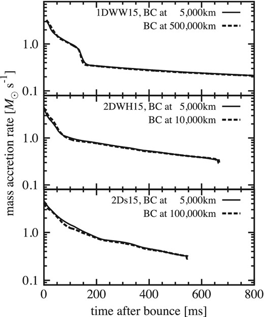
Mass accretion rate of 15 M⊙ progenitor models with outer boundaries at different radii. The lines given by 2D simulations of the WH15 model (middle panel) and s15 model (bottom) are truncated when the shock touches 500 km at tpb ∼ 670 ms, and ∼550 ms, respectively. 1D simulations of the WW15 model (top) do not present shock revival. The difference in the boundary position does not affect the mass accretion rate in all the chosen progenitors.
From figure 3, it can be seen that the mass accretion rate (before the shock reaches the radius of 500 km) is very similar for models with different Rout. It should be noted that the mass accretion rate of the WW15 model shows a sudden drop from 0.8 M⊙ s−1 to 0.3 M⊙ s−1 at tpb ∼ 150 ms (tpb; postbounce time), then gradually decreases to 0.2 M⊙ s−1. This is in a good agreement with the previous results using the same progenitor model (e.g., figure 1 in Murphy & Burrows 2008 and figure 1 in Hanke et al. 2012). All of these facts support that our boundary conditions imitate well the density structure out of the boundary of these three 15 M⊙ models and the boundary effect is not significant for these models.
However, what if there existed a large number of progenitors that would have shell interfaces with sharp density gradients beyond our computational domain (5000 km)? Figure 4 shows the position of the shell interfaces for all the solar-metallicity models employed in our study. Here we define the radius of the silicon (Si) layer at the position where the most abundant element changes from silicon to oxygen (O). Out of the 101 models, we identified 29 models that have the Si/O interface at a radius between 5000 km and 10000 km (horizontal dotted lines). For these models having the shell interfaces above 5000 km, we conduct 1D simulations and plot the mass-accretion rate history in figure 5 to examine the effects of the outer boundary positions. In each model, we vary the position of the outer boundary, either at the radius of 5000 km (shown by solid lines) or at 10000 km (dotted lines).
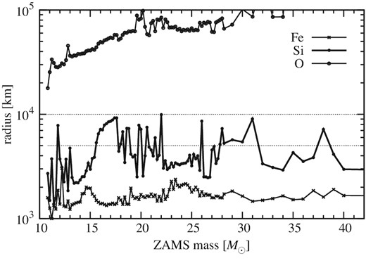
Radius of Fe core surface, Si/O interface, and top of O layer for solar-metallicity models.
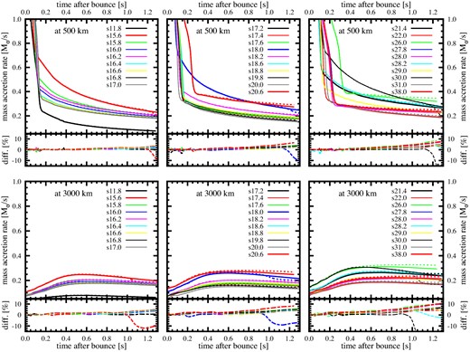
Comparison of the mass accretion rate between 1D models with the outer boundary at radii of r = 5000 km (|$\dot{M}_5$|, solid lines) and 10000 km (|$\dot{M}_{10}$|, dotted). Twenty-nine solar-metallicity models which have the Si/O interface between the radii of 5000 km and 10000 km are shown (see also figure 4). Top: the mass accretion rate estimated at r = 500 km, representing the accretion onto a stalling shock front. Bottom: as the top panels, but estimated at r = 3000 km, representing the accretion rate onto an expanding shock front in 2D models. Relative differences between the models with the two different outer boundary positions |$(\dot{M}_{10} - \dot{M}_5)/\dot{M}_5$| are presented in the lower panel of each plot in percentage. (Color online)
From each panel of figure 5, it can be seen that all of the examined models with the outer boundary at r = 5000 km show very small differences (less than a few percent) from those with the boundary at r = 10000 km before tpb ∼ 0.9 s. In this epoch, the material initially located at r > 5000 km is still at r > 3000 km and the boundary effect is almost negligible. After tpb ∼ 0.9 s, the material initially outside the radius of 5000 km begins passing through the radius of r = 3000 km. Among the 29 progenitors (with shell interfaces above 5000 km, see also figure 4), only three models show a remarkable feature in the mass accretion rate. As shown in the bottom panels of figure 5, s15.6 (a red dotted line in the left panel), s18.0 (a blue dotted line in the middle panel), and s30.0 (a black thin-dotted line in the right panel) with the outer boundary at r = 10000 km show a sudden drop (≳10%) at tpb ∼ 1.0 s, followed by a drop of the accretion rate in the top panels at tpb ∼ 1.2 s. This decrease of the accretion rate in these three models is caused by a density jump at the Si/O interface initially located at the radius r > 5000 km, which cannot be taken into account by the models with the outer boundary at r = 5000 km. In contrast to the models s15.6, s18.0, and s30.0, 10% level increases are observed in the models s20.6, s26.0, s28.0, and s38.0. This is because these models have a relatively high density envelope, for which our choice of the boundary position (at 5000 km) underestimates the mass accretion rate compared to that at 10000 km. There might be such models with a high density envelope in the remaining 72 progenitors other than the four of the 29 progenitors discussed here.
To quantify the boundary effects on these models, we perform 2D simulations for the s38.0 model in the following way. Using the same setups as our fiducial model, the density out of the maximum shock radius is manually changed when the shock reaches 3000 km. We find that increase (decrease) of the density by 10% results in a 2.8% (0.53%) change of the diagnostic energy and negligibly small difference of the PNS mass (<0.03%) at the time when the shock reaches the outer boundary at 5000 km. This is simply because of a small mass accretion rate (<0.3 M⊙ s−1) at this phase and a short period until the simulations are terminated when the shock reaches the outer boundary. Thus, we conclude that the boundary effects on the mass accretion rate in the late postbounce phase are not influential to our systematic study.
3 Results
For all the 101 solar-metallicity models (and also the additional 277 models discussed in section 5), the bounce shock stalls in a spherically symmetric manner, and only after that do we observe a clear diversity of the multi-D hydrodynamics evolution in the postbounce (pb) phase. Figures 6 and 7 show a snapshot of the entropy distribution for 18 selected solar-metallicity models at tpb = 400 ms. For some less massive progenitors (e.g., model s11.2 in figure 6a), the shock reaches close to the outer boundary of the computational domain with developing pronounced unipolar and dipolar shock deformations. At this time, the shock of the most massive progenitor (s75.0 in figure 7i) reaches an average radius of 〈r〉 ∼ 1000 km, whereas the shock of s24.0 (in figure 6i) still wobbles around at 〈r〉 ∼ 200 km. This demonstrates that the ZAMS mass is not a good criterion to diagnose the possibility of explosion.
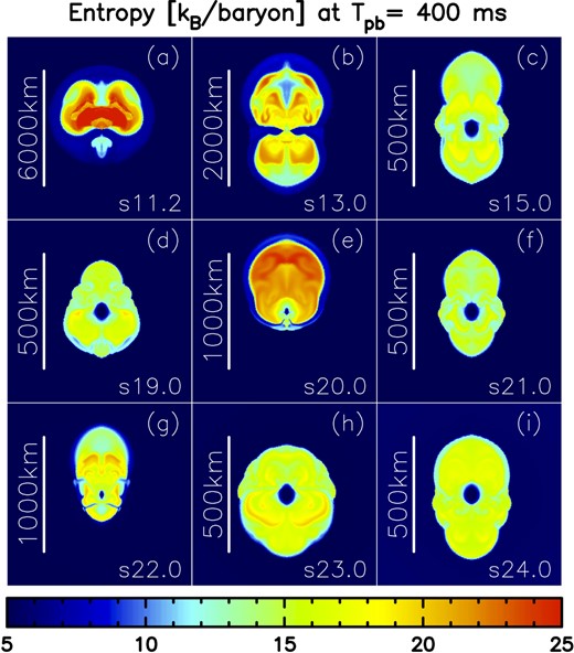
Entropy distributions in units of kB per baryon for nine selected models at tpb = 400 ms. Shown are models s11.2 (a) to s24.0 (i), from top left to bottom right. Note the different scale in each panel. (Color online)

As figure 6 but for models s25.0 (a) to s75.0 (i), from top left to bottom right. (Color online)
This is more clearly visualized in figure 8, showing the time evolution of average shock radii for six models in the mass range between 19.0 M⊙ and 24.0 M⊙. The shock revival is shown to occur earlier for s20.0 (red line) and s22.0 (blue line) compared to the lighter progenitors s19.0 (green line) and s21.0 (black line). Comparing with figure 2, it can be seen that the compactness parameter [equation (1)] is smaller for s20.0 and s22.0 in the chosen mass range. The smaller compactness is translated into smaller mass accretion rate onto the stalled bounce shock. For model s20.0 (ξ2.0 = 0.19, red line in figure 8), the relatively earlier shock revival (∼100 ms postbounce) coincides with the sharp decline of the accretion rate (dashed red line). After that, the accretion rate gradually decreases to ∼0.1 M⊙ s−1 until t400 = 420 ms; at this time the revived shock has expanded to an average radius of 〈r〉 = 400 km. Here, t400 is a useful measure to qualify the vigor of the shock revival (e.g., Hanke et al. 2012). On the other hand, model s21.0 has high compactness (ξ2.0 = 0.46), which leads to the high accretion rate (black dashed line in figure 8). It takes ∼500 ms for the sloshing shock of model s21.0 (black solid line in figure 8) to gradually turn into a pronounced expansion later on and 700 ms to arrive at 〈r〉 = 400 km (t400 = 700 ms).
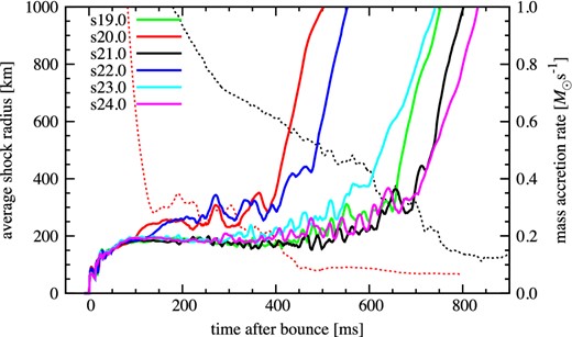
Average shock radii (thick solid lines) and mass-accretion rate of the collapsing stellar core at 500 km (thin dashed lines) for some selected models. (Color online)
Note in figure 8 that the correlation between the compactness and t400 is rather weak. In appendix 2, we attempt to find the alternative compactness parameter by which the correlation is slightly improved.
The gravitational mass of the PNS and the diagnostic explosion energy1 are also shown in figures 9 and 10 as a function of postbounce time. Here, the PNS is defined by the region where the density ρ > 1011 g cm−3. The PNS mass is almost converged in our simulation time and the value at the final simulation time t = tfin has a clear correlation with the compactness parameter. In fact, the PNS masses become smaller for models with smaller compactness parameter (s20.0 drawn with a red line and s22.0 in blue) and bigger for models with higher compactness (s23.0 in sky blue and s24.0 in magenta), and the other two models (s19.0 in green and s21.0 in black) have intermediate values.
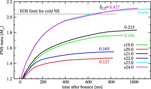
Time evolution of central PNS mass for the same models as in figure 8. The compactness parameter ξ2.5 is labelled beside each line. The horizontal dotted line represents the maximum mass of a cold neutron star of the LS220 EOS. (Color online)
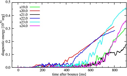
As figure 9, but of the diagnostic energy of the explosion. (Color online)
In figure 9, the horizontal dotted line represents the maximum gravitational mass (2.04 M⊙) of a cold neutron star (NS) for the LS220 EOS employed in this work. As can be seen, the PNS masses of our most “compact” models [e.g., s23.0 (sky blue line) and s24.0 (magenta line)] exceed the limit. Here it should be noted that the upper threshold is for a cold NS, whereas the PNS soon after bounce is still hot. At this phase, the contribution of thermal pressure to the maximum mass cannot be neglected, so that the maximum mass of the hot PNS is bigger than that of a cold NS (O'Connor & Ott 2011; Hempel et al. 2012). Based on a systematic 1D GR simulation with approximate neutrino transport, O'Connor and Ott (2011) showed that the maximum gravitational mass of the hot PNSs, which is bigger for models with high compactness, ranges from 2.1 M⊙ (ξ2.5, cb = 0.20)2 to 2.5 M⊙ (1.15). From figure 7 in O'Connor and Ott (2011), one can read that the maximum gravitational mass for models with ξ2.5, cb = 0.4 (corresponding to the highest ξ in our solar-metallicity model series) is ∼2.2 M⊙, which is bigger than that of the most massive PNS in our 101 solar-metallicity models (MPNS = 2.16 M⊙ for s23.4 model with ξ2.5 = 0.4273; see also figure 14). In their 1D GR study, a model with ξ2.5, cb > 0.4 leads to BH formation at tpb ≲ 1 s. For a given BH-forming progenitor model, the BH formation timescale might be delayed in our 2D exploding models because the shock expansion would possibly make the mass accretion onto the PNS smaller. Although multi-D GR simulations with elaborate neutrino transport scheme are needed to unambiguously clarify this issue, the above exploratory discussions lead us to speculate that BH formation is less likely to affect the systematic features obtained in our solar metallicity models. We will comment further on the possible effects of BH formation in section 5, including for metal-deficient progenitors.
Regarding the diagnostic energy of the explosion (figure 10), it is still increasing at t = tfin and its converged value is difficult to infer from our simulations. The time when the diagnostic energy turns upward corresponds to the time of shock revival (t400). We define its increasing rate as |$\dot{E}_{\rm dia} \equiv E_{\rm dia}(t=t_{\rm fin})/(t_{\rm fin} - t_{400})$| in units of 1051 erg s−1 and find that it tends to become higher for models with high compactness (0.754, 1.12, and 1.44, for s22.0, s23.0, and s24.0, respectively). This also indicates that the diagnostic energy of the high-ξ models would become higher later on. Note that in previous 1D studies with a simplified neutrino heating and cooling scheme (O'Connor & Ott 2011) or with the excision inside the PNS (Ugliano et al. 2012), the relation between the compactness and these explosion properties could not be determined in a self-consistent manner.
We investigate the postbounce shock evolution in more detail for three specific models: s11.2, s15.0, and s27.0. The density profile of model s11.2 falls rapidly off with radius and the compactness parameter ξ2.0 = 0.014 is one of the smallest values among the 101 progenitors, whereas models s15.0 and s27.0 have relatively high compactness (ξ2.0 = 0.298 and 0.326), casting a more extended envelope out to the iron core (see figure 1 for the s15.0 model). Color-coded panels in figure 11 show the different postbounce evolutions for s11.2 (left), s15.0 (middle), and s27.0 (right). Model s11.2 explodes rather early (t400 = 150 ms), and convective activity as well as the oscillations of the shock are moderate before the onset of the explosion (see the bottom left panel). Note in the bottom panels that the anisotropic velocity vaniso (upper), and the normalized pressure perturbation Δp (lower), are defined respectively as |$v_{\rm aniso} = \sqrt{\langle \rho [(v_r - \langle v_r \rangle )^2 + v_{\theta }^2]\rangle /\langle \rho \rangle }$| and |$\Delta p = \sqrt{ \langle p^2 \rangle - \langle p \rangle ^2} /\langle p\rangle$|, where 〈A〉 represents the angle average of quantity A (e.g., Takiwaki et al. 2012; Kuroda et al. 2012).
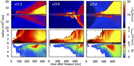
Time–space diagrams of specific entropy (kB/baryon, kB is the Boltzmann constant), anisotropic velocity (cm s−1), and pressure perturbation for models s11.2 (left), s15.0 (middle), and s27.0 (right). Top: the specific entropy along the north (upper panels) and south poles (lower). Bottom: time evolution of the anisotropic velocity vaniso (upper) and the normalized pressure perturbation Δp (lower) in the post-shock region (see the text for details). (Color online)
For model s15.0 with a higher compactness parameter, sloshing motions of the shock are more clearly visible (middle panels of figure 11). These features regarding the dominance of the SASI over neutrino-driven convection for high-ξ models are quantitatively consistent with those observed in previous 2D simulations with a more detailed neutrino transport scheme (e.g., Müller et al. 2012a). The accreting flows receive an abrupt deceleration near the bottom of the gain region, below which the regions are convectively stable. A strong pressure perturbation forms there (seen, in the lower part of the bottom middle panel in figure 11, as a boundary between the regions colored in white and deep blue at a radius of r ≲ 100 km after tpb ∼ 100 ms). In the so-called advective acoustic cycle (see, e.g., Foglizzo et al. 2015 for a review), the pressure perturbations subsequently propagate outward before they hit the shock. This leads to the formation of the next vortices (e.g., yellow regions behind the shock in the vaniso plot). These features, as previously identified, are natural outcomes of the SASI and neutrino-driven convection (e.g., Fernández et al. 2014 and references therein). When the residency timescale becomes long enough compared to the neutrino-heating timescale in the gain region due to these multi-D effects, the runaway shock expansion initiates at tpb ∼ 500 ms (t400 = 556 ms) for this model.
Here we emphasize that the use of the leakage scheme, together with the omission of inelastic neutrino scattering on electrons, is likely to facilitate artificially easier explosions (Takiwaki et al. 2014). Another caveat is GR effects that cannot be treated in our Newtonian simulations. Discrepancies between our Newtonian models and GR models might become remarkable, especially for progenitors with high compactness, because our simulations show that the high-compactness models leave more massive PNSs. Comparing model s27.0 (ξ2.5 = 0.232) for example, the GR model in Müller, Janka, and Heger (2012a) presents more rapid revival of the shock (t400 ∼ 205 ms) than our Newtonian model (t400 = 432 ms). According to Müller, Janka, and Marek (2012b), GR models lead to higher luminosities and mean energies of neutrinos and therefore to larger heating efficiencies in the gain layer, which is favorable to an explosion. For models with moderate compactness parameters, we should note that some key hydrodynamic features in the postbounce phase (such as the onset time of shock revival t400) are rather similar between our models and the Garching models based on Hanke et al. (2013) [t400 = 640 vs. 580 ms for model s18.4 (ξ2.5 = 0.188), 320 vs. 400 ms for s19.6 (0.119), 540 vs. 560 ms for s21.6 (0.181), 460 vs. 460 ms for s22.4 (0.200), respectively, e.g., H.-T. Janka 20133].
4 CCSN properties and compactness
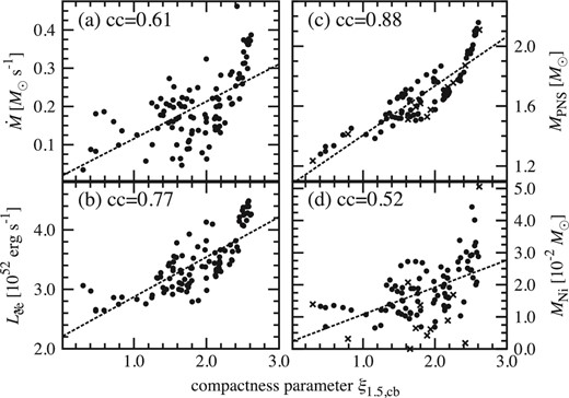
Resultant supernova properties from our 101 simulations as a function of the compactness parameter ξ1.5,cb. Left: (a) mass accretion rate |$\dot{M}$|, and (b) electron neutrino luminosity |$L_{{\nu}_{\rm e}}$|, estimated at time of shock revival t400. Right: (c) mass of PNS MPNS, and (d) mass of nickel MNi in outgoing unbound material, at final time of our simulations tfin. Dashed lines present linear fits with correlation coefficient denoted in each panel. In the right panels, failed models which cannot carry the shock to the outer boundary during our simulation time are shown by crosses and excluded when we estimate the correlation coefficient.
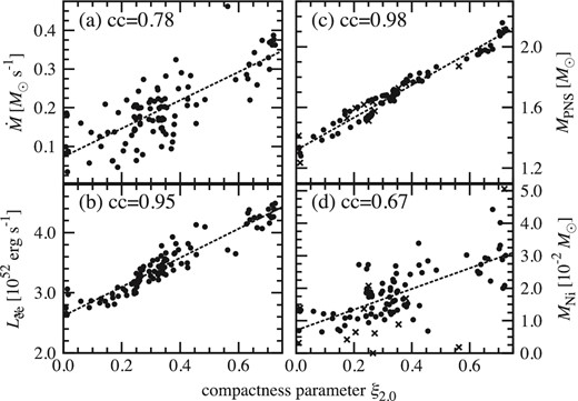
As figure 12 but as a function of ξ2.0.

As figure 12 but as a function of ξ2.5.
For most of our models (89 models), tfin is defined as the time when the maximum shock radius touches the outer boundary. In the remaining 12 models, the shock of model s25.0 has not yet reached the outer boundary within our simulation time (tsim = 1.5 s). The other 11 models are stopped during tsim because the density near the outer boundary of the computation domain goes below the lowest value covered by the EOS table. Fortunately, the shock revival occurs in these 11 models before we stopped the simulations, so that we can measure |$\dot{M}$| and |$L_{\nu _{\rm e}}$| at t = t400. These incomplete models are not taken into account when we estimate the correlation coefficients for MPNS and MNi at t = tfin. Note that it is technically challenging to extend the EOS table smoothly to the non-NSE regime where our 13-species alpha network needs to also be consistently treated between the two regimes. We leave this for future work.
Ugliano et al. (2012) were the first to show that various quantities shown in our figures 12–14 are not a monotonic function of the ZAMS mass. We confirm it in our 2D simulations and find that these values are nearly in linear correlation with the compactness parameters. Furthermore, we point out that the correlation becomes higher for the choice of ξ2.0 or ξ2.5 compared to ξ1.5, cb. This can be interpreted as follows: the core of high-ξ models is surrounded by high-density Si/O layers and the mass accretion rate therefore remains high long after the stalled shock has formed (figures 13a and 8). This makes the PNS mass of the high-ξ models heavier (figure 13c). Due to the high accretion rate, the accretion neutrino luminosities become higher for models with high ξ (figure 13b; see also O'Connor & Ott 2013). As a result, we obtain a stronger shock revival powered by the more intense neutrino heating, which makes the amount of synthesized nickel bigger (figure 13d).
The diagnostic energy of the explosion for the 101 models is in the range ∼0.2–0.7 × 1051 erg, and is still increasing at the final time of our simulation (see figure 10). To obtain a converged value of the diagnostic energy, we need to perform a very long-term simulation including special care around the smooth transition of the EOS to the non-NSE regime, which is beyond the scope of this work. Instead of the converged value, we estimate the growth rate of the diagnostic energy |$\dot{E}_{\rm dia}$| defined in section 3 and plot it in figure 15. Both the diagnostic energy and its growth rate are moderately correlated with the compactness parameter.
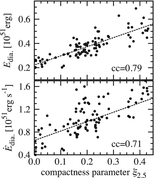
The diagnostic energy of the explosion at t = tfin (top panel) and its growth rate (bottom) as a function of ξ2.5.
5 Metal-deficient progenitors
In this section we move on to discuss the results of metal-deficient progenitors. The ultra metal-poor models of 10−4 Z⊙ contain 247 models with a mass increment of 0.2 M⊙ between 11 and 65 M⊙, and a 75 M⊙ model. The masses of the zero-metallicity progenitors are 11 to 40 M⊙ at every 1.0 M⊙ (30 models in this series).
Figure 16 compares ξ2.5 for these low metallicity models with that of the solar-metallicity models (figure 2). Since the metal-deficient models experience no mass loss during the stellar evolution, the compactness of the metal-poor stars is shown to be much higher for ≳30 M⊙ than that of the solar-metallicity models.
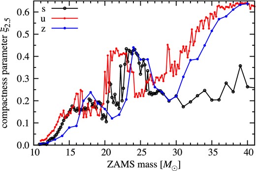
Compactness parameters ξ2.5 of all progenitors as a function of ZAMS mass. Labels s, u, and z denote solar-Z⊙, ultra metal-poor 10−4 Z⊙, and zero metallicity, respectively. (Color online)
Figure 17 shows the mass accretion rate |$\dot{M}$| (top panel) and the electron neutrino luminosity |$L_{{\nu}_{\rm e}}$| (bottom) as a function of the compactness parameter ξ2.5. These two quantities are estimated at the time of shock revival t400. Regardless of the different initial metallicity, the two quantities show a similar increasing trend. In particular, the electron neutrino luminosity is well fitted (the correlation coefficients ≥0.90) by a linear line. Some of the ultra–metal-poor progenitors with high ξ2.5 (>0.45, which do not appear in solar-metallicity models) present a very high accretion rate and neutrino luminosity above the linear trend.
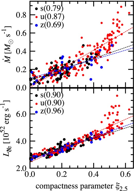
Mass accretion rate |$\skew4\dot{M}$| (top panel) and electron neutrino luminosity |$L_{{\nu}_{\rm e}}$| (bottom) as a function of the compactness parameter ξ2.5. These two quantities are estimated at time of shock revival t400 for all models. The dashed lines present the linear fit with the correlation coefficient denoted in each panel for each progenitor type. (Color online)
Figure 18 shows the PNS mass MPNS (top panel) and the mass of the synthesized nickel MNi in the outgoing unbound material (bottom) as a function of the compactness parameter ξ2.5. These two quantities are estimated at the final time of our simulations tfin. All of the models again show a similar increasing trend. Crosses in the top panel of figure 18 represent the models in which the revived shock did not reach the outer boundary during our simulation time (t = 1.5 s).4 We exclude all the unsuccessful (non-exploding) models shown by the crosses in the top panel of figure 18 when we estimate the correlation coefficients.
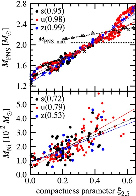
Mass of PNS (MPNS, top panel) and mass of nickel in outgoing unbound material (MNi, bottom) as a function of the compactness parameter ξ2.5. These two quantities are estimated at the final time of our simulations (t = tfin). Failed models which cannot carry the shock to the outer boundary during our simulation time are shown by crosses and excluded when we estimate the correlation coefficient. The horizontal dotted line in the top panel shows the maximum mass of cold NS for LS220 EOS (2.04 M⊙). The another dotted line in the top panel is a linear fit of the triangles, the maximum PNS masses of BH-forming models in O'Connor and Ott (2011); see the text for details. (Color online)
The central PNS of the models in the upper right corner of figure 18 would finally collapse to form a black hole (BH), although our Newtonian code cannot follow such dynamical behavior. Triangles in the top right panel of figure 18 represent the maximum PNS masses estimated by O'Connor and Ott (2011) in which the same progenitor models (Woosley et al. 2002) and the same EOS (LS220) as in this study were examined by their 1D GR code. The dotted curve (MPNS, max = 0.52 ξ2.5 + 2.01) is a linear fit to their results. Our models above the dividing line should be predominantly affected by general relativity and such models cannot be treated appropriately by our Newtonian code.
The fraction of the progenitor models which leave PNS more massive than MPNS, max is 104/378 ∼ 28%. Most of them belong to the u-series (98/104), the ZAMS mass of which is bigger than 32.2 M⊙. Adopting the Salpeter initial mass function to weight the ZAMS mass gives |$\int _{32.2\,M_\odot }^{75\,M_\odot } m^{-2.35} dm / \int _{10\,M_\odot }^{75\,M_\odot } m^{-2.35} dm \sim 15$|%. Although the majority of the PNSs in our 2D models are less than the maximum mass of PNS, we need to perform GR simulations (e.g., O'Connor & Ott 2011; Müller et al. 2012a; Kuroda et al. 2012) in order to elucidate the fate of the high-ξ metal-poor stars.
6 Conclusions and discussion
We have presented an overview of 2D core-collapse supernova simulations employing the neutrino transport scheme by the IDSA scheme. We studied 101 solar-metallicity, 247 ultra–metal-poor, and 30 zero-metal progenitors covering zero-age main sequence mass from 10.8 M⊙ to 75.0 M⊙. Using the 378 progenitors in total, we systematically investigated how the differences in the structures of these multiple progenitors impact the hydrodynamics evolution. By following a long-term evolution over 1.0 s after bounce, most of the computed models exhibited neutrino-driven revival of the stalled bounce shock at ∼200–800 ms postbounce, leading to the possibility of explosion. Pushing the boundaries of expectations in previous one-dimensional studies, our results confirmed that the compactness parameter ξ that characterizes the structure of the progenitors is also a key in 2D to diagnosing the properties of neutrino-driven explosions. Models with high ξ undergo high ram pressure from the accreting matter onto the stalled shock, which affects the subsequent evolution of the shock expansion and the mass of the protoneutron star under the influence of neutrino-driven convection and the standing accretion-shock instability. We have shown that the accretion luminosity becomes higher for models with high ξ, which makes the growth rate of diagnostic energy higher and the synthesized nickel mass bigger. We have found that these explosion characteristics tend to show a monotonic increase as a function of the compactness parameters ξ.
Our simulations are limited in space (r < 5000 km) and time (t ≤ 1.5 s). The simulations are terminated before the diagnostic energies are saturated. Later on, neutrino energy deposition would get smaller with time as the neutrino luminosity as well as post-shock density becomes smaller. Further global simulation, taking account of the gravitational energy of an envelope and nuclear energy released via the recombination process behind the shock, is necessary to determine the final explosion energy (figure 15). Moreover, the finding of this study should be reexamined by 3D models (Hanke et al. 2012; Dolence et al. 2013; Couch 2013; Couch & O'Connor 2014; Nakamura et al. 2014b), in which neutrino transport is appropriately solved (see the discussions in Hanke et al. 2013; Takiwaki et al. 2014; Nagakura et al. 2014; Mezzacappa et al. 2014). It is also important to study the impacts of the precollapse non-spherical structures (e.g., Arnett & Meakin 2011) on fostering the shock revival (e.g., Couch & Ott 2013). To get a more accurate amount of the synthesized nickel and other isotopes, a post-process calculation with a larger nuclear network is needed. In the longer term, wide-range long-term 3D full-scale GR simulations are needed to unambiguously clarify the critical ξ parameter, below or above which neutron stars or black holes will be left behind.
In this work we have reported our results only for progenitors from one modeling group. We are currently conducting the same sort of CCSN simulations for sets of progenitors from other groups, including a variety of metallicity, rotation, and magnetic fields, which will be presented in a forthcoming work.
We thank F. K. Thielemann, M. Liebendörfer, R. M. Cabezón, M. Hempel, and K.-C. Pan for stimulating discussions and for their kind hospitality during our research stay at Basel in 2014 February. We are also grateful to S. Yamada and Y. Suwa for informative discussions. Numerical computations were carried out in part on the XC30 and general common use computer system at the Center for Computational Astrophysics, CfCA, the National Astronomical Observatory of Japan, Oakleaf FX10 at Supercomputing Division in the University of Tokyo, and on the SR16000 at YITP in Kyoto University. This study was supported in part by Grants-in-Aid for Scientific Research from the Ministry of Education, Science, and Culture of Japan (Nos. 23540323, 23340069, 24103006, 24244036, and 26707013) and by the HPCI Strategic Program of Japanese MEXT.
Appendix 1. A numerical resolution
Numerical resolution should be taken as high as possible in order to accurately capture hydrodynamics processes in computational fluid dynamics. In state-of-the-art CCSN simulations, especially in multi-D models, however, high numerical resolution drastically increases the numerical cost, and full convergence has not yet been obtained even in simplified simulations.
Hanke et al. (2012) investigated the resolution dependence in their 2D and 3D models using 11.2 and 15 M⊙ progenitors with a parameterized neutrino heating and cooling scheme. In most of the 2D models, better angular resolution led to easier explosion, although some of them do not obey this trend. On the other hand, Couch (2013) investigated a 15 M⊙ progenitor employing the same simple neutrino scheme as in Hanke et al. (2012), and found that 2D explosions are delayed for models with higher numerical resolution. More recently, Takiwaki, Kotake, and Suwa (2014) computed 2D and 3D models for an 11.2 M⊙ progenitor with an energy-dependent neutrino transport scheme and concluded that higher numerical resolutions led to slower onset of the shock revival in both 2D and 3D.
In our fiducial 2D runs, the angular resolution (Δθ) is taken as 1|$_{.}^{\circ}$|4 (128 angular zones to cover 0 ≤ θ ≤ π). In this appendix, we briefly discuss the resolution dependence, in which we compare the results with the fiducial resolution with those with high resolution (Δθ = 0|$_{.}^{\circ}$|7 with 256 angular zones).
Figure 19 shows the time evolution of the average shock radii for two progenitors, s11.2 and s15.0. In both, it is shown that the shock revival is delayed for the high-resolution models (thin lines). The difference of t400, t1000, and t2500 (the time when the average shock radius arrives at 400 km, 1000 km, and 2500 km, respectively) are 30.4% (13.1%), 29.0% (2.9%), and 6.8% (3.1%) for model s11.2 (s15.0). The relatively large difference of t400 may reflect that the shock revival time is more likely to be affected by stochastic matter motions driven by neutrino-driven convection and the SASI.
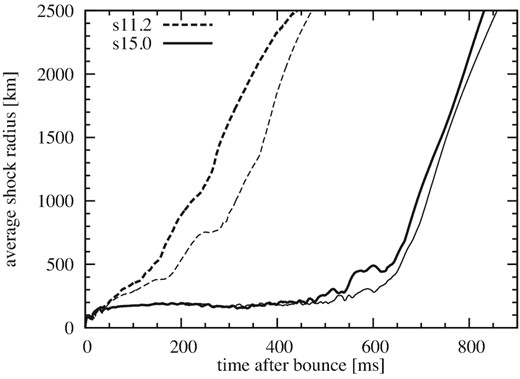
Comparison between different resolution models. Average shock radii as a function of time relative to bounce for the s11.2 and s15.0 models are shown. The shock revives more rapidly in the fiducial resolution models (thick lines) than in high resolution models (thin lines).
The evolution of the diagnostic energies is presented in figure 20. Comparing them at t = t1000 and t2500, the differences between the fiducial and high-resolution models are 22.7% (9.8%) and 28.9% (13.9%) for the s11.2 (s15.0) model. The difference is bigger in model s11.2, which has a small compactness parameter and is weakly exploding, than in model s15.0.
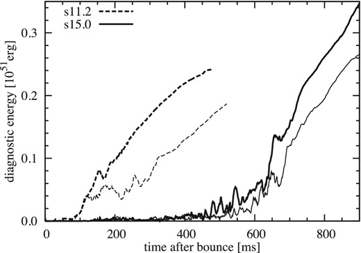
As figure 19 but for the evolution of the diagnostic energies of the explosion.
Our fiducial resolution does not give well-converged results, at least for model s11.2. The systematic behavior that we found, as shown in figure 13, for example, might be subject to change quantitatively. At least, our 2D results showing that higher numerical resolutions lead to slower evolution of the shock radius and the diagnostic explosion energy are consistent with Couch (2013) and Takiwaki, Kotake, and Suwa (2014). A systematic resolution study including a detailed comparison between different numerical codes, schemes, and setups should be done urgently, which we leave for future work.
Appendix 2. Time of shock revival
Our systematic 2D CCSN simulations demonstrate that the ξ parameter is a good diagnostic to infer the progenitor–remnant and progenitor–explosion connections. However, the time of shock revival (t400) shows a large scatter and weaker correlation with the compactness parameter. Figure 21 shows t400 for three kinds of compactness parameters and we obtain low correlation coefficients (0.45–0.54). This may partly come from the stochasticity of the nonlinear growth of SASI and convection, seeded by initial random perturbations, which affects the subsequent shock evolution. Another possibility is that our definition of the compactness parameters might be inappropriate to characterize t400. In this appendix, we attempt to find a more appropriate form of the compactness parameter to characterize the shock revival time.
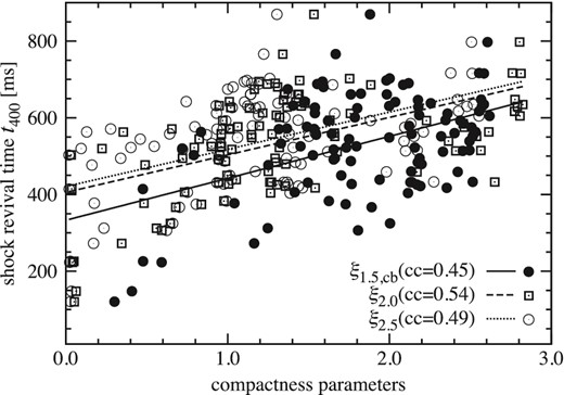
Time of shock revival t400 for three kinds of the compactness parameters. ξ2.0 and ξ2.5 are calibrated by arbitrary factors.
Figure 22 presents t400 as a function of the ratio ξSi+Si/O/ξFe. The concept of this alternative parameter is as follows. The compactness parameter defined at the surface of the iron core (ξFe) is a measure to predominantly determine the core neutrino luminosity, whereas ξSi+Si/O is a measure of the density decline in the outer layer. So we expect that the smaller ratio would lead to an easier explodability. As shown in figure 22, this alternative indicator gives a correlation coefficient of 0.66, which is better than the 0.49 estimated from ξ2.5. To enhance the predictive power, we should more carefully analyze how the compactness parameters are related to the core/accretion luminosity, and the density jump at the Si/O interface. We leave this for future work.
![Time of shock revival t400 estimated as a function of the alternative compactness parameter [e.g., equation (2)].](https://oup.silverchair-cdn.com/oup/backfile/Content_public/Journal/pasj/67/6/10.1093_pasj_psv073/3/m_pasj_67_6_107_f15.jpeg?Expires=1749293083&Signature=oNwjoqwkH1UIXKo52dvLDOUYMdGbqM7a2jBdu10j9a~KD0OuzwOD9cM9QpXm~tta8euvIkfpD8lCb0PpmNHBBIe~0kNQ~4P0KTelFT6ZcACttBOvP8bthKP076TlOJP4WluMfVOrCnR8dm1bPdecmAB-QJSg5I4clLv5P~1v2qjruiz8rWYaDJ9O0oQgP39YAHH860v~cDtLNwosYniF-ygh7V8-6XJ8jB2C9cispewxhW9jqtP1-FAe5p52CqBEFj0YZX8Uvm--9AaICRhpN6Cb6N92ws7VKAZHDd2FGEYSFKUQcuy3wkTd-SHToBQOUhma7ONZiRMC6TM0ZqW0Ww__&Key-Pair-Id=APKAIE5G5CRDK6RD3PGA)
Time of shock revival t400 estimated as a function of the alternative compactness parameter [e.g., equation (2)].
Present address: RIKEN, 2-1 Hirosawa, Wako, Saitama 351-0198, Japan.
Note that in O'Connor and Ott (2011) the compactness parameter is estimated at the bounce time (ξM, cb) using LS180 EOS.
Janka, H. T. 2013, Oral presentation at 13th Int. Conf. Topics in Astroparticle and Underground Physics, Plenary Session 〈https://commons.lbl.gov/〉.
Some of them lying in low ξ2.5 (≲0.4) are caused by a numerical reason, that is, as we have already mentioned, our simulations are stopped when a low density region outside our EOS table emerges.
Special feature: Latest Advances in Computational Astrophysics (No. 8)
References
