


Abstract
Surgical resection is the standard of care for patients with large or symptomatic brain metastases (BMs). Despite improved local control after adjuvant stereotactic radiotherapy, the risk of local failure (LF) persists. Therefore, we aimed to develop and externally validate a pre-therapeutic radiomics-based prediction tool to identify patients at high LF risk.
Data were collected from A Multicenter Analysis of Stereotactic Radiotherapy to the Resection Cavity of BMs (AURORA) retrospective study (training cohort: 253 patients from 2 centers; external test cohort: 99 patients from 5 centers). Radiomic features were extracted from the contrast-enhancing BM (T1-CE MRI sequence) and the surrounding edema (T2-FLAIR sequence). Different combinations of radiomic and clinical features were compared. The final models were trained on the entire training cohort with the best parameter set previously determined by internal 5-fold cross-validation and tested on the external test set.
The best performance in the external test was achieved by an elastic net regression model trained with a combination of radiomic and clinical features with a concordance index (CI) of 0.77, outperforming any clinical model (best CI: 0.70). The model effectively stratified patients by LF risk in a Kaplan–Meier analysis (P < .001) and demonstrated an incremental net clinical benefit. At 24 months, we found LF in 9% and 74% of the low and high-risk groups, respectively.
A combination of clinical and radiomic features predicted freedom from LF better than any clinical feature set alone. Patients at high risk for LF may benefit from stricter follow-up routines or intensified therapy.
Radiomics can predict the freedom from local failure in brain metastasis patients.
Clinical and MRI-based radiomic features combined performed better than either alone.
The proposed model significantly stratifies patients according to their risk.
Local failure after treatment of brain metastases has a severe impact on patients, often resulting in additional therapy and loss of quality of life. This multicenter study investigated the possibility of predicting local failure of brain metastases after surgical resection and stereotactic radiotherapy using radiomic features extracted from the contrast-enhancing metastases and the surrounding FLAIR-hyperintense edema.
By interpreting this as a survival task rather than a classification task, we were able to predict the freedom from failure probability at different time points and appropriately account for the censoring present in clinical time-to-event data.
We found that synergistically combining clinical and imaging data performed better than either alone in the multicenter external test cohort, highlighting the potential of multimodal data analysis in this challenging task. Our results could improve the management of patients with brain metastases by tailoring follow-up and therapy to their individual risk of local failure.
Brain metastases (BMs) are the most common malignant brain tumors, outnumbering primary brain tumors such as gliomas by a significant margin.1 Recent guidelines recommend surgery as the treatment of choice for patients with symptomatic or large BMs.2 To improve local control, stereotactic radiotherapy (SRT) should be applied to the resection cavity in patients with 1 to 2 resected BMs.2 This way, local control rates of 70% to 90% can be achieved at 12 months.3
Recent publications have demonstrated the power of automated segmentation of BMs and their surrounding edema.4–6 This may not only streamline the time-consuming task of manual BM delineation but can also simplify other additional evaluations: Radiomics allows the extraction of large amounts of quantitative imaging features from a previously delineated image.7 This enables experts to analyze additional information not visible to the human eye and to create predictive mathematical models.8
These radiomics-driven models can be used for a multitude of purposes, including tumor characterization, treatment response prediction, and prognostic risk assessment.9–13
Some radiomic features are sensitive to acquisition modes and reconstruction parameters.14 In addition, MRI intensities are not standardized and depend on the manufacturer and model of the devices.15 Moreover, patients and treatment characteristics may differ between medical institutions. Therefore, multicenter training and testing are needed to develop and validate generalizable models.
Determining an individual patient’s risk of local recurrence can benefit patients by tailoring follow-up treatment and care. For example, patients at high risk of local failure (LF) may benefit from SRT dose escalation, systemic therapy agents with penetration of the blood-brain barrier, and more frequent follow-up imaging after SRT to detect a potential failure early.
Prior studies have demonstrated the broad potential of radiomics in predicting LF as a binary variable in patients receiving stereotactic radiotherapy without surgery in monocentric studies without external validation.16–18
The aim of this project was to develop a pre-therapeutic radiomics-based machine learning model to predict freedom from LF (FFLF) after surgical resection and SRT of BMs. All models were validated in an external multicenter international test cohort. The ability to stratify patients into specific risk groups and their net clinical benefit were assessed.
Materials and Methods
AURORA Study
The CLEAR checklist was used for this study and can be found in the supplemental material.19 MR imaging and clinical data were collected as part of the “A Multicenter Analysis of Stereotactic Radiotherapy to the Resection Cavity of BMs” (AURORA) retrospective trial. The trial was supported by the Radiosurgery and Stereotactic Radiotherapy Working Group of the German Society for Radiation Oncology (DEGRO). The inclusion criteria were: Known primary tumor with resected BM and SRT with a radiation dose of > 5 Gray (Gy) per fraction. Exclusion criteria were: Interval between surgery and radiation therapy (RT) > 100 days, premature discontinuation of RT, and any previous cranial RT.
Six patients received a dose of 3 Gy per fraction as a minor deviation in the test set. Synchronous non-resected BMs had to be treated simultaneously with SRT. Ethical approval was obtained at each institution (main approval at the Technical University of Munich: 119/19 S-SR).
The patients were regularly checked for a LF in intervals of 3 months after finishing RT. LF was determined by individual radiologic review by board-certified radiologists in the specific centers or by histologic results after recurrence surgery. FFLF was calculated as the time difference between the end of SRT and LF. If no LF occurred, patients were right-censored after the last available imaging follow-up. The date of the diagnosis in the MRI was used as time point for LF.
Dataset
In total, we collected data from 474 patients from 7 centers. A minimum sample size for the test set was calculated at 55 patients based on a previously published area under the curve for LF prediction of 0.79 as reported in in a monocentric study and a skewed event rate of 15%.16 We decided to increase the test set by combining all smaller centers to achieve a higher heterogeneity. This data set has already been used in other studies for automatic BM segmentation.4,5 We collected 4 preoperative diagnostic imaging sequences of each patient: A T1-weighted sequence with and without contrast enhancement (T1-CE and T1), a T2-weighted sequence (T2) as well as a T2 fluid-attenuated inversion recovery sequence (T2-FLAIR). Except for T1-CE, a missing sequence was allowed. For radiomic analysis only T1-CE and T2-FLAIR were used.
The required data were available for 352 patients. A flowchart of the eligibility criteria is provided in Supplementary Figure 1. We split the patients into a training cohort with 253 patients from 2 centers and an external, multicenter, international test cohort with 99 patients from 5 centers.
Five and twenty-nine patients were treated with stereotactic radiosurgery (SRS) in the training and test cohort with a median dose of 20 and 16 Gy, respectively. The remaining 248 and 70 patients, respectively, were treated with fractionated SRT with a median of 7 fractions at 5 Gy per fraction in the training cohort and 6 fractions at 5 Gy per fraction in the test cohort. A summary of all prescribed combinations of doses and fractions is given in Supplementary Table 1.
To make SRS and fractionated SRT comparable, we calculated the equivalent dose in 2 Gy fractions (EQD2) using an alpha/beta ratio of 10.
Preprocessing
The DICOM (Digital Imaging and Communications in Medicine file format) images were converted to NIfTI (Neuroimaging Informatics Technology Initiative file format) using dcm2niix.20 The MRI sequences were then further preprocessed using the BraTS-Toolkit.21 First, the sequences were co-registered using niftyreg22 and these were then transformed into the T1-CE space. A brain mask was created using HD-BET23 and applied to all sequences to extract only the brain without the surrounding skull. The skull-stripped sequences were transformed into the BraTS space using the SRI-24 atlas24 and resampled using cubic b-spline. Overall, the preprocessing provided co-registered, skull-stripped sequences in a 1-millimeter isotropic resolution in BraTS space.
The missing sequences were then synthesized using a generative adversarial network (GAN). The GAN takes the 3 available sequences as input and generates the matching missing fourth sequence. We used a GAN which was originally developed for missing sequences in glioma imaging,25 but has been proven to work for metastasis imaging.4,5
Segmentation
All contrast-enhancing metastases and their surrounding edema were individually segmented using the open-source software 3D-Slicer (version 4.13.0, stable release, https://www.slicer.org/)26 by a medical doctoral student (JAB) after undergoing extensive training by a board-certified radiation oncologist (JCP; 7 years of experience). To ensure accuracy, all segmentations for the test cohort were reviewed and manually adjusted by JCP.
To test the feasibility of a fully automated workflow, segmentations generated by aneural network previously trained on this cohort4,5 were used as alternative segmentations and compared to the manual segmentations.
As around 25% of patients had multiple BMs, but usually only the largest is resected,27 we also determined the largest metastasis with a connected component analysis28 in all patients with multiple BMs and used only that metastasis and its surrounding edema as segmentations for an additional analysis.
Radiomic Feature Extraction
Radiomic features were extracted with pyradiomics (version 3.0.1, https://github.com/AIM-Harvard/pyradiomics)29 from the 3D MRI sequences using the Python implementation. The metastasis segmentation was used to extract the T1-CE features, while the edema segmentation was used for the T2-FLAIR features. In total, we extracted 104 original features per segmentation (see Supplementary Table 2 and the attached parameter file for a list of features and extraction parameters).
Further analysis and modeling were performed in the programming language R 4.2.3.30 To adhere to the Image Biomarker Standardization Initiative standard,31 the kurtosis was adjusted by −3. We created 9 feature sets in total. Three of these included only radiomic features. The T1-CE and FLAIR feature sets were created by extracting the features from the T1-CE sequence and T2-FLAIR sequence, respectively. Both feature sets were merged into a combined feature set. We also created 3 clinical feature sets with the following clinical features:
pre-OP feature set: patient age at RT start, Karnofsky performance status, histology of the primary tumor, location of BM.
post-OP feature set: pre-OP + resection status.
RT feature set: post-OP + concurrent chemotherapy, concurrent immunotherapy, and equivalent dose in 2 Gy fractions (EQD2).
As a seventh feature set, we combined all radiomic features (combined) with the pre-OP feature set to comb + pre-OP.
Multiple publications suggest the predictive value of the brain metastasis volume (BMV) for predicting LF.32–34 Therefore, we created 2 additional feature sets by adding the cumulative BMV of each patient as an additional feature to the pre-OP set (pre-OP + BMV) and the comb + pre-OP set (comb + pre-OP + BMV).
Intraclass Correlation
To identify radiomic features that were susceptible to small changes in segmentation, we generated additional segmentations of all patients in the training cohort using the previously mentioned neural network.4 Intraclass correlation (ICC (3,1)) was calculated using the R package “irr.”35 According to Koo et al., an ICC above 0.75 is considered “good.”36 Consequently, this value was employed as a cutoff threshold. Of the 208 features, 173 (83%) had an ICC of > 0.75 and were selected for all further steps. Of the 35 excluded features, the majority (27) were extracted from the edema mask, while only 8 excluded features were extracted from the metastasis mask.
All selected radiomic features in the training and test set were independently normalized by z-score standardization and by applying the Yeo-Johnson transformation37 to transform the distribution of a variable into a Gaussian distribution.
Feature Reduction
We applied a minimum redundancy—maximum relevance (MRMR) ensemble feature selection framework implemented in R38 initially proposed by Ding et al.39 as an efficient method for the selection of relevant and non-redundant features.
We created multiple smaller feature sets of the T1-CE, FLAIR, and combined feature sets with 3, 5, 7, 9, 11, 13, and 15 features each.
We used bootstrapping40 to obtain more reliable results: Feature reduction was repeatedly applied to 1000 bootstrap samples for each set and each number of features. For our final set of features, we ranked the features based on the number of times they were selected. The best number of features was later determined by nested cross-validation in the training set.
Batch Harmonization
To account for differences created by 29 different MRI scanners in our multicenter dataset, we used batch harmonization implemented by neuroCombat.41 In total, 10 batches were created according to the MRI model names by combining related models. According to Leithner et al.,42 ComBat harmonization without Empirical Bayes estimation provided slightly higher performance in similar machine learning tasks. Therefore, Empirical Bayes was deactivated. Besides the non-harmonized dataset, we created 2 harmonized datasets: one by only adjusting the means and the other by adjusting means and variances.
Model Creation, Testing, and Patient Stratification
For model creation and evaluation, the R package MLR343 was used as a basis. Our prediction target was right-censored time-to-event data, where we used LF as the event and the FFLF or time-to-last imaging follow-up as the time variable for patients with or without events, respectively. We compared 3 different learners: Random forest (RF), extreme gradient boosting (xgboost), and generalized linear models with elastic net regularization learner (ENR).
We implemented nested cross-validation to select the best mode of batch harmonization and the best number of features: For batch harmonization selection, all 3 datasets were compared while always using the combined feature set with 9 features. Five iterations of 5-fold nested cross-validation for dataset selection showed no significant difference between the sets with and without batch harmonization (P = .3, Kruskal–Wallis rank sum test). Therefore, all further analyses were performed on the base dataset without batch harmonization to avoid unnecessary and potentially distorting preprocessing steps. To select the ideal number of features in each feature set, a second nested cross-validation was conducted. The best average performance was achieved with 7, 3, and 7 features in the T1-CE, FLAIR, and combined sets, respectively. The comb + pre-OP set, which included the 7 combined and 4 pre-OP features, therefore, had 11 features. The features are listed in Supplementary Table 3.
The parameter tuning was performed using a random search during repeated cross-validation. All tuning and selection steps were performed on the training set. To account for the class imbalance (around 1:5 event:no-event), synthetic minority over-sampling was implemented using SMOTE.44 We used an implementation in R which is capable of handling numeric and categorical data. The number of samples in the minority class was increased by creating synthetic samples to reach a ratio of 1:2. We only used SMOTE on the training folds in each step of our (nested) cross-validation. This way we ensured that our models were only validated on real patients.
The final models were trained with the best parameters determined by the cross-validation on the whole training set while also using SMOTE to balance the classes. The models were then tested on our multicentric external test cohort.
The 33rd and 66th percentiles of the continuous risk ranks in the training cohort were used as cutoffs for patient stratification. These cutoffs were used to divide the test cohort into 3 groups according to their predicted continuous risk rank and compare their survival with Kaplan–Meier analysis.
Metrics
To account for both timing and outcome, the learners’ performance was quantified using the concordance index (CI).45 The 95% confidence intervals are based on 10 000 bootstrap samples. A decision curve analysis was performed to consider clinical consequences with a time endpoint of 24 months.46 The threshold range was chosen as suggested by Vickers et al.47 based on these considerations: Since LF is a severe event and its detection is critical, a lower threshold of 5% seems appropriate. Especially in elderly and multimorbid patients, where additional imaging may be burdensome, an upper threshold of 30% is reasonable.
The Dice similarity coefficient (DSC) was used to compare the overlap between manual and automatic segmentations.
Results
An overview of patient characteristics of both patient cohorts is shown in Table 1. In addition to postoperative RT, 18 and 23 patients were treated with concurrent chemotherapy and immunotherapy, respectively. The agents used are listed in Supplementary Tables 7 and 8. A total of 147 patients had missing sequences, the majority of which were missing T2 and T1 sequences (82% and 10%, respectively), which were not relevant for our further analyses. The general workflow, with example images of a test cohort patient, is shown in Figure 1.
Cohort Demographics
| Training-cohort | Test-cohort | ||||||||
|---|---|---|---|---|---|---|---|---|---|
| Characteristic | Overall, N = 2531 | TUM, N = 1671 | USZ, N = 861 | Overall, N = 991 | FD, N = 51 | FFM, N = 111 | FR, N = 181 | HD, N = 441 | KSA, N = 211 |
| Age at RT start | 62 (53, 71) | 62 (53, 71) | 62 (54, 69) | 61 (54, 67) | 63 (55, 64) | 57 (52, 66) | 58 (50, 66) | 61 (54, 65) | 63 (59, 70) |
| KPS | 80 (70, 90) | 80 (70, 90) | 90 (80, 90) | 90 (80, 90) | 80 (80, 80) | 90 (90, 90) | 90 (82, 100) | 80 (78, 90) | 90 (90, 100) |
| Location | |||||||||
| Frontal | 86 (34%) | 67 (40%) | 19 (22%) | 33 (33%) | 1 (20%) | 4 (36%) | 5 (28%) | 14 (32%) | 9 (43%) |
| Temporal | 32 (13%) | 18 (11%) | 14 (16%) | 7 (7.1%) | 2 (40%) | 0 (0%) | 1 (5.6%) | 2 (4.5%) | 2 (9.5%) |
| Parietal | 47 (19%) | 28 (17%) | 19 (22%) | 20 (20%) | 2 (40%) | 1 (9.1%) | 1 (5.6%) | 13 (30%) | 3 (14%) |
| Occipital | 27 (11%) | 12 (7.2%) | 15 (17%) | 12 (12%) | 0 (0%) | 2 (18%) | 3 (17%) | 5 (11%) | 2 (9.5%) |
| Cerebellar | 56 (22%) | 39 (23%) | 17 (20%) | 24 (24%) | 0 (0%) | 4 (36%) | 5 (28%) | 10 (23%) | 5 (24%) |
| Other | 5 (2.0%) | 3 (1.8%) | 2 (2.3%) | 3 (3.0%) | 0 (0%) | 0 (0%) | 3 (17%) | 0 (0%) | 0 (0%) |
| Primary diagnosis | |||||||||
| NSCLC | 89 (35%) | 37 (22%) | 52 (60%) | 39 (39%) | 3 (60%) | 6 (55%) | 2 (11%) | 19 (43%) | 9 (43%) |
| Melanoma | 47 (19%) | 24 (14%) | 23 (27%) | 9 (9.1%) | 1 (20%) | 1 (9.1%) | 1 (5.6%) | 2 (4.5%) | 4 (19%) |
| RCC | 11 (4.3%) | 9 (5.4%) | 2 (2.3%) | 8 (8.1%) | 0 (0%) | 1 (9.1%) | 2 (11%) | 3 (6.8%) | 2 (9.5%) |
| Breast | 34 (13%) | 33 (20%) | 1 (1.2%) | 19 (19%) | 0 (0%) | 3 (27%) | 5 (28%) | 9 (20%) | 2 (9.5%) |
| GI | 26 (10%) | 26 (16%) | 0 (0%) | 11 (11%) | 0 (0%) | 0 (0%) | 4 (22%) | 5 (11%) | 2 (9.5%) |
| Other | 46 (18%) | 38 (23%) | 8 (9.3%) | 13 (13%) | 1 (20%) | 0 (0%) | 4 (22%) | 6 (14%) | 2 (9.5%) |
| Residual areas | 66 (26%) | 66 (40%) | 0 (0%) | 21 (21%) | 1 (20%) | 2 (18%) | 1 (5.6%) | 11 (25%) | 6 (29%) |
| Time surgery to RT (d) | 20 (5, 29) | 26 (20, 34) | 4 (3, 5) | 32 (22, 44) | 31 (28, 32) | 30 (24, 40) | 7 (6, 8) | 40 (31, 50) | 35 (25, 44) |
| Concurrent CTX | 15 (5.9%) | 8 (4.8%) | 7 (8.1%) | 3 (3.0%) | 0 (0%) | 2 (18%) | 0 (0%) | 1 (2.3%) | 0 (0%) |
| Concurrent ITX | 10 (4.0%) | 6 (3.6%) | 4 (4.7%) | 13 (13%) | 0 (0%) | 3 (27%) | 0 (0%) | 9 (20%) | 1 (4.8%) |
| EQD2 | 43.75 (37.50, 43.75) | 43.75 (43.75, 43.75) | 37.50 (37.50, 37.50) | 37.5 (34.7, 42.0) | 37.5 (37.5, 40.0) | 34.7 (28.9, 36.0) | 37.5 (37.5, 42.3) | 38.3 (34.7, 43.8) | 40.0 (31.2, 40.0) |
| Total brain tumor burden (ml) | 11 (5, 21) | 11 (5, 20) | 12 (7, 23) | 13 (5, 24) | 41 (23, 48) | 17 (10, 21) | 14 (5, 28) | 9 (4, 15) | 14 (6, 33) |
| Events | 36 (14%) | 26 (16%) | 10 (12%) | 16 (16%) | 2 (40%) | 2 (18%) | 5 (28%) | 4 (9.1%) | 3 (14%) |
1Median (IQR); n (%).
We split our patients into 2 cohorts: A training cohort (TUM: Klinikum rechts der Isar of the Technical University of Munich, USZ: University Hospital Zurich) and a multicenter external test cohort (FD: General Hospital Fulda, FFM: Saphir Radiochirurgie/University Hospital Frankfurt, FR: University Hospital Freiburg, HD: Heidelberg University Hospital, KSA: Kantonsspital Aarau).
We differentiated between six different histologies: non-small cell lung carcinoma (NSCLC, further differentiated into adenocarcinoma, non-adenocarcinoma, and not further specified), melanoma, renal cell carcinoma (RCC), breast cancer, gastrointestinal cancer (GI), and others.
There was no significant difference in age, location of the BM, primary diagnosis, residual area after resection, concurrent chemotherapy (CTX), total brain tumor burden, and number of events between both cohorts. Significant differences were found in the Karnofsky performance status (KPS, p < 0.001), the time between surgery and RT (P < .001), concurrent immunotherapy (ITX, P = .002), and the equivalent dose in 2 Gray fractions (EQD2, P < .001).
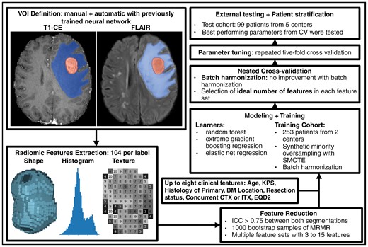
Summarized overview of our workflow. After manual and automatic definition of the volume of interest (VOI), we extracted 104 original features from each metastasis and edema segmentation. We reduced the number of features in each set with MRMR. Furthermore, we added up to 8 clinical features and combined all features into multiple different feature sets. The optimal number of features in each set was determined with a nested cross-validation. The optimal parameters for our selected learners were chosen based on a 5-fold cross-validation. The best parameters for each learner-feature-combination were tested in the external test cohort.
Baseline Clinical Models
To create a baseline for comparison with our radiomic models, we first tested the predictive value of 2 established clinical indices with univariate Cox analysis: The recursive partitioning analysis48 and the Graded Prognostic Assessment (GPA)49 index. They reached a CI of 0.47 and 0.52 in the internal validation, respectively. In external testing, recursive partitioning analysis again performed worse with a CI of 0.39 compared to GPA with a CI of 0.44. We also tested the most recent disease-specific GPA (dsGPA)50 available at the time of data collection. Due to missing information or histologies not covered by this version of the dsGPA, we had a reduced training and test cohort of 200 and 71 patients, respectively. Univariate Cox analysis yielded a CI of 0.44 and 0.46 for internal validation and external testing, respectively.
Model Performance
The performances in the internal validation, as well as in the multicentric external test cohort, are shown in Table 2. To determine the best overall learner, we ranked the performance across all feature sets and found that ENR ranked best, followed by RF and xgboost with mean ranks of 1.4, 1.6, and 2.9, respectively. Therefore, all further experiments were conducted with ENR. For completeness, the results obtained by RF and xgboost are shown in Supplementary Tables 9 and 10. The highest mean CI across all 5 folds and 10 iterations of the cross-validation was achieved with the comb + pre-OP feature set (CI = 0.67).
Performance in Internal Validation and External Testing
| Group | Learner | pre-OP | pre-OP + BMV | Post-OP | RT | T1-CE | FLAIR | comb | comb + pre-OP | comb + pre-OP + BMV |
|---|---|---|---|---|---|---|---|---|---|---|
| 5-fold CV | ENR | 0.64 | 0.63 | 0.63 | 0.63 | 0.65 | 0.47 | 0.62 | 0.67 | 0.67 |
| RF | 0.63 | 0.63 | 0.63 | 0.63 | 0.61 | 0.58 | 0.64 | 0.66 | 0.66 | |
| xgboost | 0.54 | 0.56 | 0.53 | 0.56 | 0.58 | 0.55 | 0.62 | 0.65 | 0.64 | |
| external test cohort | ENR | 0.70 (0.53–0.83) | 0.70 (0.54–0.83) | 0.65 (0.51–0.82) | 0.70 (0.56–0.83) | 0.76 (0.63–0.84) | 0.50 (NA–NA) | 0.69 (0.55–0.80) | 0.77 (0.61–0.87) | 0.72 (0.57–0.82) |
Parameter tuning and internal validation were performed with 10 iterations of a 5-fold cross-validation. The mean performance over all folds and iterations is given. The 95% confidence intervals within the test set (in parenthesis) are based on 10 000 bootstrap samples. The combination of ENR learner and comb + pre-OP feature set performed best with a mean CI of 0.67 (in bold). Adding BMV did not improve performance. By ranking the performance of the models across all feature sets, we identified ENR as the best learner and, therefore, tested this learner on the external test cohort. Again, the best performance was seen with the comb + pre-OP feature set (CI = 0.77, in bold).
The comb + pre-OP feature set also led to the highest performance in the external test cohort and achieved a CI of 0.77. While the T1-CE feature set achieved a CI of 0.76, FLAIR was only able to reach 0.50. The 3 clinical feature sets performed slightly worse than our radiomic feature sets or the combined feature sets: The pre-OP, post-OP, and RT feature sets reached a CI of 0.64, 0.63, and 0.63 in the internal validation, respectively. In external testing, they achieved a CI of 0.70, 0.65, and 0.70, respectively. While adding the BMV to the pre-OP feature set did not change the predictive performance, adding it to comb + pre-OP led to worse results with a CI of 0.72.
For reproducibility, we list the beta values used by our best model (comb + pre-OP ENR) in Supplementary Table 11. The corresponding calibration curve to this model is shown in Figure 3 (right panel). Furthermore, we calculated the time-dependent area under the receiver operating characteristic curve (AUC) by transforming the continuous risk rank to an event probability distribution. The proposed model reached a mean of 0.80. Supplementary Figure 2 shows the plotted time-dependent AUC.
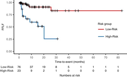
Kaplan–Meier analysis. We created dichotomous predictions of the comb + pre-OP ENR model by using the 66th percentiles of the continuous risk ranks in the training cohort as cutoffs for patient stratification. There were 6 and 10 events in the low-risk group of 76 patients and the high-risk group of 23 patients, respectively. We found a significant difference in freedom from local failure (FFLF) between the predicted low- and high-risk groups (P < .001) in the multicenter external test cohort. After 24 months, we found a FFLF of 91% and 26% in the groups, respectively.
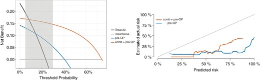
Decision curve analysis (left) and calibration curve (right). Using the same groups as in Figure 2, we found a net benefit of our predictive model compared to treating all patients in the relevant threshold range from 5% to 30% through decision curve analysis (left). A decision model shows a clinical benefit if the respective curve shows larger net benefit values than reference strategies. The combination of radiomic features derived from T1-CE, FLAIR, and pre-OP features (comb + pre-OP) resulted in a higher net benefit compared to using only the clinical pre-OP features and treating all patients or none. The calibration curve on the right was created by transforming the continuous risk rank predicted by the best comb + pre-OP ENR model (in orange) and by the clinical pre-OP ENR model (in blue) to event probabilities at 24 months. Although both models seem to overestimate the actual risk of our patients, the comb + pre-OP model predicted the risk closer to the actual risk.
Patient Stratification
Using the cutoffs determined by the training cohort as described above, our comb + pre-OP ENR model was able to significantly stratify the patients into 3 risk groups with a low, medium, and high risk of LF (P = .0001, Chi-squared Test). A Kaplan–Meier analysis with all 3 groups is shown in Supplementary Figure 3.
By combining the low- and medium-risk groups into one, we created dichotomous predictions. Kaplan–Meier analysis (Figure 2) illustrates the survival in each risk group. Decision curve analysis using these predictions showed a net benefit of our predictive model compared to treating all patients in the relevant threshold range (Figure 3).
The Relevance of Brain Metastasis Volume
The predictions of our comb + pre-OP ENR model did weakly correlate with the cumulative BMV or BMV of the largest BM (Spearman’s rank correlation: r = 0.246 (P = .014) and 0.254 (P = .011), respectively).
While cumulative BMV alone was highly predictive in the test cohort, with a CI of 0.76 in a univariate Cox analysis, it only achieved a CI of 0.53 in internal validation. Using the BMV of only the largest BM increased the internal validation and external testing performance to 0.55 and 0.77, respectively. There was no significant difference in the BMV between the training and test cohort (P = .64, Wilcoxon rank sum test).
Stratifying our test set into small and large BMs by dividing the set at the median cumulative volume (12.6 millimeter³) resulted in groups with 4 and 12 events, respectively. Our best model scored a CI of 0.58 and 0.78 in the respective groups. The model significantly risk-stratified the patients in the large BMV group, but not in the small BMV group (corresponding Kaplan–Meier analysis are depicted in Supplementary Figures 4 and 5).
When repeating the feature reduction, parameter tuning, training, and testing with the radiomic features extracted only from the largest BM, the ENR learner was able to reach a CI of 0.75 (comb + pre-OP + BMV, Table 3). The previously best feature set (comb + pre-OP) only achieved a performance of 0.70. The selected radiomic features are listed in Supplementary Table 4.
Performance in the Test Set With Automated U-Net Segmentations and Segmentations of only the Largest Metastasis
| Group | Learner | T1-CE | FLAIR | comb | comb + pre-OP | comb + pre-OP + BMV |
|---|---|---|---|---|---|---|
| Manual segmentation | ENR | 0.76 (0.63–0.84) | 0.50 (NA–NA) | 0.69 (0.55–0.80) | 0.77 (0.61–0.87) | 0.72 (0.57–0.82) |
| Largest BM | ENR | 0.72 (0.59–0.82) | 0.50 (NA–NA) | 0.63 (0.54–0.79) | 0.70 (0.58–0.86) | 0.75 (0.57–0.84) |
| U-net segmentation | ENR | 0.58 (0.41–0.75) | 0.46 (0.31–0.64) | 0.58 (0.41–0.75) | 0.72 (0.55–0.83) | 0.69 (0.53–0.80) |
In addition to using our manual segmentations, we also trained and tested our proposed model on segmentations of only the largest BM and automatically generated U-Net segmentations. Since the clinical feature sets are independent of the segmentation method, they were not added to this analysis. Compared to the manual segmentations, the results were, on average 0.08 and 0.03 points worse, respectively. The best performance is printed in bold.
End-to-End Model Using Neural Network-Based Automatic Segmentations
The neural network-based segmentations had a median DSC of 0.94 (IQR: 0.92–0.96) and 0.92 (0.87–0.95) in comparison to the manual segmentation for the metastasis and edema labels, respectively. The mean DSC was slightly lower at 0.92 (95% confidence interval: 0.92–0.93) and 0.89 (95% confidence interval: 0.88–0.90), respectively.
To test the predictive value of neural network-based segmentations and therefore test the feasibility of a fully automated workflow, we repeated all steps, starting with the feature reduction, followed by an additional parameter tuning and training run with radiomic features extracted from the automatic created segmentations. The selected features are listed in Supplementary Table 5. The results for our ENR learner are shown in Table 3. The best test results with this data were again obtained with the comb + pre-OP feature set (CI = 0.72). Overall, we observed an average decrease in performance by 0.08.
Impact of N4 Bias Field Correction
To test the possible influence of MR intensity inhomogeneities,51 we extracted the radiomic features again after applying N4 bias field correction.52 Repeating our workflow with these features resulted in minor changes. The selected features are listed in Supplementary Table 6. Comb + pre-OP + BMV performed best with these features, reaching a CI of 0.77. The previously best feature set (comb + pre-OP) performed slightly worse, reaching a CI of 0.76.
Predictive Performance of the Delivered Radiation Dose
Recent studies3 suggest that a higher delivered radiation dose may improve local control in BMs. Since dose information is completely independent of radiomic features, we wanted to test the prognostic value of radiation dose in the form of EQD2 alone and in combination with our combined feature set with univariate Cox analysis and our established pipeline, respectively. In univariate Cox analysis, EQD2 alone resulted in a CI of 0.54 and 0.60 in internal validation and external testing. The combination of EQD2 and the combined feature set yielded a CI of 0.60 and 0.70 in internal validation and external testing with the ENR learner.
Discussion
In this work, we were able to develop radiomics-based machine learning models that were able to predict FFLF better than clinical features alone. Our best model was trained with a combination of radiomic and clinical features and achieved a CI of 0.77 in a multicenter external test cohort outperforming any clinical predictive model. Our final model’s predictions significantly stratified the test patients into 2 risk groups and achieved an incremental net clinical benefit.
When using automatically generated segmentations from a previously trained neural network, the models performed slightly worse, with an average performance loss of 0.08. While the neural network-based segmentations were of good quality with a median DSC of 0.94 for the metastasis label, the slightly lower mean DSC shows some outliers. This is also shown by the 5th and 10th percentile of the metastasis label of 0.79 and 0.88. Removing the segmentations with a DSC lower than the 10th percentile in the respective sets (training set: DSC < 0.88, test set: DSC < 0.86) led to improved prediction results only worse by an average CI of 0.02 compared to the manual segmentation. The comb + pre-OP ENR model was able to reach a respectable CI of 0.72 in external testing with the automatically generated segmentations, which improved to 0.77 after removing the outliers. This demonstrates that with sufficient segmentation quality, an end-to-end solution is possible without clinician intervention.
While the inclusion of the N4 bias field correction resulted in different feature selections (Supplementary Table 6), it did not improve performance. Because it would add another step to our preprocessing pipeline, we decided not to include the bias field correction. In this way, we can achieve a simpler applicability of our models.
The results in the external test cohort were, on average, better by a CI of 0.04. This may be explained by the larger amount of data available for training: The models tested on the external cohort were trained on all training data, while for internal validation, only 80% of the data was used for training, while testing was performed on the remaining 20%.
Patients at high predicted risk for LF may benefit from risk-adapted therapy and follow-up. This may include dose escalation of SRT or the use of wider CTV margins, which have been shown to improve local control.53 In addition, therapy may be supplemented with systemic agents that cross the blood-brain barrier. Finally, more frequent follow-up may help in the early detection of potential LF.
Several studies have approached predicting the LF of BMs. Most of them interpreted the prediction as a classification task and therefore only predicted whether an event occurred at a predetermined time.16–18,54–63 In contrast, we approached the task as a survival task and therefore predicted a combination of event and time in terms of FFLF.
Another study predicting the event and time of LF by Huang et al.64 used Cox proportional hazards models and found that non-small cell lung cancer BMs with a higher zone percentage were more likely to respond favorably to Gamma Knife radiosurgery. In contrast to the treatment with surgery and adjuvant SRT in our study, the aforementioned studies focused on BMs treated with SRT, WBRT, and immune checkpoint inhibitors. Only one monocentric study with 67 patients by Mulford et al.57 investigated the prediction of local recurrence after surgical resection and adjuvant stereotactic radiosurgery, and found that radiomic features provided more robust predictive models of local control rates than clinical features (AUC = 0.73 vs. 0.40). Unlike our study, they predicted LF as a binary classification task.
Another unique feature of our study is the multicenter external test cohort with patients treated at 5 different centers in multiple countries. In contrast to our study, the aforementioned studies all tested their models on an internal validation set and were therefore not tested on such a wide variety of scanners and imaging protocols as our models were.
Contrary to findings in previous studies,65 the cumulative BMV and the BMV of the largest BM were not predictive in the internal validation, where they only reached a CI of 0.53 and 0.55, respectively. Since outcome and BMV appear to be independent in the training cohort, radiomic features representing BM size were not selected by our feature reduction algorithm. The only selected shape class feature in the best-performing feature set was metastasis flatness. Moreover, there was only a minor correlation (r = 0.25) between the predictions of the radiomic model and BMV. This shows that radiomics can predict LF based on features that do not directly represent BM size or volume.
Compared to approaches focusing on the use of neural networks, the use of classical machine learning has some advantages: Because only a small number of features are fed into the model, it becomes more comprehensible. Since it is known how the radiomics features are computed, it is possible to infer the clinical correlates. As a test, we compared the 5 patients with the highest and lowest rank to find visual differences in imaging. The results alongside some example images are shown in Supplementary Figure 6. Neural networks, on the other hand, are more intransparent black boxes, and it is difficult to understand exactly which characteristics of the tumor are predictive. In addition, neural networks often require the use of a graphics processing unit to complete predictions in a reasonable amount of time, while our models run on the central processing unit (CPU) and can, therefore, run on low-end hardware.
Nevertheless, this work has several limitations: Training the models with only a limited number of features extracted from the segmentations prevents them from taking other factors into account, such as the surrounding tissue. Furthermore, segmentations of consistent quality are necessary for reliable results. In this study, all segmentations were created by the same person. To reduce the influence of the personal segmentation style, only features with a high correlation between manual and automatic segmentations were used for further modeling. The sole use of automatically generated segmentations may help with this limitation.
In daily clinical practice, it is a difficult task to differentiate LF from radiation necrosis or pseudoprogression.66 Although board-certified radiologists made the diagnosis, some cases may have been misclassified, which is unavoidable in such studies.
Around one-quarter of our patients had multiple BMs. By using the cumulative BMV as a feature, we not only took the volume of the resected BM into account but also the volume of all additional BMs. In our additional analysis, we used the largest metastasis as a surrogate for the resected metastasis. The largest metastasis accounted for a median of 90% (IQR: 75%–98%) of the total tumor burden in patients with multiple metastases. Because the smaller metastases represented only a small proportion of the total tumor burden, we considered the largest metastasis as the resected metastasis with reasonable certainty. When using the radiomic features extracted from the largest metastasis, the mean across all models decreased by 0.03 compared to using the combined segmentation of all BMs. From this, we can conclude that segmenting all BMs did not harm the prediction of LF of the resected BM.
In addition, radiomic features were extracted from a total of 12 synthesized T2-FLAIR sequences (6 in the training cohort and 6 in the test cohort). Excluding these patients from the training and test sets resulted in a slight increase in performance. The largest increase in performance was found in the combined feature set (CI = 0.72 from 0.69). Furthermore, the T1-CE model showed the second-largest increase in performance, surpassing our previous best feature set (comb + pre-OP), which showed no change in performance. Since the new best model did not even include features extracted from the T2-FLAIR sequence, we can conclude that radiomic features extracted from the synthesized T2-FLAIR sequences did not noticeably affect the performance of our model and the increase in performance may be attributed to the exclusion of difficult cases.
Despite these limitations, we were able to develop a model to predict FFLF of BMs after resection and adjuvant SRT. The model performed well in a multicenter external test cohort with a variety of MRI scanners and imaging and therapy protocols. This model may help to tailor treatment to a patient’s individual risk of metastasis recurrence, thereby improving the overall management of BMs. We have published the model as an easy-to-use web app (https://radonc-ai.shinyapps.io/Radiomics_App/), where the user can either upload the required MRI sequences and segmentations or input previously extracted radiomic features.
Supplementary material
Supplementary material is available online at Neuro-Oncology (https://dbpia.nl.go.kr/neuro-oncology).
Funding
This work was funded by the Deutsche Forschungsgemeinschaft (DFG, German Research Foundation, Project number 504320104—PE 3303/1-1 (JCP), WI 4936/4-1 (BW), RU 1738/5-1 (DR)).
Conflict of interest statement
T.B.B.: Honoraria: Merck, Takeda, Dalichi Sankyo.
A.W.: Grants: EFRE, Siemens; Consulting fees: Gilead, Hologic Medicor GmbH; Honoraria: Accuracy, Universitätsklinikum Leipzig AöR, Sanofi-Aventis GmbH; Travel support: DKFZ, DEGRO; Board: IKF GmbH (Krankenhaus Nordwest).
Cl.Z.: Co-editor on the advisory board of “Clinical Neuroradiology,” Leadership: President of the German society of Neuroradiology (DGNR)
Be. M.: Grants: BrainLab, Zeiss, Ulrich, Spineart; Royalities: Medacta, Spineart; Consulting fees and Honoraria: Medacta, Brainlab, Zeiss; Travel support: Brainlab, Medacta; Stock: Sonovum.
M.G.: Grants: Varian/Siemens Healthineers, AstraZeneca, ViewRay Inc.; Honoraria: AstraZeneca; Leadership: ESTRO president elect, SAMO board member.
N.A.: Grants: ViewRay Inc., AstraZeneca, SNF, SKL, University CRPP; Consulting Fees: ViewRay Inc., AstraZeneca; Honoraria: ViewRay Inc., AstraZeneca; Travel support: ViewRay Inc., AstraZeneca; Safety monitoring/advisory board: AstraZeneca, Equipment: ViewRay Inc.
R.A.E.S.: Grants: Accuray; Consulting Fees: Novocure, Merck, AstraZeneca; Honoraria: Accuray, AstraZeneca, BMS, Novocure, Merck, Takeda; Travel support: Merck, Accuray, AstraZeneca; Safety monitoring/advisory board: Novocure, Merck; Stock: Novocure.
J.D.: Grants: RaySearch Laboratories AB, Vision RT Limited, Merck Serono GmbH, Siemens Healthcare GmbH, PTW-Freiburg Dr. Pychlau GmbH, Accuray Incorporated; Leadership: CEO at HIT, Board of directors at University Hospital Heidelberg; Equipment: IntraOP.
O.B.: Grants: STOPSTORM.eu; Leadership: Board member of the working groups for Stereotactic Radiotherapy of the German Radiation Oncology and Medical Physics Societies, Section Editor of “Strahlentherapie und Onkologie.”
K.F.: Grants: Master of Disaster (Gyn Congress, Essen, Germany).
S.E.C.: Grants, Consulting fees and Honoraria: Roche, AstraZeneca, Medac, Dr. Sennewald Medizintechnik, Elekta, Accuray, B.M.S., Brainlab, Daiichi Sankyo, Icotec AG, Carl Zeiss Meditec AG, HMG Systems Engineering, Janssen; Safety monitoring/advisory board: CureVac DSMB Member; Leadership: NOA Board Member, DEGRO Board Member.
D.R.: Grants: DFG, ERC, EPSRC, BMBF, Alexander von Humboldt Stiftung; Consulting fees: ERC.
B.W.: Grants: DFG, NIH, Deutsche Krebshilfe, BMWi; Consulting fees and Stock: Need; Honoraria: Philips, Novartis.
J.C.P.: Honoraria: AstraZeneca, Support for current manuscript: German Research Foundation. The remaining authors have no potential conflicts of interest to disclose.
Authorship statement
All authors were involved in the data curation and acquisition of resources. Formal analysis, methodology, and software: J.A.B. and J.C.P. Visualization: J.A.B.. Writing—Original Draft: J.A.B., F.K., B.W., and J.C.P.. Writing—Review & Editing: J.A.B., F.K., S.M.C., T.B.B., A.W., Be.M., S.R., O.R., O.B., Co.Z., A.B.Z., A.L.G., B.W., and J.C.P..Supervision: M.P., S.E.C., B.W., and J.C.P.. Project administration: K.A.E., S.E.C., D.B., and J.C.P.. Funding acquisition: S.E.C., R.U., B.W., and J.C.P.. All authors approved the manuscript.
Data availability
The trained model is available as a shiny web app. Sharing of imaging and tabular features was not possible due to institutional review board constraints and data protection rights in the retrospective, multicenter setting.


