


Abstract
Background. During the follow-up in a randomized controlled trial (RCT), participants may receive additional (non-randomly allocated) treatment that affects the outcome. Typically such additional treatment is not taken into account in evaluation of the results. Two pivotal trials of the effects of hemodiafiltration (HDF) versus hemodialysis (HD) on mortality in patients with end-stage renal disease reported differing results. We set out to evaluate to what extent methods to take other treatments (i.e. renal transplantation) into account may explain the difference in findings between RCTs. This is illustrated using a clinical example of two RCTs estimating the effect of HDF versus HD on mortality.
Methods. Using individual patient data from the Estudio de Supervivencia de Hemodiafiltración On-Line (ESHOL; n = 902) and The Dutch CONvective TRAnsport STudy (CONTRAST; n = 714) trials, five methods for estimating the effect of HDF versus HD on all-cause mortality were compared: intention-to-treat (ITT) analysis (i.e. not taking renal transplantation into account), per protocol exclusion (PPexcl; exclusion of patients who receive transplantation), PPcens (censoring patients at the time of transplantation), transplantation-adjusted (TA) analysis and an extension of the TA analysis (TAext) with additional adjustment for variables related to both the risk of receiving a transplant and the risk of an outcome (transplantation–outcome confounders). Cox proportional hazards models were applied.
Results. Unadjusted ITT analysis of all-cause mortality led to differing results between CONTRAST and ESHOL: hazard ratio (HR) 0.95 (95% CI 0.75–1.20) and HR 0.76 (95% CI 0.59–0.97), respectively; difference between 5 and 24% risk reductions. Similar differences between the two trials were observed for the other unadjusted analytical methods (PPcens, PPexcl, TA) The HRs of HDF versus HD treatment became more similar after adding transplantation as a time-varying covariate and including transplantation–outcome confounders: HR 0.89 (95% CI 0.69–1.13) in CONTRAST and HR 0.80 (95% CI 0.62–1.02) in ESHOL.
Conclusions. The apparent differences in estimated treatment effects between two dialysis trials were to a large extent attributable to differences in applied methodology for taking renal transplantation into account in their final analyses. Our results exemplify the necessity of careful consideration of the treatment effect of interest when estimating the therapeutic effect in RCTs in which participants may receive additional treatments.
INTRODUCTION
The randomized controlled trial (RCT) is the preferred design to assess the effects of medical treatments. When patients switch to the other trial treatment arm, receive additional treatment that is not randomly allocated or stop their treatment, estimation of treatment effects may not be straightforward, notably when treatment switching depends on patient characteristics [1].
In RCTs comparing hemodiafiltration (HDF) with hemodialysis (HD) on the risk of mortality among patients with end-stage renal disease (ESRD), during follow-up a subset of patients may receive another (non-randomly allocated) treatment that effectively improves patient outcome. For example, renal transplantation is highly effective in reducing mortality risk in ESRD patients and differences in handling renal transplantation during follow-up in the analysis of a trial may lead to different results [2]. Two pivotal dialysis trials reported conflicting findings: results of the Estudio de Supervivencia de Hemodiafiltración On-Line (ESHOL) trial indicated improved survival for HDF compared with HD {all-cause mortality hazard ratio [HR] 0.70 [95% confidence inaterval (CI) 0.53–0.92]}, while results from The Dutch CONvective TRAnsport STudy (CONTRAST) analysis reported no difference in mortality between treatment groups [HR 0.95 (95% CI 0.75–1.20] [3, 4]. These differing results may be explained by a number of differences between the trials. Notably, in the original ESHOL study, patients were censored at the time of renal transplantation, so no patient information on all-cause mortality was collected after renal transplantation [4]. Such loss to follow-up may introduce bias if censoring is associated with the allocated treatment and the risk of the outcome [1, 5]. Alternatively, in the CONTRAST trial, participants were followed-up for the primary outcome (i.e. all-cause mortality), irrespective of a renal transplant and the effects of the dialysis treatments were estimated based on an intention-to-treat (ITT) analysis (and ignoring transplantation) [3]. Furthermore, none of the trial analyses took renal transplantation into account.
Post-randomization renal transplantation may induce differences in patient characteristics between treatment groups in dialysis trials since the probability of receiving a renal transplant may not only depend on patient characteristics, but also on the randomly allocated treatment a patient receives (here, on the dialysis modality). For example, patients treated with HDF may more often receive a renal transplant compared with patients treated with HD. As a result, in dialysis trials, the probability of receiving a transplant may differ between treatment arms. Therefore, restricting the analysis to those who did not undergo a renal transplant (e.g. in a per protocol analysis) may result in incomparable treatment groups. As an example, assume that 20% of HDF-treated patients receive a renal transplant compared with 10% of HD-treated patients and that transplant is more likely in younger patients. Due to the randomization procedure, the age distribution at baseline of patients receiving HDF or HD is comparable. However, restricting the analysis to those patients who did not undergo a renal transplant leads to excluding a larger proportion (20%) of patients (who are, on average, younger) in the HDF treatment group compared with the 10% of patients in the HD treatment group. The remaining patients in the HDF treatment group are, on average, older than the patients in the HD treatment group, a situation referred to as confounding, because age is now associated with treatment as well as the outcome (here, survival).
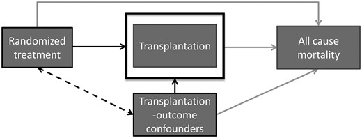
Causal diagram of renal transplantation in RCTs of dialysis modalities. When treatment is related to receiving a transplant and patient characteristics (transplantation–outcome confounders) are related to both transplantation as well as experiencing the outcome, selection bias arises when only patients who did not receive a transplant are selected for analysis (or similarly, when we condition on or adjust for transplantation). Since patient characteristics for patients receiving a transplant are different from those who do not receive a transplant and a different proportion of patients in each treatment group receives a transplantation, the remaining treatment groups are no longer comparable on these transplantation–outcome confounders. The induced bias is a result of selection of patients for analysis (i.e. non-transplanted patients), which is different between treatment groups (i.e. patients in the treatment group are more likely to receive transplantation), and is therefore called selection bias. Depending on the method of analysis, this may bias the estimated treatment effect.
When the mechanism of allocating transplant kidneys differs between studies, this may contribute to differences in effect estimates between studies, depending on the applied method of analysis. To study the value of taking competing risks into account when evaluating therapy effect, we set out to determine to what extent approaches that take competing risks (i.e., renal transplantation) into account may explain the conflicting findings between these two trials.
MATERIALS AND METHODS
Data design and study population
Individual patient data from the CONTRAST and ESHOL studies were used for the current study. Detailed descriptions of the study designs, patient characteristics and treatment procedures of each of the studies have been reported elsewhere [3, 4, 7, 8]. In the ESHOL study, patients who received a renal transplant had been censored alive in the previously published analyses, an approach potentially leading to bias. The ESHOL dataset was completed by adding follow-up data on all-cause mortality for those patients who had discontinued randomized treatment (received a renal transplant), as described previously [7, 9]. The ESHOL study included 906 patients; 456 were randomized to receive HDF and 450 to HD. The median follow-up time was 3 years (range 0.01–3.08) [4]. The CONTRAST study included 714 patients; 358 received HDF and 356 were allocated to HD. The median follow-up time was 2.90 years (range 0.04–6.56) [3]. Due to missing outcome and time of transplantation data, four patients were excluded from the current analysis of the ESHOL dataset.
Given a large sample size, randomization is expected to create treatment groups that are on average comparable with respect to patient characteristics, that is, treatment is independent of patient characteristics. Receiving a renal transplant, however, may be dependent on patient characteristics. For example, younger patients with less comorbidity are more likely to receive a renal transplant. These patient characteristics are also predictive of the outcome (all-cause mortality). Since these patient characteristics are related to both transplantation and the outcome, we will refer to them as confounders of the transplantation–outcome relation (see Figure 1).
While randomization is expected to achieve equal distributions of patient characteristics between treatment arms, in reality differences in patient characteristics may actually be present. Adjustment for variables related to the outcome will remove any remaining confounding by observed variables and tends to improve power in all mentioned methods of analysis [10].
Methods to analyse dialysis trials in the presence of renal transplantation
We compared five methods to handle renal transplantation in dialysis trials. These methods are described in more detail below and summarized in Table 1.
Methods to deal with transplantation during follow-up (competing treatment) in randomized trials of haemodialysis
| Method | Description | Interpretation of effect estimate | Potential for bias |
|---|---|---|---|
| Intention-to-treat (ITT) | Data from all patients is used. Treatment status is analysed as allocated. Transplantation is ignored in the analysis | The effect of treatment in settings with rates and allocation mechanisms of transplantation similar to the current trial | Unbiased when randomization is successful |
| Per protocol exclusion (PPexcl) | Exclude patients who receive transplantation from the analysis | The effect of treatment in the group that completes the trial according to protocol (i.e. patients who do not receive transplantation); in other words, the effect of treatment in non-transplanted patients | This effect is biased when both treatment affects the probability to receive transplant and transplantation–outcome confounders are present. Bias can be avoided by adjusting for transplantation–outcome confounders |
| Per protocol censored (PPcens) | Censor patients who receive transplantation at transplantation (follow-up information after transplantation is discarded) | See per protocol exclusion. Difference is that we gain the patient time until transplantation for patients receiving transplantation. This may lead to narrower confidence intervals | See per protocol exclusion |
| Accounting for transplant as time-dependent covariate (TA) | Transplantation is added to the outcome model as a time-dependent covariate | The effect of treatment in transplanted and non-transplanted patients | This effect is biased when treatment affects the probability to receive transplant and there are transplantation–outcome confounders. Bias can be avoided by adjusting for transplantation–outcome confounders |
| Accounting for transplant as time-dependent covariate and adjustment for transplantation–outcome confounders (TAext) | Transplantation is added to the outcome model as a time-dependent covariate. Additionally, confounders of the transplantation–outcome relationship are included in the model for the outcome | The effect of treatment in transplanted and non-transplanted patients | This effect is biased when important transplantation–outcome confounders are unmeasured or unknown and therefore cannot be adjusted for |
In RCTs comparing HDF with HD on the risk of mortality among patients with ESRD, during follow-up a subset of patients may receive a non-randomly allocated competing treatment (i.e. a renal transplantation) that effectively improves patient outcome.
ITT analysis
In ITT analysis, patients are analysed according to the treatment group they are allocated to. This analysis ignores the fact that a subgroup of patients received a renal transplantation and stopped the allocated treatment. We are not taking into account other forms of treatment switching (e.g. from HD to HDF or the other way around). Since the equal distributions of patient characteristics (including those also associated with the outcome) between treatment groups obtained by randomization remains intact, ITT analysis allows for unbiased effect estimation. The ITT estimate is interpreted as the effect of the treatment ‘strategy’, implying that renal transplantation during the follow-up period of the trial is an inherent part of the treatment strategy. In other words, results from the current study will not be applicable to a future population in which the proportion of patients receiving a renal transplant and/or the patient characteristics of those receiving a transplant (i.e. the ‘strategies’) differ from those in the current trial. ITT effects are sometimes called pragmatic or ‘total effects’, since the ITT estimate includes the effect treatment has through changing the probability of receiving additional interventions (including a renal transplant) after the treatment has been initiated.
Per protocol (PP) exclusion analysis
Similar to ITT analysis, in PP analysis, patients are analysed according to the treatment group they were allocated to. However, in per protocol exclusion (PPexcl) analysis, those subjects who stop receiving their allocated treatment after receiving a renal transplant are excluded from the analysis. The PP estimate is interpreted as the effect of treatment in the subset of patients that complete the trial according to the protocol (here, non-transplanted patients). Besides the fact that renal transplantation improves survival, patients receiving renal transplantation have a different prognosis (e.g. these patients are on average younger) compared with patients who remain on treatment, therefore PP analyses are biased in case transplantation occurs more often in one of the treatment groups [1, 11]. However, when these prognostic differences (i.e. confounders of the transplantation–outcome relation) are adjusted for, the estimated treatment effect should be unbiased, provided no other sources of bias exist [1].
PP censoring analysis
In a per protocol censoring (PPcens) analysis, patients receiving a renal transplant are not excluded from the analysis (as in the PPexcl analysis), but are censored (i.e. considered excluded without developing the outcome) at the time they receive the transplant. Similar to PPexcl, PPcens analyses are biased in case transplantation occurs more often in one of the treatment groups, and the reasons for this are associated with the outcome. However, the bias is less pronounced compared with PPexcl, since patient time until transplantation is still accounted for in the analysis. Again, adjustment for confounding leads to an unbiased effect estimate, provided no other sources of bias exist.
Including transplantation in the outcome model, transplantation-adjusted (TA) analysis
Treatment effects obtained by ITT and PP may be of limited generalizability. Specifically, PP effects are only applicable to patients who do not receive transplantation, and ITT effects are only generalizable to populations with a comparable percentage and allocation mechanism of transplantation. Therefore it may be of interest to estimate the ‘controlled direct effect’ of treatment, which is the effect of treatment (i.e. dialysis) excluding the effect treatment has through changing the probability of receiving a renal transplant (either by chance or through some causal known or unknown mechanism) [12]. The controlled direct effect of treatment assumes the same effect of treatment in patients receiving transplantation as well as non-transplanted patients [13]. The controlled direct effect is estimated by including transplantation in the outcome model. The TA estimates can be interpreted as the biological effect of treatment on the outcome, independent of the effect of treatment on the probability of a transplant. Transplantation should be modelled as a time-dependent covariate in the outcome model [14, 15].
TA analysis adjusted for transplantation–outcome confounders
Since TA effect estimates are conditional on transplantation, the resulting effect estimates are prone to bias (as in the PP analysis). Therefore, it is necessary to adjust for transplantation–outcome confounders in the outcome model. The extension of the TA analysis (TAext) effect may be biased if important confounders for the relationship between transplantation and the outcome are unmeasured or when observed confounders are not assessed correctly. In our analyses we adjusted for measured confounders, including age, history of cardiovascular disease, serum creatinine, diabetes mellitus, haemoglobin, albumin, body surface area, months on dialysis and C-reactive protein.
Statistical analysis
R version 3.0.1 (www.r-project.org) was used to perform the statistical analyses [16]. Before applying the five methods of analysis described above, missing data on transplantation–outcome confounders were imputed using multiple imputation by chained equations using the R package ‘mice’ [17]. Log transformations of months of dialysis and C-reactive protein were taken to comply with the assumption of normality, which is necessary for multiple imputation. A total of 10 imputed datasets were created for each study. The R package ‘survival’ was used to fit the Cox proportional hazards (PH) models. Cox PH models were applied. When transplantation was included in the Cox PH models, it was included as a time-varying covariate in order to prevent immortal time bias. Immortal time bias is the result of classifying patient time before onset of treatment as time on treatment. Because patients have to survive until they receive the treatment of interest, the misclassified time before the start of treatment is called immortal time and the resulting bias is immortal time bias [14, 15, 18, 19]. Results from the imputed datasets were combined using Rubin’s rule to obtain HRs and 95% CIs [20], for which the function MIcombine from the package “mitools” was used. Log-log and Schoenfeld residual plots were obtained and checks for PH assumptions were performed.
RESULTS
Baseline characteristics of patients enrolled in the ESHOL and CONTRAST studies are presented in Table 2. A total of 28 326 observation-months from 902 patients were included in the analysis of the ESHOL study. The mean age of patients was 65.5 years [standard deviation (SD) 14.3] and 298 (33.0%) had a history of cardiovascular disease. A total of 179 (19.8%) patients received a renal transplant during follow-up; 101 (22.2%) HDF patients were transplanted compared with 78 (17.5%) HD patients. Missing covariate data were most common for C-reactive protein, which had missing entries for 211 (23.4%) patients. The CONTRAST study consisted of 26 398 observation-months from 714 patients. The mean age of patients was 64.1 years (SD 13.7) and 313 (43.8%) had a history of cardiovascular disease. During follow-up, 151 (21.1%) patients received a renal transplant; 78 (21.8%) HDF versus 73 (20.5%) HD patients were transplanted. Again, missing covariate data were most prevalent for C-reactive protein, for which 309 (43.3%) patients had missing entries.
Baseline characteristics of patients in CONTRAST and ESHOL
| CONTRAST | ESHOL | |||||||||||
|---|---|---|---|---|---|---|---|---|---|---|---|---|
| All patients (n = 714) | Transplanted [n = 151 (21.1%)] | Non-transplanted [n = 563 (78.9%)] | All patients (n = 902) | Transplanted [n = 179 (19.8%)] | Non-transplanted [n = 723 (80.2%)] | |||||||
| No. missing values | Overall | HD | HDF | HD | HDF | No. missing values | Overall | HD | HDF | HD | HDF | |
| (n = 73) | (n = 78) | (n = 283) | (n = 280) | (n = 78) | (n = 101) | (n = 368) | (n = 355) | |||||
| Male sex, n (%) | 0 | 445 | 44 | 44 | 187 | 170 | 0 | 602 | 48 | 71 | 237 | 246 |
| (62.3) | (60.3) | (56.4) | (66.1) | (60.7) | (66.7) | (61.5) | (70.3) | (64.4) | (69.3) | |||
| Age, mean (SD) | 0 | 64.1 | 55.9 | 51.1 | 66.1 | 67.7 | 0 | 65.5 | 52.7 | 55.5 | 69.4 | 67.1 |
| (13.7) | (11.4) | (12.8) | (13.1) | (12.0) | (14.3) | (13.0) | (11.6) | (12.8) | (14.0) | |||
| History of cardiovascular disease, n (%) | 0 | 313 | 18 | 15 | 144 | 136 | 0 | 298 | 14 | 20 | 140 | 124 |
| (43.8) | (24.7) | (19.2) | (50.9) | (48.6) | (33.0) | (18.0) | (19.8) | (38.0) | (34.9) | |||
| Serum creatinine (mg/dL), mean (SD) | 3 | 9.74 | 11.15 | 11.12 | 9.63 | 9.09 | 33 | 8.02 | 8.25 | 8.90 | 7.91 | 7.83 |
| (2.90) | (2.62) | (2.65) | (2.82) | (2.87) | (2.38) | (2.32) | (2.43) | (2.39) | (2.33) | |||
| Diabetes mellitus, n (%) | 25 | 177 | 12 | 19 | 71 | 75 | 0 | 226 | 13 | 14 | 108 | 90 |
| (24.8) | (16.2) | (24.4) | (25.2) | (26.8) | (25.0) | (16.7) | (13.9) | (29.3) | (25.4) | |||
| Hemoglobin (g/dL), mean (SD) | 1 | 11.8 | 11.8 | 12 | 11.7 | 11.8 | 2 | 12.0 | 12.1 | 12.4 | 11.9 | 11.9 |
| (1.25) | (0.99) | (1.26) | (1.22) | (1.34) | (1.43) | (1.28) | (1.37) | (1.44) | (1.46) | |||
| Albumin (g/dL), mean (SD) | 9 | 4.04 | 4.17 | 4.10 | 4.03 | 4.00 | 24 | 4.09 | 4.20 | 4.21 | 4.03 | 4.08 |
| (0.39) | (0.43) | (0.29) | (0.38) | (0.40) | (0.43) | (0.44) | (0.43) | (0.44) | (0.42) | |||
| Body surface area (m2), mean (SD) | 0 | 1.85 | 1.87 | 1.83 | 1.87 | 1.84 | 1 | 1.73 | 1.73 | 1.76 | 1.72 | 1.74 |
| (0.21) | (0.20) | (0.21) | (0.20) | (0.23) | (0.19) | (0.18) | (0.18) | (0.19) | (0.19) | |||
| Log (months on dialysis), mean (SD) | 0 | 3.22 | 3.42 | 3.12 | 3.22 | 3.20 | 3 | 3.32 | 3.01 | 3.22 | 3.38 | 3.36 |
| (0.87) | (0.83) | (0.81) | (0.88) | (0.88) | (1.14) | (1.00) | (1.18) | (1.17) | (1.12) | |||
| Log (C-reactive protein), mean (SD) | 309 | 1.70 | 1.52 | 1.43 | 1.71 | 1.82 | 211 | 2.09 | 1.86 | 1.92 | 2.13 | 2.14 |
| (1.06) | (1.02) | (1.03) | (1.05) | (1.12) | (0.92) | (0.93) | (0.91) | (0.90) | (0.96) | |||
Due to the nature of multiple imputation and rounding of numbers, the separate diabetes mellitus categories do not sum to the overall diabetes mellitus count.
As expected, in both ESHOL and CONTRAST, baseline characteristics of patients receiving transplantation during follow-up differed from patients who did not receive a renal transplant (Table 2). In the non-transplanted patient group of the ESHOL study, treatment groups differed with respect to history of cardiovascular disease (HD 38.0%, HDF 34.9%) and diabetes mellitus status (HD 29.3%, HDF 25.4%). In the CONTRAST study, transplantation–outcome confounders were comparable in the two treatment groups. For example, the prevalence of a history of cardiovascular disease (HD 50.9% versus HDF 48.6%) and diabetes mellitus (25.2% HD versus 26.8% HDF) were similar.
Table 3 shows the effect of HDF treatment compared with HD treatment on all-cause mortality when applying different analytical methods in the two studies. In ESHOL, the effect of HDF versus HD treatment was estimated to be HR 0.76 (95% CI 0.59–0.97) for the unadjusted ITT. In CONTRAST, the effect of HDF versus HD treatment was estimated to be HR 0.95 (95% CI 0.75–1.20) for the unadjusted ITT.
Estimates of the HR of HDF versus HD for all-cause mortality for different methods in two RCTs: ESHOL and CONTRAST
| ESHOL | CONTRAST | |
|---|---|---|
| Method | HR (95% CI) | HR (95% CI) |
| Intention-to-treat (ITT) | 0.76 (0.59–0.97) | 0.95 (0.75–1.20)a |
| Per protocol censored (PPcens) | 0.73 (0.56–0.94)a | 0.88 (0.69–1.13) |
| Per protocol exclusion (PPexcl) | 0.74 (0.58–0.96) | 0.90 (0.70–1.16) |
| Accounting for transplant as a time-dependent covariate (TA) | 0.77 (0.60–0.99) | 0.95 (0.75–1.21) |
| Accounting for transplant as a time-dependent covariate and adjustment for transplantation–outcome confounders (TAext) | 0.80 (0.62–1.02) | 0.89 (0.69–1.13) |
Original ESHOL and CONTRAST analyses. For the current analyses, the ESHOL dataset was completed by adding follow-up data on all-cause mortality for those patients who had discontinued randomized treatment (received a renal transplant) and were considered alive in the previously published analyses. In the current analysis, four subjects were excluded due to missing data.
Unadjusted PP analysis of the ESHOL study resulted in HR 0.73 (95% CI 0.56–0.94) and HR 0.74 (95% CI, 0.58–0.96) for censoring (PPcens) and exclusion (PPexcl), respectively. In the CONTRAST study, the unadjusted PP analyses resulted in HR 0.88 (95% CI 0.69–1.13) and HR 0.90 (95% CI, 0.70–1.16) for PPcens and PPexcl, respectively.
In ESHOL, TA analysis resulted in HR 0.77 (95% CI 0.60–0.99), while TA analysis in the CONTRAST study resulted in HR 0.95 (95% CI 0.75–1.21). In ESHOL, TA analysis with adjustment for transplantation–outcome confounders (TAext) resulted in HR 0.80 (95% CI 0.62–1.02), while the same analysis in the CONTRAST study resulted in HR 0.89 (95% CI 0.69–1.13).
DISCUSSION
This study assessed whether differences in published effect estimates observed between two RCTs (ESHOL and CONTRAST) investigating the effect of HDF versus HD on mortality in end-stage renal disease could be attributed to the fact that these RCTs applied different methods of analysing the occurrence of renal transplantation during the trial. Indeed, the differences in effects between the two studies attenuated when the same analysis was performed; in particular, adjustment for transplantation–outcome confounders led to more similar effect estimates between the ESHOL and CONTRAST trials. This indicates that differences in applied analytical methods explain part of the differences in effects observed between these trials. Our analyses exemplify the necessity of taking competing treatments into accounting when evaluating effects of therapeutic interventions in randomized trials.
Strengths and limitations
One of the strengths of our study is that by using the original individual patient data we were able to compare different methods of analysis in the same data, such that differences in results obtained are likely due to the method applied. However, our study is limited by the fact that apart from the method of analysis, varying results between RCTs in ESRD patients may be explained by other factors, such as differences in patient characteristics, random sampling variability, variation between practices and the dosage/intensity of the delivered intervention, as has been discussed at length in the literature [2, 5, 21]. These issues are beyond the scope of this article.
In the current analysis, only confounders (patient characteristics) that were measured at baseline were considered. Adjustment for baseline patient characteristics ignores the fact that patient characteristics, including confounders of the transplantation–outcome relation, may change over time. When treatment affects future patient characteristics and these (intermediate) patient characteristics increase the probability of transplantation, TA analysis adjusting for baseline transplantation–outcome confounders only may be biased, since these patient characteristics may have changed over time. However, adjustment for time-varying transplantation–outcome confounders affected by prior treatment (dialysis) should not be performed using standard methods such as stratification or regression analysis [6, 22]. In that case, advanced methods, such as inverse probability of treatment weighting (IPTW), G-computation or G-estimation, could be used to obtain unbiased effect estimates. Additionally, treatment by competing treatment interactions may need to be explored [13].
Choosing the direct effect of HDF (TAext) over a pragmatic effect (ITT)
In practice, we often want to estimate the effect of initiating HDF or HD on the risk of mortality in ESRD patients. It seems that this effect is estimated by the total effect of HDF compared with HD, estimated by ITT analysis, which includes the increase in transplantation likelihood, and through that a reduction in the risk of mortality. However, because of the limited number of renal donors, HDF and HD patients within a particular trial may compete for receiving a transplant. For example, in the ESHOL trial, more HDF patients received transplants (22.2%) than HD patients (17.5%). This competition effect adds to the total effect estimated by the ITT analysis. If this competition differs in future ESRD patients (i.e. in the target population), so will the total effect of HDF versus HD. The total effect of HDF versus HD may differ even more if the availability of renal donors is completely different in the target population of ESRD patients and/or the patient characteristics of those receiving transplantation differ from those in the current trial. However, the direct effect of dialysis modality on the risk of mortality (i.e. the effect that is not due to increasing the likelihood of a renal transplant) may be more constant across populations where competition for renal donors or availability of renal donors is different. This direct effect is estimated by models such as TAext, which could therefore be applied more often in order to estimate the direct effect of HDF on the risk of mortality. It may be easier to generalize the effects of HDF versus HD based on their direct effects on mortality. Therefore, of the methods we considered, the direct effect of HDF on mortality estimated by TAext can be considered most generalizable to populations where the proportions of patients receiving renal transplantation and/or the patient characteristics of those receiving transplantation differ from those in the ESHOL and CONTRAST trial. However, the TAext effect may be biased if important confounders of the relationship between transplantation and the outcome are unmeasured or when observed confounders are measured with limited detail. Therefore, we propose to report both TAext and ITT treatment effect estimates to allow for a comparison and to assess the impact of secondary interventions.
CONCLUSION
The apparent differences in estimated treatment effects between two dialysis trials were to a large extent attributable to differences in applied methodology for taking renal transplantation into account in their final analyses. Our results show the necessity of careful consideration of the treatment effect of interest when estimating the therapeutic effect in RCTs in which participants may receive additional treatments.
ACKNOWLEDGEMENTS
The Pooling Project was funded by EuDial, the dialysis subcommittee of the European Renal Association–European Dialysis and Transplant Association.
FUNDING
The HDF Pooling Project was designed, conducted and analyzed independently of the financial contributors of the individual studies as listed below. Study data were collected and retained by the investigators and were not available for the financial contributors of the individual studies. S.A.E.P. and the representatives of the combined authors of the four studies were financially supported by the EuDial working group. EuDial is an official working group of the European Renal Association–European Dialysis Transplant Association (ERA-EDTA; http://era- edta.org/eudial/European_Dialysis_Working_Group.html). No industry funding was received for any part of or activity related to the present analysis.
The Turkish HDF study was supported by the European Nephrology and Dialysis Institute with an unrestricted grant. The study was performed in Fresenius Medical Care hemodialysis clinics in Turkey. ESHOL was supported by the Catalan Society of Nephrology and by grants from Fresenius Medical Care and Gambro through the Catalan Society of Nephrology. The CONTRAST study was supported by a grant from the Dutch Kidney Foundation (Nierstichting Nederland Grant C02.2019) and unrestricted grants from Fresenius Medical Care, The Netherlands, and Gambro Lundia, Sweden. Additional support was received from the Dr E.E. Twiss Fund, Roche Netherlands, the International Society of Nephrology/Baxter Extramural Grant Program and the Netherlands Organization for Health Research and Development (ZONMw Grant 170882802). The French HDF study was supported by a national grant from the Health Ministry (Programme Hospitalier de Recherche Clinique) as a means to improve care and outcomes in elderly chronic disease patients.
The HDF Pooling Project investigators:
ESHOL investigators: F. Maduell, F. Moreso, M. Pons, Rosa Ramos, Josep Mora-Macià, Jordi Carreras, Jordi Soler, Ferran Torres, Josep M. Campistol, Alberto Martinez-Castelao M. Pons, B. Insensé, C. Perez and T. Feliz (CETIRSA, Barcelona); R. Ramos, M. Barbetta and C. Soto (Hospital San Antonio Abad, Vilanova i la Geltru); J. Mora, A. Juan and O. Ibrik (Fresenius Medical Care, Granollers); A. Foraster and J. Carreras (Diaverum Baix Llobregat, Hospitalet); F. Moreso, J. Nin and A. Fernández (Fresenius Medical Care, Hospitalet); J. Soler, M. Arruche, C. Sánchez and J. Vidiella (Fresenius Medical Care, Reus); F. Barbosa, M. Chiné and S. Hurtado (Fresenius Medical Care Diagonal, Barcelona); J. Llibre, A. Ruiz, M. Serra, M. Salvó and T. Poyuelo (CETIRSA, Terrassa); F. Maduell, M. Carrera, N. Fontseré, M. Arias and Josep M. Campistol (Hospital Clínic, Barcelona); A. Merín and L. Ribera (Fresenius Medical Care Julio Verne, Barcelona); J.M. Galceran, J. Mòdol, E. Moliner and A. Ramirez (Fundació Althaia, Manresa); J. Aguilera and M. Alvarez (Hospital Santa Tecla, Tarragona); B. de la Torre and M. Molera (Diaverum Bonanova, Barcelona); J. Casellas and G. Martín (Diaverum IHB, Barcelona); E. Andres and E. Coll (Fundació Puigvert, Barcelona); M. Valles and C. Martínez (Hospital Josep Trueta, Girona); E. Castellote (Hospital General, Vic); J.M. Casals, J. Gabàs and M. Romero (Diaverum, Mataró); A. Martinez-Castelao and X. Fulladosa (Hospital Universitari Bellvitge, Hospitalet); M. Ramirez-Arellano and M. Fulquet (Hospital de Terrassa); A. Pelegrí, M. el Manouari and N. Ramos (Diaverum Verge de Montserrat, Santa Coloma); J. Bartolomé (Centre Secretari Coloma, Barcelona); R. Sans (Hospital de Figueres); E. Fernández and F. Sarró (Hospital Arnau de Vilanova, Lleida); T. Compte (Hospital Santa Creu, Tortosa); F. Marco and R. Mauri (Diaverum Nephros, Barcelona); J. Bronsoms (Clínica Girona); J.A. Arnaiz, H. Beleta and A. Pejenaute (UASP Farmacología Clínica, Hospital Clínic Barcelona); F. Torres, J. Ríos, and J. Lara (Biostatistics Unit, School of Medicine, Universitat Autònoma de Barcelona)
CONTRAST investigators: P.J. Blankestijn, M.P.C. Grooteman, M.J. Nubé, P.M. ter Wee, M.L. Bots, M.A. van den Dorpel; M. Dorval (Georges-L. Dumont Regional Hospital, Moncton, Canada); R. Lévesque (CHUM St. Luc Hospital, Montreal, Canada); M.G. Koopman (Academic Medical Center, Amsterdam, The Netherlands); C.J.A.M. Konings (Catharina Hospital, Eindhoven); W.P. Haanstra (Dialysis Clinic Noord, Beilen); M. Kooistra and B. van Jaarsveld (Dianet Dialysis Centers, Utrecht); T. Noordzij (Fransiscus Hospital, Roosendaal); G.W. Feith (Gelderse Vallei Hospital, Ede); H.G. Peltenburg (Groene Hart Hospital, Gouda); M. van Buren (Haga Hospital, The Hague); J.J.G. Offerman (Isala Clinics, Zwolle); E.K. Hoogeveen (Jeroen Bosch Hospital, Hertogenbosch); F. deHeer (Maasland Hospital, Sittard); P.J. van de Ven (Maasstad Hospital, Rotterdam); T.K. Kremer Hovinga (Martini Hospital, Groningen); W.A. Bax (Medical Center Alkmaar); J.O. Groeneveld (Onze Lieve Vrouwe Gasthuis, Amsterdam); A.T.J. Lavrijssen (Oosterschelde Hospital, Goes); A.M. chrander-Van der Meer (Rijnland Hospital, Leiderdorp); L.J.M. Reichert (Rijnstate Hospital, Arnhem); J. Huussen (Slingeland Hospital, Doetinchem); P.L. Rensma (St. Elisabeth Hospital, Tilburg); Y. Schrama (St. Fransiscus Gasthuis, Rotterdam); H.W. van Hamersvelt (University Medical Center St. Radboud, Nijmegen); W.H. Boer (University Medical Center Utrecht, Utrecht); W.H. van Kuijk (VieCuri Medical Center, Venlo); M.G. Vervloet (VU University Medical Center, Amsterdam); I.M.P.M.J. Wauters (Zeeuws-Vlaanderen Hospital, Terneuzen); I. Sekse (Haukeland University Hospital, Bergen, Norway).
Turkish HDF Study investigators: E. Ok, G. Asci, H. Toz, E.S. Ok, F. Kircelli, M. Yilmaz, E. Hur, M.S. Demirci, C. Demirci, S. Duman, A. Basci, S.M. Adam, I.O. Isik, M. Zengin, G. Suleymanlar, M.E. Yilmaz, M.O.P. Ergin, A. Sagdic, E. Kayali, C. Boydak, T. Colak, S. Caliskan, H. Kaplan, H. Ulas, S. Kirbiyik, H. Berktas and N. Dilbaz
French HDF Study investigators: B. Canaud, J.P. Cristol, M. Morena, H. Leray-Moragues, L. Chenine, M.-C. Picot, A. Jaussent, C. Belloc, M. Lagarrigue (University Hospital Center, Montpellier); L. Chalabi (AIDER, Montpellier); A. Debure, M. Ouziala, J.-J. Lefevre (ATS, St Denis); D. Thibaudin, H. Mohey, C. Broyet, A. Afiani (University Hospital Center, Saint Etienne); M.O. Serveaux, L. Patrier (University Hospital Center, Nîmes); F. Maurice, J.-P. Rivory (CHL, Castelnau le Lez); P. Nicoud (La Vallée Blanche Center, Chamonix); C. Durand, M. Normand (Saint Martin polyclinic, Pessac); B. Seigneuric (University Hospital Center, Toulouse); E. Magnant (Centre Hémodialyse Provence, Aix en Provence); L. Azzouz (Artic 42, St Priest en Jarez); M.S. Islam, S. Vido (University Hospital Center, Nice); H. Nzeyimana, D. Simonin (ECHO Michel Ange Center, Le Mans); Y. Azymah, I. Farah, J.-P. Coindre (Hospital Center, Le Mans); O. Puyoo, M.-H. Chabannier, R. Ibos, F. Rouleau (Centre Néphrologique d'Occitanie, Muret); C. Vela, J. Joule (Hospital Center, Perpignan); F. Combarnous (Tonkin Clinic, Villeurbanne); C. Turc-Baron, F. Ducret, P. Pointet, I. Rey (Hospital Center, Annecy); J. Potier (Hospital Center, Cherbourg); J.-C. Bendini, F. Perrin (St Georges Clinic, Nice); K. Kunz (University Hospital Center, Strasbourg); Gaëlle Lefrancois, A. Colin, S. Parahy, I. Dancea, S. Coupel, A. Testa (ECHO Center, Rezé); P. Brunet, G. Lebrun, D. Jaubert (University Hospital Center AP-HM, Marseille); C. Delcroix, F. Lavainne, A. Lefebvre (University Hospital Center, Nantes); M.-P. Guillodo, D. Le Grignou (AUB, Brest); A. Djema (Hospital Center, Cholet); M. Maaz, S. Chiron (Hospital Center, Colmar); M. Hoffmann, P. Depraetre (Louvière Clinic, Lille); A. Haddj-Elmrabet, V. Joyeux (University Hospital Center, Rennes); D. Fleury, L. Vrigneaud, V. Lemaitre (Hospital Center, Valenciennes); D. Aguilera, A. Guerraoui (Hospital Center, Vichy); A. Cremault, A. Laradi, F. Babinet (ECHO Pole Santé Sud Center, Le Mans)
AUTHORS’ CONTRIBUTIONS
C.M.H., A.W.H. and R.H.H.G. came up with the concept of the analyses. C.M.H. and S.A.E. performed the statistical analyses. C.M.H., S.A.E., M.L.B. and R.H.H.G. drafted the report. All authors contributed to interpretation of the data, preparation of the manuscript and the decision to submit for publication. C.M.H., S.A.E.P., M.L.B. and R.H.H.G. vouch for the validity of the study and are responsible for the integrity of the work as a whole.
CONFLICT OF INTEREST STATEMENT
None declared.


Comments