


Abstract
Single-cell RNA sequencing (scRNA-Seq) is a recent technology that allows for the measurement of the expression of all genes in each individual cell contained in a sample. Information at the single-cell level has been shown to be extremely useful in many areas. However, performing single-cell experiments is expensive. Although cellular deconvolution cannot provide the same comprehensive information as single-cell experiments, it can extract cell-type information from bulk RNA data, and therefore it allows researchers to conduct studies at cell-type resolution from existing bulk datasets. For these reasons, a great effort has been made to develop such methods for cellular deconvolution. The large number of methods available, the requirement of coding skills, inadequate documentation, and lack of performance assessment all make it extremely difficult for life scientists to choose a suitable method for their experiment. This paper aims to fill this gap by providing a comprehensive review of 53 deconvolution methods regarding their methodology, applications, performance, and outstanding challenges. More importantly, the article presents a benchmarking of all these 53 methods using 283 cell types from 30 tissues of 63 individuals. We also provide an R package named DeconBenchmark that allows readers to execute and benchmark the reviewed methods (https://github.com/tinnlab/DeconBenchmark).
Introduction
In traditional bulk RNA sequencing (RNA-Seq) experiments, a tissue sample, often containing hundreds to thousands of cells, is ground up and sequenced to measure the expression level of each gene. However, due to the fact that the RNA from all cells have been mixed together, the levels measured constitute only an average of the expression level of each gene across all cells. In reality, the sample is likely to contain several different types of cells, and each type of cell can have different levels of expression of various genes. Thus, bulk experiments provide information about averages, whereas single-cell assays allow us to study individual cells which can be of many different types that are vastly different from each other.
In some situations, a cell type that is very scarce, and would have its measurements normally be washed out by more abundant cell types in a bulk RNA-Seq experiment, can be crucially important. For instance, a typical solid tumor may contain tens of thousands of cancer cells but only very few cancer stem cells. Drugs and various treatments may kill most of the tumor cells. However, if a single cancer stem cell survives, it can re-generate a new tumor either in the same location, or as a distant metastasis if it travels to a different part of the body. Thus, being able to detect the presence of scarce cell types and accurately measure the expression levels in these cells alone can hold the key to discovering better cancer treatments (1–5). Accurate quantification of cell type composition is also critical in understanding the intra-tumor heterogeneity as shown in colorectal cancer (6), primary glioblastoma (7), and head and neck cancer (8), among others.
Single-cell experiments can go well beyond cancer research applications. Cell-type-level analyses have significantly impacted many other areas, including epigenomics (9,10), diagnostics (11), drug discovery, microbiology (12,13), neurobiology (14–16), embryogenesis (17–19), organogenesis and development (20,21), immunology (22–24), etc. The spectacular opportunities offered by single-cell data were recognized by Nature which selected single-cell sequencing as the Technology of the Year in 2013 (25), and then again in 2020 with its multi-omics variation (26).
In recent years, single-cell experiments are becoming more affordable, and scRNA-Seq has been applied to large cohorts with hundreds to thousands of samples (27–29). However, it still comes at a substantial cost for researchers (see cost analysis in Supplementary Section S2). A more affordable approach is to extract cell type knowledge from existing bulk data. The process used to do this is referred to as cellular deconvolution. Extracting cell type information from a bulk RNA experiment can be seen as a particular case of the blind source separation problem. The classical example is the cocktail party problem. At a cocktail party, there are many people in the room, all talking at the same time. A listener has to be able to follow one of the discussions, even though she hears many people involved in parallel discussions. The human brain can easily handle this sort of source separation problem. The deconvolution process does essentially the same thing: identifies specific types of cells and separates their gene expression behavior from the others, allowing us to follow their evolution separately. However, the cocktail party problem is a bit of an oversimplification because in reality the cell types to be deconvolved can influence and can alter the transcriptional profile of each other.
The ability to perform cellular deconvolution brings two very significant benefits. First, it allows researchers to extract cell type level information from bulk data, thus gaining some of the benefits of single-cell experiments at the much-reduced cost of a bulk experiment. Second, it allows researchers to potentially extract some information at the cell-type level from the huge amounts of data already collected and available in research laboratories and public repositories such as The Cancer Genome Atlas (TCGA) (30), Sequence Read Archive (SRA) (31), Gene Expression Omnibus (GEO) (32,33) and ArrayExpress (34,35). The data stored in these repositories represent billions of dollars of experiments and deconvolution has the potential to allow the extraction of new knowledge without repeating these very costly experiments.
Because of its recognized importance, many cellular deconvolution methods have been developed to estimate cell type proportions not only from bulk RNA-Seq data, but also from DNA methylation data, and spatial genomics data. Each of them has limitations and specialized applications. In spite of this overwhelming abundance of cellular deconvolution approaches, there is no resource to guide researchers regarding the strengths and weaknesses of each method, what types of method to use for what application, how accurate each method can be, etc. There are several review papers but they are limited in terms of scope, depth, potential application and assessment. For example, Mohammadi et al. (36) discuss the mathematical aspects of only six methods while Tran et al. (37) evaluate nine methods for tumor microenvironment deconvolution. Recent benchmarking articles assess the performance of deconvolution methods in the context of spatial transcriptome analysis using brain and embryo data (38–40). However, a spatial spot is a mixture of several cells whereas a bulk RNA-Seq tissue is a mixture of thousands to millions of cells from many cell types. Other review articles benchmark deconvolution techniques developed for specific tissues or applications (41–47). For these reasons, researchers and practitioners may find it challenging to access sufficient guidance and information when selecting the most suitable tool among the vast amount of existing methods and potential applications.
In order to address these acute needs, we provide a comprehensive review and in-depth discussion of 53 deconvolution methods. The article discusses the key methodologies of these methods, their current and future applications, validation strategies, and outstanding challenges that need to be resolved. More importantly, the article presents a technical evaluation of all these 53 methods, using 283 cell types from 30 tissues of 63 individuals. Accompanying the article, we provide an R package named DeconBenchmark that includes the complete implementation of all reviewed deconvolution methods. This gives the readers instant access to all these methods in a convenient and readily available manner. As part of the article, we also provide practical guidelines to help scientists choose the most suitable methods for their data. To the best of our knowledge, this marks the initial effort to offer a thorough review of the vast number of deconvolution methods, along with practical guidance and software for researchers.
Overview of cellular deconvolution: methodology, applications and validation strategies
This section aims to provide a quick overview of cellular deconvolution methods developed in the past 14 years. Here, we first provide the overall workflow of deconvolution methods regarding their input, output, and main elements. Next, we describe the practical applications of cellular deconvolution. Finally, we recapitulate the validation techniques each method paper uses to evaluate the performance of respective method.
High-level description of cellular deconvolution
Cellular deconvolution methods aim to infer the cell type composition in a tissue using bulk data, including gene expression, DNA methylation, and spatial transcriptome data. Because a tissue is a mixture of all of its cell types, deconvolution methods typically model the bulk expression as a linear combination of the expression of constituent cell types, in which the coefficients of the linear model are referred to as cell type proportions. More specifically:
or b = S × p, where b is a vector of n genes that represents the expression of the bulk sample, S is a matrix of n genes by k cell types in which a row represents a gene, a column represents the expression of a cell type, and p is a vector that represents the cell type proportions: p1 cells of type 1,..., pk cells of type k. S is often called the signature matrix. Naturally, the elements of b, S, and p are non-negative, and the cell type proportions sum up to one, i.e. |$\sum _{i=1}^k p_i = 1$|. This equation simply says that the amount of mRNA measured in the bulk for a particular gene, bi, is the sum of the of the amount of mRNA for that gene coming from each of the cell types 1, ..., k. Referring to this equation, the goal of the deconvolution process is to retrieve the proportion of each cell type, pi, as well as the expression level of each gene in each cell type, sij.
Figure 1 captures the essential workflow of cellular deconvolution methods and their potential applications. The input of all deconvolution methods must include a bulk dataset but different methods might require additional input. Methods that require reference expression data, such as single-cell data or cell type expression, are referred to as reference-based methods (left side of Figure 1). In this case, the analysis pipeline consists of three main steps (denoted by the colored boxes on the left of Figure 1): (i) identifying the marker genes of each cell type, (ii) computing the signature matrix that represents the expression profiles of constituent cell types and (iii) quantifying cell type composition from bulk data samples using the signature matrix. The goal of the first step is to remove irrelevant genes, reduce noise and computational complexity, and enhance the accuracy of deconvolution process by focusing on genes that are specific to the underlying cell types. The second step focuses on computing the expression of each cell type, especially for the marker genes. The third step is the main component of the deconvolution process, in which the cell type proportions of the tissues are quantified using statistical and machine learning techniques.
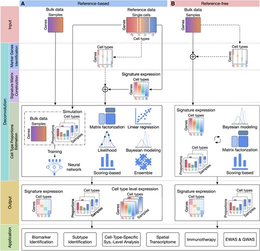
The high-level description of computational deconvolution methods and their applications. The two columns of the figure represent two major classes: (A) reference-based and (b) reference-free methods. The rows of the figure (separated by dashed lines) represent the input, the three steps of the deconvolution process, the output, and potential applications. The input of reference-based methods (A) includes bulk expression data and reference single-cell data, while reference-free methods (B) only require bulk data (top row). The deconvolution process starts by identifying the marker genes of the cell types (second row). After removing non-marker genes, deconvolution methods estimate the expression of each cell type and construct the signature matrix in which each column represents the expression of a cell type (third row). Finally, deconvolution methods infer the cell type proportions using various statistical and machine learning techniques (fourth row). The output of the deconvolution methods often includes both the signature matrix and the cell type proportion matrix in which each column represents the cell type proportions of a bulk sample (fifth row). The last row shows the potential applications of cellular deconvolution, including biomarker identification, cancer subtyping, cell-type-specific systems-level analysis, spatial transcriptome analysis, immunotherapy, and genetic and epigenetic association studies (GWAS and EWAS).
There are methods that do not require any additional input which we refer to as reference-free methods (right side of Figure 1). These include methods developed earlier, before actual single-cell data became available. Reference-free methods perform unsupervised learning of the bulk data to identify the marker genes and to infer both the cell-type signature matrix and cell type composition. Methods that only require the marker genes for the cell types are referred to as semi-reference-free methods. After computation, deconvolution methods often produce the following: (i) the cell type proportions, (ii) the signature matrix of the cell types and (iii) the expression of each sample in each cell type. We provide the technical details of individual methods in section Technical description of deconvolution methods.
Practical applications of cellular deconvolution
Biomarkers identification is an important application of cellular deconvolution (48). Many studies reported that important markers of cancer cells are highly correlated with immune cell compositions (49–51). These markers play important roles in regulating human immune response and could be potential targets for drug development. To identify new biomarkers, scientists usually look for the genes that have expression levels highly correlated with the CD8 T-cell tumor infiltration levels. One example is that MAGEA3 has been identified as a vaccine candidate for non-small cell lung carcinoma and melanoma (52). Cellular deconvolution analysis using TCGA data shows that MAGEA3 expression level is negatively correlated with CD8 T-cell infiltration level in non-small cell lung carcinoma while there is a positive correlation in melanoma (5). This is consistent with clinical trial results, in which MAGEA3 vaccine showed positive results in melanoma trials, and failed to improve progression-free survival of non-small cell lung carcinoma patients (52). Similarly, CTAG1B has been identified as a promising immuno-therapy candidate for melanoma because its expression is strongly correlated with CD8 T-cell infiltration (5). This approach also shows positive results for biomarkers identification in other diseases such as atherosclerosis (53), inflammatory bowel diseases (54), systemic lupus erythematosus (55), or discovery of damage-related or absorbed dose-dependent radiation research (56). In fact, cellular deconvolution can be applied to all existing bulk data independently of the disease to identify important biomarkers without the need of performing single-cell sequencing or other expensive experiments.
Cellular deconvolution can greatly impact the research field of cancer subtyping. It has been demonstrated that different subtypes of tumor samples showed distinct immune cell infiltrating patterns, where macrophages account for the largest proportion of immune cells in all five subtypes of breast cancer and bladder cancer samples (57). This is consistent with previous experimental studies that high infiltration of tumor-associated macrophages is a hallmark of inflammatory breast cancers (58). Cell type proportions in tumor samples can be of great assistance in identifying distinct cancer subtypes (59–61) that have different survival profiles (62,63). By identifying genes that are significantly correlated with changes in immune cell composition among cancer subtypes, pathway analysis can be used to identify the underlying mechanisms driving such heterogeneity. One can also deconvolve the bulk data expression profile into expression profiles for individual cell types. This deconvolution allows the investigation of the disease at cell type resolution using methods such as subtyping (64,65), regulatory network inference (66,67) or pathway analysis (68,69), which would enable the discovery of insights that could not be possible from bulk data.
Another application of cellular deconvolution is to improve the resolution of spatial transcriptome data, which has recently emerged as a bridge between molecular and histology data (70). Each spatial region or spot in spatial transcriptome data usually measures the average expression of multiple cells (71). The number of cells within each spot can range from 30 in the popular Visium platform up to 200 for older spatial transcriptomics platforms (72). Using cellular deconvolution techniques, one can improve the resolution of spatial data by deconvolving each spatial region into smaller regions of cell types present in that area. This deconvolution is especially important for applications such as cell-to-cell/ligand–receptor interaction inference, in which the spatial distance among cells is taken into consideration by the method. The emergence of newer spatial technologies such as ComMX, Xenium and Merscope partially addresses these issues and may reduce the importance of deconvolution in these applications if they are widely adopted. Besides spatial transcriptome, cellular deconvolution can also be applied to other data types without abundant availability of single-cell resolution data such as ATAC-seq (73) or methylation (74).
Another potential application of cellular deconvolution is cancer immunotherapy. It has been shown that the composition of immune cells in the tumor microenvironment is a major contributor to the heterogeneity in cancer progression and treatment success (75). As immune cells infiltrate tumors to regulate their growth, their composition within the solid tumor is a strong predictor for a patient’s overall survival (3). It has been shown that the composition of immune cells in the tumor microenvironment is a major contributor to the heterogeneity in cancer progression and treatment success (75). As immune cells infiltrate tumors to regulate their growth, their composition within the solid tumor is a strong predictor for a patient’s overall survival (3). It has been demonstrated that a high level of macrophage infiltration is strongly associated with low survival of breast and bladder cancer patients (4,57,76). At the same time, higher levels of CD8 T-cell correlates with better survivals of melanoma and head and neck cancer patients (5). Histologists and clinicians currently rely on immunohistochemistry to detect the infiltrating lymphocytes and to determine the immune cell composition of cancer tissues. Immunohistochemistry techniques, however, rely on pre-selected markers, thus not ideal for detecting the fine-grained lymphocyte subsets. Single-cell profiling is becoming more affordable but it still presents a substantial cost (Supplementary Section S2). Flow sorting would be a much better approach that can be used to address this problem but it would also involve additional costs. Since tumor sequencing is done anyway for reasons related to treatment selection, deconvolution may be a suitable approach to determine the levels of infiltrating lymphocytes and to quantify the immune cell composition of cancer tissues. This allows for a comprehensive monitoring of tumor micro-environment, cancer progression, and response to cancer immunotherapy and treatments. In turn, this can lead to better strategies for cancer therapeutics and drug development.
Finally, cellular deconvolution can be applied to epigenome-wide and transcriptome-wide association studies (EWAS and TWAS). The estimated cell type proportion can be used as a fixed effect on EWAS and TWAS analysis (77). For example, to assess the relevance of the estimated cell type proportions in Alzheimer’s disease, Patrick et al. (78) included the estimated proportions as confounding factors to neuropathology-related genes, namely amyloid beta and tau proteins. The result shows a substantial reduction in the number of genes associated with amyloid beta, suggesting that the genes found without adjusting for cellular heterogeneity are likely to be false positives since their variance can be significantly explained away by variability in cell type proportions. These genes may be exclusively expressed in neurons and therefore have lower expression levels in Alzheimer’s patients due to compositional changes of cell types during neurodegeneration. Such genes are not actionable targets for the treatment of Alzheimer’s since they are not causally involved in the biological mechanism underlying Alzheimer’s disease, but are only brought up by the confounding effects of cell types.
Current strategies for method validation
Figure 2 shows the high-level description of strategies that have been used to assess the performance of deconvolution methods. Overall, assessment approaches can be classified into five main categories:
simulating bulk data from scRNA-Seq data
using data from a mixture of cell lines
analyzing datasets that include both RNA-Seq and scRNA-Seq data
using datasets that have both bulk transcriptome data and flow cytometry counter data, and
performing enrichment analysis using clinical variables.
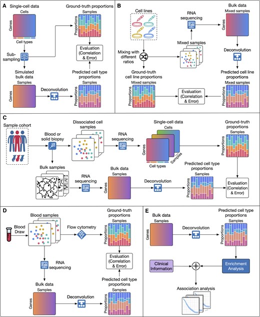
Common evaluation strategies used by current deconvolution methods. Overall, assessment approaches can be classified into five main categories: (A) simulating bulk data from scRNA-Seq data, (B) using data from a mixture of cell lines, (C) analyzing datasets that include both RNA-Seq and scRNA-Seq data, (D) using datasets that have both bulk transcriptome data and flow cytometry counter data and (E) performing enrichment analysis using clinical variables. For the first four scenarios, the ground truth proportions of the cell types are known and thus can be used to directly assess the accuracy of deconvolution methods. In the fifth scenario, deconvolution methods are indirectly assessed using expert knowledge and/or enrichment analysis.
For the first four approaches, the ground truth proportions of the cell types are known and thus can be used to directly assess the accuracy of deconvolution methods. The fifth approach relies on domain experts to interpret the deconvolution results to indirectly assess the performance of deconvolution methods. We also provide the available data for each validation approach in Supplementary Table S1.
The first approach simulates bulk data from purified samples or single-cell data. For each simulated bulk dataset and sample, the cell type composition is known and thus can be used a posteriori to evaluate the performance of deconvolution methods (74,79–93). To quantify the accuracy of a method, this approach compares the cell type proportions estimated for each bulk sample against the ground truth using either Pearson correlation, absolute error, or both. The performance of each deconvolution method is measured by the average correlation (the higher the better) and/or average mean absolute error (the lower the better) across all simulated bulk samples. Although this approach has the ability to simulate a large number of samples, it may not reflect real-world scenarios. In addition, simulation is subjected to bias because simulated data is generated based on some assumptions which are usually identical with the assumptions made in designing the approach. Presumably, any algorithm would be the best, when applied to data that was simulated based on the same set of assumptions.
The second approach uses datasets that have both the expression profiles of pure cell lines and the in vitro mixture of these cell lines (84,88,91,94–97). To generate this type of data, biologists culture the pure cell lines independently and then mix the cell lines with pre-defined ratios to generate bulk samples. Then, they generate the gene expression profiles of both bulk samples and the pure cell lines. In this evaluation approach, the reference-based methods use the gene expression profiles of pure cell lines to construct the signature matrix and then estimate the cell type proportions in the bulk samples. The accuracy of these methods is evaluated by comparing the estimated proportions against the pre-defined ratios. This approach is more realistic than using simulation but the disadvantage of this approach is the low throughput of the mixture generation step. Datasets generated in vitro usually have a low number of samples and cell types, which often leads to overfitting.
The third approach uses datasets that have both bulk RNA-Seq and scRNA-Seq data generated from the same tissue samples (81,84,98,99). The single-cell data are often used for two purposes. First, the cell type proportions calculated from single-cell data can be treated as ground truth to assess the accuracy of deconvolution methods. Second, a subset of single-cell data can be used to construct the signature matrix for reference-based methods. Although the matched RNA-Seq and scRNA-Seq could theoretically provide a reasonable scenario to evaluate the performance of the deconvolution methods, the availability of such data is limited. In addition, because the same single-cell data are used as ground truth and as the input of reference-based methods, this approach can potentially lead to data leakage and overfitting. Furthermore, there are limitations with this approach due to biases in the single-cell data since some cell types are inherently more sensitive to dissociation than others.
The fourth approach uses datasets that have both bulk data and flow cytometry (57,81,83,95,100–106). Flow cytometry data measures the counts of each cell type in the bulk samples and thus can provide an approximation of true cell type composition in the bulk samples. Cell type proportions calculated from the flow cytometry can be used as ground truth to assess the accuracy of deconvolution methods. In this approach, the reference-based methods usually need to construct the signature matrix using another dataset if the pure cell type samples are not available. The disadvantage of this approach is that the cytometry data is generally available only for blood samples. Using this validation approach alone could introduce bias to the deconvolution methods, where they often overfit to blood data and thus might provide inaccurate results for samples coming from other tissues.
The last approach is used when the bulk data does not have matched single-cell or flow cytometry data. In those cases, other information such as clinical variables, survival information, and treatment/disease status can be used to indirectly assess the performance of the deconvolution methods (57,86,96,100,106–109). This can be done by associating the estimated cell type proportions with important clinical variables and/or reported discoveries from the literature. As such, one can use the inferred cell type proportions to determine the subtype of patients and then validate that the discovered subtypes have significantly different survival profiles. Another indirect validation approach is to confirm previously reported results, such as the association of treatments’ efficacy with known shifts in tissue composition. For example, the group treated with an immunotherapy agent should have an elevation in immune cell proportions (89,110), or type 2 diabetes patients are expected to show a decrease in the proportion of beta cells (79,111). Due to its complexity, this approach is often considered as the last resort to be used only when there is no available data for a direct quantitative assessment.
Technical description of deconvolution methods
Figure 3A shows the key characteristics of the 53 deconvolution methods including method category, implementation platform, required input, output, and underlying inference algorithm. We provide a description of individual methods, including their input, output, and data transformations and pre-processing steps in the Supplementary Note and Supplementary Table S6. Most of the reviewed methods (41 out of 53) require users to provide raw read counts (discrete integers). One method (quanTIseq) asks users to provide the sequencing file (.fastq) while the remaining methods allow users to provide normalized data (TPM-normalized or microarray).

Key characteristics and technical evaluation of cellular deconvolution methods. (A) Method characterization according to implementation, input, output, embedded reference and the underlying algorithm. (B) Performance assessment based on five criteria: the accuracy of the predicted cell type proportions, the scalability in analyzing large input sizes, the stability (opposite of crash rate and other errors), the consistency of the predicted cell type proportions using different initializations, and the usability as code quality and ease of use. *Abbreviations: S: signature matrix; F: full cell-type expression matrix; PCA: principal component analysis; NMF: non-negative matrix factorization; CLS: constrained least squares; SVR: support vector regression; MLE: maximum likelihood estimation; DNN: deep neural network; ensemble: combination of multiple methods; scoring: enrichment using marker sets. W prefix: weighted. R prefix: regularized. ***BisqueRef requires scRNA data of at least two subjects as input. TICPE requires cancer cell expression, normal cell expression, immune cell expression and marker gene sets as input.
In total, we review 39 reference-based methods (MuSiC (79), DWLS (80), AdRoit (112), spatialDWLS (113), Scaden (81), LinDeconSeq (109), DigitalDLSorter (82), AutoGeneS (114), RNA-Sieve (83), DecOT (111), BayICE (94), DeconPeaker (73), SCDC (84), DAISM-DNN (115), CPM (85), MOMF (86), BisqueRef (116), deconvSeq (101), DeCompress (87), DeMixT (117), CIBERSORT (107,108), MethylResolver (104), MIXTURE (105), FARDEEP (118), NITUMID (110), MySort (119), PREDE (57), quanTIseq (106), DeconRNASeq (120), DCQ (88), dtangle (102), DESeq2’s unmix (121), ARIC (100), EMeth (122), ImmuCellAI (89), EPIC (103), TICPE (90), BayesPrism (98), Bseq-SC (99)), 10 reference-free approaches (Linseed (123), TOAST (91,92), debCAM (124), CellDistinguisher (125), deconf (126), BayCount (127), BayesCCE (74), ReFACTor (93), DeconICA (128), SMC (97)) and 4 semi-reference-free techniques (Deblender (95), MCP-counter (129), BisqueMarker (116), DSA (96)).
Three main steps of cellular deconvolution
The workflow of a deconvolution method usually consists of three main steps: (i) cell-type markers identification, (ii) signature matrix construction and (iii) cellular deconvolution. The input of deconvolution methods includes the bulk expression data to be deconvolved, reference single-cell data and marker genes of each cell type.
In the first step, deconvolution methods aim at determining the marker genes for the available cell types of the tissue. If a reference single-cell dataset is available, the marker genes can be determined by performing a comparative analysis among cell types. The marker genes can also be derived from the literature and/or from single-cell databases. If neither reference data nor prior knowledge are available, deconvolution methods can use unsupervised learning and pattern recognition to determine both cell types and marker genes from the bulk data.
The second step focuses on computing the expression of each cell type. The expression of the cell types is often represented by a signature matrix S in which columns represent cell types and rows represent marker genes. When the reference single-cell data and the cell type label are available, the expression of each cell type (each column of S) is typically computed by averaging the expression values of all cells belonging to the underlying cell type. When the reference data is available without cell type label, unsupervised clustering can be performed to determine the cell groups. When the reference single-cell data is not available, reference-free and semi-reference-free methods estimate the signature matrix directly from the bulk data using unsupervised learning.
In the third step, the expression of each bulk sample is decomposed into a linear combination of the expression of all cell types in the tissue, in which the coefficients are considered cell type proportions. Specifically, b = S × p, as described by Equation (1). When users input a bulk dataset that has m samples, the formula becomes as follows:
or B = S × P in which B is a matrix of n genes by m bulk samples that represents the input bulk dataset and P is a matrix of k cell types by m samples that represents the cell type proportions of the samples. For reference-free methods, where the signature matrix S is pre-computed from reference single-cell data, P can be estimated by minimizing the difference between B and S × P. For reference-free techniques, where the reference single-cell data is not available, both S and P are iteratively and simultaneously estimated from the bulk data. The output of the deconvolution methods often includes both the signature matrix S and the cell type proportion matrix P.
Identification of cell type markers
Among the reference-based methods listed in Figure 3, 10 methods, MuSiC, Scaden, DigitalDLSorter, RNA-Sieve, BayesPrism, DecOT, DAISM-DNN, MOMF, DESeq2’s unmix and EMeth, use all genes for their deconvolution process and thus omit the step of marker identification. The other 16 methods, spatialDWLS, CIBERSORT, CIBERSORTx, MethylResolver, MIXTURE, FARDEEP, NITUMID, MySort, quanTIseq, DeconRNASeq, DCQ, dtangle, PREDE, ImmuCellAI, EPIC and TICPE, require users to provide the marker genes. The remaining reference-based methods identify the marker genes by comparing cells of the underlying cell type against all remaining cells using common comparative analysis: t-test, likelihood-ratio, Wilcoxon Rank Sum, ANOVA, fold change, signal-to-noise ratio, co-linearity score, multi-objective genetic algorithm and Wald test.
Reference-free methods perform unsupervised learning on the bulk data to identify the cell types and their markers. Linseed and debCAM project the gene data onto a low-dimensional space and then identify the genes close to the corner of the smallest simplex as marker genes. CellDistinguisher computes the gene-gene conditional expression matrix from the bulk data input and identifies the marker genes as ones that correspond to the most extreme vectors in this matrix. BayesCCE and ReFACTor perform gene filtering to remove irrelevant genes. The remaining reference-free methods, TOAST, deconf, BayCount, DeconICA and SMC, use all genes provided in the bulk data for their deconvolution.
Semi-reference-free methods (Deblender, MCP-counter, BisqueMarker and DSA) allow users to provide the marker genes for the cell types. If users do not provide the markers, then MCP-counter will use the embedded markers for 10 stromal cell types whereas Deblender performs unsupervised clustering to partition the genes into different groups that represent different cell types. Genes that are closest to each cluster center are considered marker genes.
Signature matrix construction
Methods that include a signature matrix in the deconvolution process either compute and fix the signature matrix prior to calculating the cell type proportions, or simultaneously estimate both the signature matrix and cell type proportions. There are a few exceptions in which deconvolution methods do not use the signature matrix for the process of estimating the proportions. These include Scaden, DigitalDLSorter, DAISM-DNN, TICPE, Linseed, ReFACTor, BisqueMarker and DSA.
As we mentioned above, the deconvolution is formulated as B = S × P where B is the bulk data, S is the signature matrix, and P is the proportion matrix. Many reference-based methods construct the signature matrix from the reference single-cell data (those with checkmark symbol in the scRNA-Seq column in Figure 3). They calculate the signature matrix by averaging the expression of cells belonging to the same cell types. The rest of the reference-based methods require users to provide the signature matrix (those without the checkmark symbol in the scRNA-Seq but with F and S in the CT Expr). F and S matrices are both cell type expression matrices but F matrix includes the expression of all genes whereas S matrix only contains marker genes. The marker genes in the S matrix are expected to be mutually exclusive, i.e., these marker genes are expressed in one cell type but not in others. Although F and S matrices are conceptually interchangeable, providing a type of input different from what is specified in the software manual can have unexpected effects on the software. For example, some F methods (DESeq2, dtangle, PREDE, EMeth) crash when we provide the S matrix. In contrast S methods can take substantially longer time to run when we provided them with F matrix. Therefore, we suggest users to provide the input as specified in the manual of each software.
As we mentioned above, the deconvolution is formulated as B = S × P where B is the bulk data, S is the signature matrix, and P is the proportion matrix. Among the reference-based methods, many require users to provide the signature matrix (those with F and S in the CT Expr in Figure 3). Some of them, including CIBERSORT, CIBERSORTx, MethlyResolver, NITUMID, MySort, quanTIseq, Bseq-SC, DCQ and ImmuCellAI, also have the signature matrix of certain cell types embedded in their software. Otherwise, reference-based methods construct the signature matrix from the reference single-cell data. Most of them calculate the signature matrix by averaging the expression of cells belonging to the same cell types. The rows in this matrix can be all genes or just the biomarkers as described in the previous section. When only the biomarkers are used in the signature matrix, it is expected that they are mutually exclusive.
Without the reference single-cell data, reference-free and semi-reference-free methods aim at simultaneously estimating both the signature matrix and cell type proportions from the bulk data without using any external information. debCAM uses the marker genes to construct a simplex, and then projects the marker genes onto the axes and averages the projected values to create the expression of the cell type. Deblender simply averages the expression of the marker genes in the bulk data to estimate the expression of each cell type. CellDistinguisher, after identifying marker genes, projects the input matrix onto the space spanned by its row vectors corresponding to cell type-specific markers, resulting in the cell type signature matrix. TOAST and deconf use non-negative matrix factorization to iteratively optimize S and P until the absolute errors or square errors reach a certain threshold. The three Bayesian methods, BayCount, BayesCCE and SMC, model the bulk data to follow a probabilistic distribution whose parameters and then iteratively update both the signature and proportion matrices to maximize the likelihood functions.
Estimating cell type proportions
Given the mathematical definition of the deconvolution, B = S × P, many methods aim at minimizing the squared errors. There are 16 deconvolution methods that are based on constrained least squares (CLS in Figure 3) with the constraints that the values of cell type proportions are non-negative and sum up to one. To obtain the cell type proportions, these methods apply classical quadratic programming algorithms. One drawback of the CLS model is that it can be influenced by outliers or genes with abnormally high expression. To address this, five methods, MuSiC, DWLS, spatialDWLS, LinDeconSeq and EPIC, use the weighted constrained least squares (W-CLS) model to put less weight on genes with high variance. AdRoit and DCQ also apply the regularized constrained least squares (R-CLS) model that automatically shrinks irrelevant cell types using Ridge regression and elastic net, respectively.
CLS, W-CLS and R-CLS models display a good performance generally when S is well conditioned, i.e. its constituent cell types are highly distinctive with mutually exclusive markers. To avoid relying on such assumptions, many methods have introduced more sophisticated techniques to estimate cell type proportions, including support vector regression (SVR), deep neural networks (DNN), maximum likelihood estimation (MLE), Bayesian modeling, ensemble, scoring and matrix decomposition.
Eight SVR methods include AutoGeneS, CPM, CIBERSORT, CIBERSORTx, MIXTURE, MySort, Bseq-SC, and ARIC. In comparison to the CLS models, the objective function of SVR aims to minimize the coefficients (cell type proportions) instead of the squared errors. The SVR model regularizes the coefficients using Ridge regression (L2–norm), while the error term is handled by an extra constraint such that the error must lie within a specified margin. Compared to CLS, the SVR model has the following advantages: (i) is robust against noise, (ii) can automatically select important genes from the signature matrix and (iii) can account for multicollinearity between cell types.
The three DNN methods, Scaden, DigitalDLSorter and DAISM-DNN, require users to provide the reference single-cell data with known cell type labels. From the single-cell data, these methods randomly select a subset of the single cells to generate both the bulk expression and the cell type proportions. The process is repeated millions of times to generate sufficient training data for the model. These approaches do not require a well-conditioned signature matrix to estimate cell type proportions, but they do need a sufficiently large single-cell dataset to simulate millions of bulk samples for the neural network. Such requirement is specified in Scaden method’s manuscript (81) and we also observe similar data generation strategy in the source code of DigitalDLSorter (82) and DAISM-DNN (115).
The four MLE methods, RNA-Sieve, deconvSeq, DeMixT and EMeth, model the expression data using probabilistic distributions and then compute cell type proportions by maximizing the likelihood function. The estimation can be done by solving a system of gradient equations or using the classical Expectation Maximization (EM) algorithm. The performance of these MLE-based methods depends on the correctness of the underlying assumptions of the data (130). In addition, the likelihood function with a large number of parameters may be hard to optimize, making MLE methods slow and computationally expensive (131).
The five Bayesian methods, BayesPrism, BayICE, BayCount, BayesCCE and SMC, combine the probabilistic models with prior knowledge of cell type proportions. In addition to modeling the observed expression data, the five Bayesian approaches also model the cell type proportions to follow a prior distribution in each tissue. These approaches use sampling techniques, such as Gibbs or Markov chain Monte Carlo, to sample the cell type proportions from the prior distribution and then calculate the likelihood of the observed expression data. In the end, these approaches calculate the cell type proportions that maximize the likelihood of the observed expression data. Bayesian approaches are not applicable to tissues in which the distribution of cell type proportions (prior knowledge) is not known.
The three methods, SCDC, DecOT and Decompress, use the ensemble strategy to estimate the cell type proportions. SCDC and DecOT create multiple signature matrices from different single-cell datasets and then use each signature matrix to deconvolve the bulk data. These approaches then combine all estimated cell type proportions using a W-CLS model to determine the final proportions. Decompress uses six different methods, deconf, CellDistinguisher, TOAST, Linseed, DeconICA, and DESeq2’s unmix, to estimate the cell type proportions and then choose the estimation that has the smallest squared error. Choosing an appropriate ensemble technique remains a challenge and it does not guarantee to provide better results than those obtained from a single analysis. For example, SCDC uses MuSiC as part of their ensemble strategy to estimate the cell type proportions, but SCDC does not perform as well as MuSiC in our experiments (Supplementary Figures S2–S11).
The five methods, dtangle, TICPE, Linseed, MCP-Counter and DSA, introduce a new strategy named scoring to estimate the cell type proportions. Given the markers, Linseed, MCP-Counter and DSA calculate the score for each cell type by taking the mean expression of its markers in the bulk sample. Linseed and DSA normalize these scores to represent the cell type proportions. In contrast, dtangle and TICPE compute a relative abundance ratio for each pair of cell types and then estimate the cell type proportions using multivariate logistic and Gauss-Newton method. Scoring-based methods might perform well on tissues with few cell types but are not ideal in deconvolving tissues with a more complex mixture of many cell types, especially when the cell types have overlapping markers. As shown in Supplementary Figures S5-S10, scoring-based methods have relatively lower accuracy in CELLxGENE tissues where the data have more cell types compared to Tabula Sapiens tissues.
The remaining eleven methods use matrix decomposition to simultaneously estimate both the cell type proportions and the signature matrix. Among these, there are nine NMF and two PCA methods. The NMF methods typically initialize the matrices S and P and then iteratively update them by minimizing the discrepancy between B and S × P in Equation (2). The two PCA techniques, BisqueMarker and ReFACTor, decompose the bulk data to obtain a k-rank approximation in which k represents the number of cell types. The values of the first k PCs represent the cell type proportions of all samples. These matrix decomposition-based methods may fail to provide a unique optimal solution because the N-dimensional polygon—as defined by the various constraints and objectives—is not convex. Six methods, debCAM, CellDistinguisher, deconf, ReFACTor, DeconICA and Deblender, return cell type proportions without cell type labels. In these cases, users need to perform additional steps to match the proportions with actual cell types in the bulk samples.
Performance assessment and analysis results
Benchmarking workflow and implementation
While researchers mainly seek to use the most accurate method, scalability, reproducibility (consistency), installation issues, crashes, poor documentation and fine-tuning many parameters might prevent users from trying or effectively deploying a given method. In order to capture all the aspects mentioned above when comparing various methods, we define five different metrics that quantitatively evaluate each method: (i) accuracy—how well the method can correctly estimate the cell type proportions, (ii) scalability—how well the method can scale to an increasing number of bulk samples, (iii) consistency—how robust the method is against noise and random factors, (iv) stability—how often the method crashes or returns errors and (v) usability—how easy it is to install the software and to analyze the data. These metrics aim to capture the usefulness of the methods from the perspectives of both computational scientists and medical practitioners/life researchers.
Figure 4 shows the workflow of the evaluation procedure. To perform a comprehensive assessment, we evaluate the methods using a total of 30 tissues from two data sources: Tabula Sapiens (132) and CELLxGENE (133). Table 1 shows the details of the data used in our analysis. For Tabula Sapiens data, we choose tissues that have at least two donors, resulting in a total of 20 tissues, 15 donors and 135 cell types. For the CELLxGENE data, we choose tissues that have at least five donors and ten cell types. This results in 10 tissues, 48 human donors and 148 cell types. For each tissue, we use the data from one donor to generate reference single-cell expression, and the data from the remaining donors to generate bulk samples. To generate a bulk data sample, we first generate cell type proportions and then select cells from the single-cell data of the first donor to match the pre-defined proportions. We then use the deconvolution methods to estimate the cell type proportions of the generated bulk samples. We also provide additional information for methods that require extra input, including the number of cell types, single-cell data, signature matrix, or cell-type-specific markers. After the deconvolution methods finish their analyses, we use the true cell type proportions to quantitatively assess the performance of the deconvolution methods.
Description of the 30 tissues from Tabula Sapiens and CELLxGENE included in the evaluation
| Tissue | #Donors | #UMIs | #Genes | #Types | Description | |
|---|---|---|---|---|---|---|
| Tabula Sapiens | ||||||
| 1. | Bladder | 3 | 13219 | 2739 | 9 | T cell, macrophage, myofibroblast cell, bladder urothelial cell, smooth muscle cell, fibroblast, pericyte cell, mast cell, mature NK T cell |
| 2. | Blood | 6 | 9100 | 1866 | 6 | erythrocyte, classical monocyte, neutrophil, memory B cell, plasma cell, platelet |
| 3. | Bone Marrow | 3 | 11848 | 2600 | 8 | plasma cell, hematopoietic stem cell, erythroid progenitor cell, mature NK T cell, granulocyte, naive B cell, CD8 positive alpha beta T cell, CD4 positive alpha beta T cell |
| 4. | Eye | 3 | 17357 | 3286 | 7 | conjunctival epithelial cell, eye photoreceptor cell, Muller cell, retinal blood vessel endothelial cell, keratocyte, corneal epithelial cell, melanocyte |
| 5. | Fat | 2 | 13353 | 3247 | 4 | fibroblast, endothelial cell, macrophage, myofibroblast cell |
| 6. | Large Intestine | 2 | 16385 | 3764 | 5 | CD8 positive alpha beta T cell, fibroblast, paneth cell of colon, B cell, gut endothelial cell |
| 7. | Liver | 2 | 10123 | 2729 | 2 | endothelial cell of hepatic sinusoid, hepatocyte |
| 8. | Lung | 3 | 9102 | 1849 | 3 | type II pneumocyte, mature NK T cell, adventitial cell |
| 9. | Lymph Node | 3 | 8458 | 2302 | 9 | B cell, effector CD4 positive alpha beta T cell, regulatory T cell, plasma cell, neutrophil, macrophage, CD1c positive myeloid dendritic cell, intermediate monocyte, mast cell |
| 10. | Muscle | 3 | 15256 | 3282 | 11 | mesenchymal stem cell, skeletal muscle satellite stem cell, capillary endothelial cell, pericyte cell, fast muscle cell, macrophage, endothelial cell of vascular tree, slow muscle cell, endothelial cell of artery, tendon cell, endothelial cell of lymphatic vessel |
| 11. | Pancreas | 2 | 7477 | 2024 | 7 | pancreatic acinar cell, T cell, endothelial cell, myeloid cell, pancreatic stellate cell, B cell, pancreatic ductal cell |
| 12. | Prostate | 2 | 10319 | 2532 | 6 | basal cell of prostate epithelium, epithelial cell, club cell, erythroid progenitor cell, luminal cell of prostate epithelium, endothelial cell |
| 13. | Salivary Gland | 2 | 9155 | 2564 | 10 | acinar cell of salivary gland, pericyte cell, mature NK T cell, fibroblast, endothelial cell of lymphatic vessel, adventitial cell, endothelial cell, monocyte, duct epithelial cell, basal cell |
| 14. | Skin | 2 | 19725 | 3031 | 8 | macrophage, stromal cell, mast cell, muscle cell, CD1c positive myeloid dendritic cell, endothelial cell, naive thymus derived CD8 positive alpha beta T cell, regulatory T cell |
| 15. | Small Intestine | 2 | 10034 | 2480 | 4 | CD8 positive alpha beta T cell, B cell, paneth cell of epithelium of small intestine, fibroblast |
| 16. | Spleen | 3 | 13680 | 2475 | 13 | macrophage, intermediate monocyte, endothelial cell, memory B cell, classical monocyte, neutrophil, naive B cell, plasma cell, type I NK T cell, mature NK T cell, innate lymphoid cell, regulatory T cell, hematopoietic stem cell |
| 17. | Thymus | 2 | 8746 | 2160 | 9 | medullary thymic epithelial cell, fibroblast, macrophage, vascular associated smooth muscle cell, plasma cell, vein endothelial cell, capillary endothelial cell, endothelial cell of artery, monocyte |
| 18. | Tongue | 2 | 8706 | 1971 | 5 | leukocyte, fibroblast, vein endothelial cell, pericyte cell, capillary endothelial cell |
| 19. | Trachea | 2 | 9850 | 2395 | 3 | endothelial cell, ciliated cell, basal cell |
| 20. | Vasculature | 2 | 8794 | 2414 | 6 | fibroblast, smooth muscle cell, macrophage, pericyte cell, mast cell, mature NK T cell |
| CELLxGENE | ||||||
| 21. | Anterior Cingulate Cortex | 5 | 15350 | 3360 | 18 | lamp5 GABAergic cortical interneuron, sncg GABAergic cortical interneuron, caudal ganglionic eminence derived GABAergic cortical interneuron, vip GABAergic cortical interneuron, L5 extratelencephalic projecting glutamatergic cortical neuron, near projecting glutamatergic cortical neuron, corticothalamic projecting glutamatergic cortical neuron, L6b glutamatergic cortical neuron, astrocyte of the cerebral cortex, cerebral cortex endothelial cell, vascular leptomeningeal cell, microglial cell, oligodendrocyte, oligodendrocyte precursor cell, L2/3-6 intratelencephalic projecting glutamatergic cortical neuron, chandelier pvalb GABAergic cortical interneuron, pvalb GABAergic cortical interneuron, sst GABAergic cortical interneuron |
| 22. | Basal Zone of Heart | 6 | 5867 | 2028 | 16 | native cell, fibroblast, smooth muscle cell, pericyte, myeloid cell, endocardial cell, endothelial cell of artery, vein endothelial cell, endothelial cell, fetal cardiomyocyte, cardiac muscle cell, neuron, cardiac mesenchymal cell, innate lymphoid cell, capillary endothelial cell, mesothelial cell of epicardium |
| 23. | Fimbria of Uterine Tube | 5 | 5400 | 1739 | 11 | natural killer cell, endothelial cell, stromal cell, smooth muscle cell, pericyte, secretory cell, endothelial cell of lymphatic vessel, macrophage, B cell, mast cell, ciliated epithelial cell |
| 24. | Heart Left Ventricle | 12 | 3801 | 1624 | 10 | native cell, cardiac muscle cell, mural cell, mast cell, cardiac neuron, endothelial cell, fibroblast of cardiac tissue, myeloid cell, lymphocyte, fat cell |
| 25. | Liver | 14 | 2101 | 1063 | 11 | naive thymus derived CD4 positive alpha beta T cell, natural killer cell, CD8 positive alpha beta cytotoxic T cell, CD8 positive alpha beta memory T cell, B cell, gamma delta T cell, T cell, memory T cell, plasma cell, plasmacytoid dendritic cell, regulatory T cell |
| 26. | Middle Temporal Gyrus | 5 | 21303 | 5745 | 18 | astrocyte of the cerebral cortex, oligodendrocyte, vascular leptomeningeal cell, microglial cell, oligodendrocyte precursor cell, cerebral cortex endothelial cell, near projecting glutamatergic cortical neuron, corticothalamic projecting glutamatergic cortical neuron, L6b glutamatergic cortical neuron, L5 extratelencephalic projecting glutamatergic cortical neuron, caudal ganglionic eminence derived gabaergic cortical interneuron, vip GABAergic cortical interneuron, sncg GABAergic cortical interneuron, lamp5 GABAergic cortical interneuron, sst GABAergic cortical interneuron, pvalb GABAergic cortical interneuron, chandelier pvalb GABAergic cortical interneuron, L2/3-6 intratelencephalic projecting glutamatergic cortical neuron |
| 27. | Primary Auditory Cortex | 5 | 12219 | 2768 | 18 | lamp5 GABAergic cortical interneuron, caudal ganglionic eminence derived GABAergic cortical interneuron, vip GABAergic cortical interneuron, sncg GABAergic cortical interneuron, L5 extratelencephalic projecting glutamatergic cortical neuron, near-projecting glutamatergic cortical neuron, corticothalamic-projecting glutamatergic cortical neuron, L6b glutamatergic cortical neuron, astrocyte of the cerebral cortex, vascular leptomeningeal cell, cerebral cortex endothelial cell, microglial cell, oligodendrocyte, oligodendrocyte precursor cell, L2/3-6 intratelencephalic projecting glutamatergic cortical neuron, chandelier pvalb GABAergic cortical interneuron, pvalb GABAergic cortical interneuron, sst GABAergic cortical interneuron |
| 28. | Primary Somatosensory Cortex | 5 | 13427 | 2903 | 18 | lamp5 GABAergic cortical interneuron, sncg GABAergic cortical interneuron, caudal ganglionic eminence derived gabaergic cortical interneuron, vip GABAergic cortical interneuron, L5 extratelencephalic projecting glutamatergic cortical neuron, near projecting glutamatergic cortical neuron, corticothalamic projecting glutamatergic cortical neuron, L6b glutamatergic cortical neuron, astrocyte of the cerebral cortex, vascular leptomeningeal cell, cerebral cortex endothelial cell, microglial cell, oligodendrocyte precursor cell, oligodendrocyte, L2/3-6 intratelencephalic projecting glutamatergic cortical neuron, chandelier pvalb GABAergic cortical interneuron, pvalb GABAergic cortical interneuron, sst GABAergic cortical interneuron |
| 29. | Primary Visual Cortex | 5 | 9811 | 2164 | 18 | lamp5 GABAergic cortical interneuron, sncg GABAergic cortical interneuron, caudal ganglionic eminence derived GABAergic cortical interneuron, vip GABAergic cortical interneuron, L5 extratelencephalic projecting glutamatergic cortical neuron, near-projecting glutamatergic cortical neuron, corticothalamic-projecting glutamatergic cortical neuron, L6b glutamatergic cortical neuron, astrocyte of the cerebral cortex, cerebral cortex endothelial cell, oligodendrocyte precursor cell, vascular leptomeningeal cell, microglial cell, oligodendrocyte, L2/3-6 intratelencephalic projecting glutamatergic cortical neuron, chandelier pvalb GABAergic cortical interneuron, pvalb GABAergic cortical interneuron, sst GABAergic cortical interneuron |
| 30. | Small Intestine | 6 | 9953 | 2215 | 10 | T cell, B cell, enterocyte, macrophage, dendritic cell, endothelial cell of lymphatic vessel, neuron, fibroblast, blood vessel endothelial cell, enteroendocrine cell |
The first column shows the data source while the first column the name of the tissue. The third column shows the number of donors from which a tissue was collected from. The remaining columns show the average number of unique molecular identifiers (UMIs) detected per cell, average number of genes detected per cell, number of cell types, and cell type description.
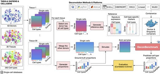
The evaluation procedure of cellular deconvolution methods using data from the Tabula Sapiens and CELLxGENE. The data has the single-cell expression data of 283 cell types from 30 tissues and 63 donors. For each tissue, we use the expression data of the donor that has all cell types to generate the single-cell data, and use the expression data of the remaining donors to generate bulk data. For each of the generated datasets, we have both reference single-cell data and bulk samples in which cell type proportions are known and thus can be used a posteriori to quantitatively evaluate the deconvolution methods. We also implement an R package, named DeconBenchmark (red box to the right of the figure), in which the implementation and dependencies of all methods are pre-installed and containerized using Docker and Singularity.
We also provide an R package, named DeconBenchmark, that includes the complete implementation of 50 deconvolution methods. We exclude three methods, DCQ, TICPE and SMC, from the package because they either are not available, or the code does not execute. The package gives readers instant access to all cellular deconvolution methods in a convenient and readily available manner. The package can be easily expanded to include new methods in the future if users wish to do so. The package is designed to allow researchers to: (i) test and evaluate cellular deconvolution methods without any installation steps regardless of their dependencies and platform, (ii) use the same standardized input and output formats for all methods, (iii) generate results from multiple methods and (iv) containerize and benchmark a new deconvolution method against all available methods. To standardize the input and output of the deconvolution methods, we provide a wrapper for each method in a containerized environment. This also allows users to avoid conflicts among the methods’ environment and dependencies. More details about the package can be found on the package’s GitHub page (https://github.com/tinnlab/DeconBenchmark).
Result summary
Figure 3 shows the key characteristics of the 53 deconvolution methods. Figure 3A shows the method category, implementation platform, required input, output, and underlying inference algorithm. Figure 3B shows a technical evaluation of deconvolution methods. Figure 3B shows the assessment results using the five metrics: (i) accuracy, (ii) scalability, (iii) consistency, (iv) stability and (v) usability. We assess the accuracy of the methods using a total of 30 datasets of the 30 different tissues (Table 1)—one per tissue. We also generate 20 more datasets from CELLxGENE tissues to investigate the impact of incomplete reference data. To measure the scalability of the methods, we generate 80 more datasets with different numbers of bulk samples (100, 250, 500 and 1000 samples).
The overall score is the weighted average of the five metrics: |$Overall=\frac{1}{6}(3 \times Accuracy + Scalability + Consistency + \frac{Stability + Usability}{2})$|. The Accuracy metric measures how accurate the method is while the remaining four metrics measure its reliability. Among the remaining four metrics, Scalability measures whether the method can analyze large datasets while Consistency measures its robustness against noise. Stability and Usability both measure the reliability of the software (crash and documentation, respectively). In principle, a researcher who generally analyzes smaller datasets would not care about scalability. Similarly, a computer scientist who is used to debugging and working with command line software would perhaps tolerate a lower usability than a life scientist. However, all users would care about accuracy. For this reason, we tuned the weights so that Accuracy accounts for 50% of the Overall score and the other four metrics account for the remaining 50%. Scalability, Consistency and the sum (Stability + Usability) are weighted equally in our formula.
For methods that require the same type of input, we sort them in descending order of the overall score. DWLS and MuSiC have the highest overall scores among methods that require single-cell data as reference. MuSiC and DWLS are also reported as the top performers in a benchmarking study for tumor microenvironment deconvolution (37). For methods that require the signature matrix (marked as S in CT expr* column), CIBERSORT has the highest score. For methods that require the full cell-type expression matrix (marked as F in CT expr* column), DESeq2’s unmix has the highest score. According to our results, Linseed and MCP-counter have the highest overall scores among reference-free and semi-reference-free methods, respectively.
In general, reference-based methods outperform reference-free, and semi-reference-free methods. This is because reference-based methods can leverage the additional information from high-quality single-cell data to refine their inference. Interestingly, among the reference-based methods, the best methods are based on linear regression models. As shown in Figure 3, linear models dominate the list of top methods that have the best scores. The most important factor affecting method performance is how each method handles noise and avoids overfitting. The top two methods, MuSiC and DWLS, both use the Weighted Constrained Least Squares (W-CLS) model for a gene weighting scheme to minimize the impact of outliers. Data processing and hyperparameters also play significant roles. For example, CPM and CIBERSORT both use Support Vector Regression (SVR) but they differ in two aspects that lead to differences in performance. CIBERSORT uses ν-SVR (a variation of SVR), in which the added parameter ν to control the number of support vectors for optimizing the loss function. Another difference is that CIBERSORT pre-processes the reference data to keep only marker genes of the cell types in the signature matrix. Finally, implementation also matters. Even when using the same machine learning technique, a better implementation can significantly influence the scalability, stability, and many other metrics of the software.
In the following sections, we provide the details of all metrics and discuss the technical evaluation of the methods.
Accuracy
We use four distinct metrics to measure the accuracy of each method: (i) mean absolute error (MAE), (ii) sample-wise Spearman correlation (SCorr), (iii) cell-type-wise Spearman correlation (CCorr) and (iv) mean absolute error between the two sample-pairwise Pearson correlations (MAECorr). The formulae of the metrics are provided inSupplementary Section S3.2. Note that the values of each metric are very different. For example, SCorr and CCorr are correlations and thus their values range from -1 to 1 while MAR and MAECorr are absolute errors and thus take positive values. In order to combine all four metrics, it is necessary to convert each metric to the same scale. Therefore, for each of the four accuracy metrics, we first rank the methods and then scale the ranking to the range of [1, 10]. The higher the score, the better the method performs with respect to the underlying metric. We next average the four scores obtained from the four metrics and then round the average to obtain the overall accuracy.
Figure 5 and Supplementary Table S2 report the overall accuracy and the four accuracy metrics. Supplementary Figures S2 and S3 separately show the accuracy scores for Tabula Sapiens and CELLxGENE data, respectively. Although the two data sources have distinctively different tissues (only two tissues in common), the accuracy scores are fairly consistent across the two figures. Linseed and Deblender consistently have the highest accuracy scores in their respective category (reference-free and semi-reference-free). For reference-based methods, there are as many as 11 methods that appear in the top 15 methods of both figures (DWLS, DESeq2, MuSiC, CIBERSORT, MethylResolver, LinDeconSeq, ARIC, FARDEEP, MIXTURE, RNA-Sieve and AutoGeneS).
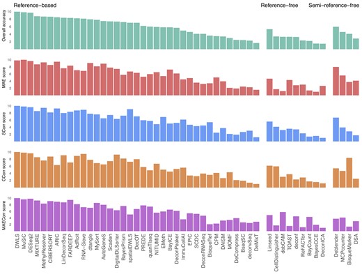
The accuracy scores of the deconvolution methods obtained from the analysis of 30 tissues available on Tabula Sapiens and CELLxGENE. The accuracy is measured by four different metrics: (i) mean absolute error (MAE), (ii) sample-wise Spearman correlation (SCorr), (iii) cell-type-wise Spearman correlation (CCorr) and (iv) mean absolute error between the two sample-pairwise Pearson correlations (MAECorr). Each score ranges from 1 to 10 (the higher the better). The methods are ordered by their overall score, which is the average of the four metrics.
In general, reference-based methods outperform reference-free methods in all accuracy metrics. The scores of reference-based methods are more consistent across the metrics compared to those of reference-free methods. One important note is that the performance of each method varies greatly across tissues. It is also noticeable that in some tissues, including Liver, Lung, Small Intestine and Trachea, most methods consistently have larger MAE than other tissues. Note that these tissues also only have a few cell types (2–4, see Table 1).
We observe that there is no method that has the best scores in all tissues. For the MAE metric, the best three methods are MuSiC, DWLS and DESeq2’s unmix (Supplementary Figure S4). The differences in MAE values of the 10 top methods are small, with the smallest MAE is |$5.7\%$| and the largest MAE is |$7.0\%$| (Supplementary Figure S5). For the SCorr metric, the best three methods are DWLS, MuSiC and DESeq2’s unmix with average correlations of |$81.4\%$|, |$79.5\%$| and |$77.4\%$|, respectively (Supplementary Figures S6 and S7). There is a considerable gap among the top 10 methods with the highest correlation being |$81.4\%$| and the lowest correlation being |$69.5\%$|. The small differences in MAE but large differences in SCorr of the top methods suggests that deconvolution methods are struggling to keep the order of the estimated cell type proportions for cell types that have similar proportions.
The three best methods with CCorr metrics are DWLS, MuSiC and DESeq2’s unmix with average correlations of |$78.7\%$|, |$78.3\%$| and |$77.4\%$|, respectively (Supplementary Figures S8 and S9). The top 10 methods for this metric have a correlation of at least |$71.6\%$|. For the MAECorr metric, the best three methods are DWLS, DESeq2’s unmix, and MuSiC with average MAECorr values of |$12.1\%$|, |$12.8\%$| and |$14.6\%$|, respectively (Supplementary Figures S10 and S11). Top 10 methods for this metric have the MAECorr of at most |$17.7\%$|. We observe that methods that perform well on the former metric can still have a relatively large error in the latter one. Also, the higher scores of MAE and SCorr compared to CCorr and MAECorr suggests that the deconvolution results are more suitable for studying relationships between cell types and phenotypes, rather than relationships among subjects (such as patient segregation), or among cell types. Note that spatialDWLS (DWLS tailored for spatial data) fails to achieve the same performance as DWLS. This is because spatialDWLS is designed to work with fewer cells per sample. Supplementary Figures S4–S9 show that this method works well with small numbers of cell types. This finding is consistent with other benchmarking articles (38,39) when spatialDWLS is among the top performers for 2–6 cell types (38), but does poorly when there are more than ten cell types per spot (39).
Finally, we note that all methods are biased towards certain cell types, i.e. all of them consistently underestimate or overestimate the proportion of specific cell types. To quantify the bias of each method, for a pair of a method and a cell type, we used a paired t-test to compute the significance of the difference between the estimated proportions and the ground truth. For the cell types used in our benchmark, all methods significantly underestimate or overestimate the proportion of at least 10 cell types with absolute mean difference >0.1 (Supplementary Figure S12). The number of cell types with large absolute mean differences can be as high as 42 as for BayesCCE.
Scalability
We measure the scalability of the methods by analyzing datasets with an increasing number of bulk samples (100, 250, 500 and 1000 samples). We assess the scalability of each method by measuring the running time (hours) and memory usage (gigabytes). We first rank the methods based on their average running time and memory usage, assigning lower ranks to methods that consume less computational resources. Similar to the accuracy metrics, we calculate the scalability score by scaling the ranking into the range of [1, 10] to obtain a quantitative score for each method, where lower ranks correspond to higher scores.
Most methods can analyze hundreds to thousands of samples in minutes. Overall, we found that scalability should not be a major concern, as deconvolution methods have linear time complexity with regard to the number of bulk samples, and they use at most 3GB of memory in the process. Even the slowest method, EMeth, can deconvolve 1000 samples in six hours. This is to be expected since many methods spend most time for processing the signature or training the model before estimating the cell type proportions for each individual sample, which can be easily scaled to multiple cores or compute nodes. Methods with high-time complexity are mostly those that perform regression on all (ARIC, DESeq2 and EMeth) use Bayesian methods (BayICE and BayCount), or repeatedly subsampling to optimize the parameters (DWLS).
Another reason that makes scalability to be less of a concern is that the number of bulk samples for deconvolution is limited to the number of subjects in the study cohort, which is usually on the scale of hundreds to thousands of patients. For instance, the majority of human datasets in the GEO database have <200 samples, and two tissues with the largest number of samples in the GDC cancer portal, Lung and Breast, both have only over 1000 samples. The running time and memory usage of each method with different settings of the number of samples are reported in Supplementary Figure S13 and Supplementary Table S3.
Consistency
There are many factors that can influence deconvolution analysis including dropout in single-cell data, noise in bulk and reference data, and random factors in computing the cell type proportions. There are software packages such as Splatter (134) and SymSim (135) that can be used to simulate single-cell data with various characteristics. However, we preferred to generate datasets by sampling real single-cell datasets that already have high dropout rates. Across our experiments, the single-cell data are generated by sampling real single-cell data has dropout rates ranging from 77% to 98% (Supplementary Figure S1). To quantify the robustness of each deconvolution method, we repeatedly add Gaussian noise to the input (bulk and reference data) and measure the consistency of the results. Specifically, for each gene g in both bulk and reference data, we add a small amount of noise following Gaussian distribution |$\mathcal {N}(0,\, \sigma ^{2}_n)$|, where |$\sigma ^{2}_n=0.01\times \sigma ^{2}_g$| where σg is the standard deviation of gene g. For methods that require markers, we randomly remove 5% of the markers for each cell type in each run. Finally, we calculate: (i) the coefficient of variation (standard deviation divided by mean) as the dispersion of the estimated proportions and (ii) the deviation of the correlation with ground truth. The dispersion and standard deviation of correlation for each method are reported in Supplementary Figure S14.
In a similar manner to accuracy and scalability, we rank the method’s consistency by averaging their their dispersion and deviation of the correlation. A lower rank indicates a smaller average dispersion and standard deviation of correlation, reflecting greater consistency in the method. Next, we concert methods ranking into scores between 1 and 10, with higher scores meaning that the methods achieve higher consistency.
There are many factors that can influence deconvolution analysis including noise in bulk and reference data, and random factors in computing the cell type proportions. To quantify the robustness of each deconvolution method, we repeatedly add artificial noise to the input and measure the consistency of the results. Specifically, for each gene g in both bulk and reference data, we add a small amount of noise following Gaussian distribution |$\mathcal {N}(0,\, \sigma ^{2}_n)$|, where |$\sigma ^{2}_n=0.01\times \sigma ^{2}_g$| where σg is the standard deviation of gene g. For methods that require markers, we randomly remove 5% of the markers for each cell type in each run. Finally, we calculate: (i) the coefficient of variation (standard deviation divided by mean) as the dispersion of the estimated proportions and (ii) the deviation of the correlation with ground truth. The dispersion and standard deviation of correlation for each method are reported in Supplementary Figure S14.
We found that a majority of methods are susceptible to noise. Only eight methods have the dispersion smaller than 0.1: AdRoit, dtangle, CPM, MuSic, DecOT, DWLS, ReFACTor and DSA. Some methods even have the dispersion larger than 1 (i.e. standard deviation is greater than mean), indicating that the results of these methods are very unstable. Similarly, 44 out of 48 methods have the standard deviation larger than 0.1, suggesting that the order of the cell type proportions can be easily influenced by noise.
Stability and usability
Method stability and usability play an important role in how well the method is received by the community. While researchers mainly seek to use the most accurate method, installation issues, crashes, poor documentation, fine-tuning many parameters might prevent users from trying or effectively deploying a given method.
Here, we measure method stability by how well the methods finish an analysis without crashing. This metric also reflects the quality of testing that was performed when the method was published. Across all analyses conducted in our benchmarking, we calculate the percentage of successfully completed analyses for each method. The percentage is then scaled to the range between 1 and 10 and rounded up, resulting in the final stability score for each method. With a total of 130 datasets (30 datasets from the accuracy assessment, 20 datasets from the assessment for missing cell types and 80 datasets from the scalability evaluation), we observe that 24 methods occasionally failed to finish some datasets (Supplementary Table S4). Most methods can finish all analyses without crashing. Among the methods tested, only eleven methods have crash rates of more than 10%. These are cellDistinguisher (crash rate of 57%), DeCompress (50%), debCAM (46%), Bseq-SC(28%), spatialDWLS(27%), EMeth(23%), ARIC(23%), DigitalDLSorter (20%), BayCount (17%), DAISM (15%) and AdRoit (13%).
We also quantify the usability of a method based on the quality of the source code, installation, documentation and user-friendliness (Supplementary Tables S5 and S6). Each criterion is scored between 1 and 5 (the higher the better). For each method, we calculate the average score. The scores of all methods are then scaled to the range of [1,10] and rounded to establish the method’s usability score. Most methods are open-source using GPL, MIT or BSD licenses, allowing users to freely download, modify and distribute the source. The exceptions are MySort (Galaxy), DCQ (not available) and CIBERSORT (custom license). It is worth noting that most methods used R and Python, which are free and open-source. Only SMC, BayesCCE and Deblender use Matlab which requires a Matlab license. Methods that are easiest to install are those deposited in official package repositories such as R package repositories (CRAN and Bioconductor) and Python package index (PyPI). However, 36 out of 53 methods are available on GitHub as a package or scripts. Many of these methods have a problematic installation, including missing dependencies or incompatibility with the latest version of the runtime environments. Documentation, tutorials and function manuals are also sometimes of less than ideal quality or not available.
Impact of incomplete reference data
To understand the impact of incomplete reference data, we perform more analysis using data obtained from CELLxGENE. Each tissue from CELLxGENE has 10 cell types or more, which allows us to generate experiments in which there are substantially more cell types in the bulk data than the reference data. In each experiment, we first generate the complete data (reference, bulk, true proportions) and then remove 25% and 50% of cell types from the reference data. We compare the performance of deconvolution methods in three scenarios: (A) the reference data is complete (i.e. no missing cell types), (B) the reference data lacks 25% of cell types and (C) the reference data lacks 50% of cell types. Consistent with previous analyses, we quantify the accuracy of the deconvolution methods using four metrics: (i) mean absolute error (MAE), (ii) sample-wise Spearman correlation (SCorr), (iii) cell-type-wise Spearman correlation (CCorr) and (iv) mean absolute error between the two sample-pairwise Pearson correlations (MAECorr).
Note that for scenarios B and C, the proportions in the ground truth have more cell types than the predicted proportions. To match the predicted cell types with those in the ground truth, we use the Hungarian algorithm (Kuhn–Munkres) (136) implemented in the RcppHungarian R package (137) to perform maximum bipartite matching. This algorithm identifies pairs of cell types by calculating the Pearson distance between each pair of cell types in the ground truth and predicted proportions. Next, the algorithm searches for one-to-one matching that minimizes the total distance. After matching, we compare the values between the ground truth and predicted proportions to calculate the four accuracy metrics (MAE, SCorr, CCorr and MAECorr).
Supplementary Figure S15 shows the accuracy scores in all three scenarios. In general, the accuracy of most methods decreases when the reference is incomplete, but reference-free and semi-reference-free methods perform relatively well. Note that the incomplete reference affects the performance of not only reference-based methods, but also reference-free and semi-reference-free methods because we provide them with the number of cell types in the reference. With 25% of cell types missing (scenario B), the top methods in these two categories (Linseed and Deblender) have scores similar to that of complete data (scenario A). With 50% of cell types missing (scenario B), the performance of these two methods decreases only slightly. However, methods in these two categories are less accurate than top reference-based methods in any scenario.
The reference-based methods are affected the most in case of missing cell types. Compared to scenario A (complete reference), the overall accuracy of top methods in this category drops in scenario B (25% missing) and further decreases in scenario C (50% missing). The performance gaps between the top methods in this category and the rest become smaller when the reference is incomplete (B and C). However, the rankings of reference-based methods are very consistent in all scenarios, with a correlation of 0.96 between A and B, and a correlation of 0.88 between A and C. Seven methods (DWLS, DESeq2’s unmix, MuSiC, CIBERSORT, ARIC, LinDeconSeq and MIXTURE) are ranked in top 10 in all three scenarios, while 13 methods (DWLS, DESeq2’s unmix, MuSiC, CIBERSORT, MethylResolver, ARIC, LinDeconSeq, FARDEEP, MIXTURE, MySort, AdRoit, ImmuCellAI and Scaden) are consistently among the top 15 in all three scenarios.
Practical guidelines and discussions
The number of deconvolution methods has been growing rapidly since the concept was first introduced in 2009 (138). In this article, we present a comprehensive review and evaluation of 53 such methods to assess their methodology, accuracy, scalability, consistency and stability in estimating cell type proportions from mixture bulk data. We also discuss the quality of the implementation, documentation, and user-friendliness of the methods. Our goal is not to only provide a practical guideline for users to select the most suitable method for their analysis, but also to provide a reference for the current stage of the field and for the future development of deconvolution methods. One of the limitations of this paper is that we did not evaluate the methods for the effect of mixing two or more cell types. A researcher that is concerned about this problem should undertake additional benchmarking in order to understand the way various methods cope with this problem.
Guideline for practitioners
Figure 6 presents a general guideline for users to choose deconvolution methods that are most suitable for their data and purpose. The guidelines only include methods that have high accuracy and stability in the technical evaluation, i.e. mean absolute error (MAE) of at most 10%, all correlation metrics (SCorr, CCorr) of at least 60%, and stability of at least 95% (crashing rate of at most 5%). The figure provides the statistics of the selected methods, including all four accuracy metrics (MAE, SCorr, CCorr, MAECorr), running time and memory usage for various input sizes, and method usability (see Supplementary Section S3).
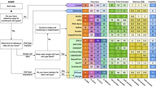
Guideline for selecting suitable methods for cellular deconvolution. The diagram shows the summary statistics of the methods, including their accuracy, running time, memory usage and usability. The accuracy includes four metrics: (i) sample-wise mean absolute error (MAE), (ii) sample-wise Spearman correlation (SCorr), (iii) cell-type-wise Spearman correlation (CCorr) and (iv) mean absolute error between ground-truth and predicted correlation matrices (MAECorr). Note that this diagram only presents the top methods that have their overall score of at least 7, and are the most accurate with correlation metrics of at least 60% and mean absolute error (MAE) of at most 10%. Note that Linseed has SCorr 58% but we include it in the guideline because it is the only reference-free method that has overall score over 7 and MAE less than 10% . The input of all deconvolution methods must include a bulk dataset. Depending on additional input data, the diagram points to suitable software. For example, if one does not have any data that can be used as a reference, then Linseed, which is a reference-free method, may be the optimal choice. However, if one can provide the list of marker genes of the constituent cell types, then Deblender may be a better choice. If more reference data are available, one can choose one of the reference-based methods.
To illustrate how these results can be used to choose the best method for a given application, let us consider a situation in which no reference data is available. Our results suggest that in this case, Linseed might be a good option since it does not require any reference data. However, if possible, we suggest users provide reference data, including the markers, single-cell expression, and expression of reference cell types. This additional information would allow users to improve the accuracy of the deconvolution process. For example, even when users only know the marker genes of the cell types in the tissue, they can apply Deblender, a semi-reference-free method, to deconvolve the data. Such list of marker genes can be easily obtained from the literature or from public databases such as CellMarker (139) and PanglaoDB (140).
An even better situation is when users can provide single-cell expression data with cell type labels of the same tissue as the reference. Such reference data would allow to: (i) identify the markers of known cell types using differential analysis and (ii) generate the signature expression for each cell type. If the true cell type labels of the cells are not available, one can perform supervised or unsupervised learning to segregate cells into different cell types or groups. For supervised learning, one can obtain the markers of potential cell types in the tissues from public databases and then apply classification methods to classify the cells to known cell types For unsupervised learning, one can segregate the cells into cell groups using clustering methods developed for single-cell data. Some methods require cell-type expression as the reference data, which are usually pure bulk expression data or obtained from other studies. This cell-type expression usually contains the expression of only marker genes. In principle, many of these methods can also be run if one can provide a full cell-type expression without filtering out non-marker genes. However, this should only be the last resource since these methods are not designed to handle such a reference.
When performing cellular deconvolution, we recommend users analyze their data using multiple methods and multiple initializations to confirm that they have high confidence in the analysis results. However, each method requires a different runtime environment (i.e. R, Python, Matlab, Shell script) and different input formats, making it difficult to conduct systematic analysis and comparison. In order to address this issue, we provide an R package that can be used as a wrapper to easily run any of these deconvolution methods. Each method is preinstalled in a docker image and will be executed as a container using either a docker or a singularity engine. We note that, for a few methods, users will need to acquire a license to run them. This includes methods implemented in MATLAB (BayesCCE, SMC, Deblender) which is a proprietary programming language, and CIBERSORT whose code needs to be requested from its authors. The list of supported methods can be easily extended by containerizing newly developed tools.
Researchers can also apply the methods in our package to analyze spatial transcriptomics data by treating each spot or location as a bulk sample. For instance, AdRoit consistently ranks among the top-performing methods across various experimental settings, as highlighted in a recent comprehensive review on deconvolution methods for spatial data by Chen et al. (40). MuSiC demonstrates strong performance when evaluated based on the root mean squared error between the predicted proportions and the ground truth, as observed in the comparison of method performance by the authors of CARD (141). Nevertheless, there are two limitations when applying the bulk transcriptome deconvolution methods to spatial transcriptome data. First, these methods do not take into consideration the physical location information from the spatial transcriptomics. For example, the cell-type compositions on neighboring locations contain valuable information for inferring cell-type composition on the location of interests (141). Second, the spatial transcriptomics data contain thousands of spots, thus, it may require substantial time and space complexity to run the methods on this type of data (113) (also see Supplementary Figure S13). We recommend users to consult benchmarking papers for spatial transcriptomics data (38–40).
Outstanding challenges in cellular deconvolution
There are outstanding challenges that need to be addressed to improve the quality of deconvolution results. First, most methods assume that the marker genes are mutually exclusive between cell types. However, this assumption is not always true. For example, in the immune system, the expression of CD4 and CD8 marker genes are not mutually exclusive between CD4+ T cells and CD8+ T cells (142). This phenomenon is more common among subtypes of the same cell type (e.g., Th1, Th2 and Th17 cells of CD4+ T cells), where subtypes share common markers as the marker of the cell type. When this assumption is violated, the deconvolution results can be biased against the cell types that have overlapping markers. Multicollinearity between cell types also leads to unstable results or multiple solutions in cellular deconvolution. This challenge is particularly evident in high-purity mixtures of tumor cells, where deconvolution methods may mistake normal epithelial cells with cancer epithelial cells due to their transcriptional similarities (37). Also, because of the non-overlapping markers, when the bulk expression has a similar expression pattern with the small set of markers of a cell type, the proportion of that cell type might be overestimated. Another factor that contributes to underestimated/overestimated proportions is that the actual number of cell types in the bulk data might be larger than the number of cell types in the signature matrix. Under this situation, the compositions of the cell types that are not in the signature matrix will be distributed to the cell types in the signature matrix, leading to the overestimation.
In addition, current deconvolution methods do not consider the dynamics and interdependence of cells. The measured expression profiles of cells and cell types can be perturbed by many factors, including biological heterogeneity (microenvironment and cell development) and technological variation (sequencing technology, library preparation, etc.). In fact, cell states play an important role in the variability of the expression of cells, and the appearance of a cell type can affect the expression of other cell types. For example, the expression levels of the marker genes in T cells are not only affected by the activation state (activated or resting) of the cells (143), but also by the presence of other cell types, such as macrophages (144). This cell expression dynamics has also been shown in many studies of cell differentiation using single-cell data (145). Other confounding factors such as the different phenotypes between the reference and the bulk samples, batch effects, and technical variations can also affect the deconvolution results. In other words, the ideal reference expression profile needs to: (i) reflect both the dynamic within and between cell types, (ii) match the phenotype of bulk samples and (iii) use the same sequencing platform as used for the bulk sample. Such reference expression profile is difficult to obtain since it requires tremendous efforts to collect the reference data from different mixtures of cell types and different conditions.
Another key challenge for deconvolution is to accurately validate the performance of the methods. Current problems include the difficulty of determining the ground truth of bulk samples for a large number of cell types and tissues. The majority of bulk samples accompanied with cell type compositions are from blood samples obtained from flow cytometry. This introduces bias to the development of deconvolution methods because they overfit to the cell types in blood. Although one can use purified cell lines to generate data for other cell types, datasets generated in vitro usually have a low number of samples and cell types. Using two libraries from the same tissue of the same donor, one for bulk sequencing and another for single-cell sequencing to determine the ground truth, can produce reasonable reference profiles but does not guarantee the reliability of the ground truth. This is because the cell type proportions in the single-cell data are not necessarily the same as those in the bulk data due to tissue dissociation (99,146,147) and other factors. This presents a challenge not only for the validation of deconvolution methods, but also for many research areas that use single-cell profiling.
Data availability
The Tabula Sapiens and CELLxGENE single-cell data used for technical evaluation are deposited on the following Zenodo repositories: https://doi.org/10.5281/zenodo.10687798 (Tabula Sapiens) and https://doi.org/10.5281/zenodo.10688809 (CELLxGENE), respectively. The simulated data are available at https://doi.org/10.5281/zenodo.10891254. Prebuilt docker images are available on Docker Hub at https://hub.docker.com/u/deconvolution. The source files to build the docker images are available at https://doi.org/10.5281/zenodo.10891276. The wrapper to run all methods is available at https://doi.org/10.5281/zenodo.10891290. Scripts to generate the evaluation results are available at https://doi.org/10.5281/zenodo.10891326.
Supplementary data
Supplementary Data are available at NAR Online.
Acknowledgements
This work was partially supported by NSF (grant no. 2343019 and 2203236), NIGMS (grant no. 1R44GM152152-01), and NCI (grant no. 1U01CA274573-01A1). Any opinions, findings, and conclusions or recommendations expressed in this material are those of the authors and do not necessarily reflect the views of any of the funding agencies.
Author contributions: Hung Nguyen and Ha Nguyen reviewed all deconvolution articles and jointly designed the technical evaluation. Duc Tran helped with data processing and implementation. Sorin Draghici helped with technical evaluation and discussion. Tin Nguyen supervised all aspects of the work. All authors jointly wrote the manuscript.
Funding
National Cancer Institute [1U01CA274573-01A1]; National Institute of General Medical Sciences [1R44GM152152-01]; National Science Foundation [2203236, 2343019]. Funding for open access charge: National Science Foundation.
Conflict of interest statement. None declared.
References
Author notes
The first two authors should be regarded as Joint First Authors.

Comments