


Abstract
In many cases, the unprecedented availability of data provided by high-throughput sequencing has shifted the bottleneck from a data availability issue to a data interpretation issue, thus delaying the promised breakthroughs in genetics and precision medicine, for what concerns Human genetics, and phenotype prediction to improve plant adaptation to climate change and resistance to bioagressors, for what concerns plant sciences. In this paper, we propose a novel Genome Interpretation paradigm, which aims at directly modeling the genotype-to-phenotype relationship, and we focus on A. thaliana since it is the best studied model organism in plant genetics. Our model, called Galiana, is the first end-to-end Neural Network (NN) approach following the genomes in/phenotypes out paradigm and it is trained to predict 288 real-valued Arabidopsis thaliana phenotypes from Whole Genome sequencing data. We show that 75 of these phenotypes are predicted with a Pearson correlation ≥0.4, and are mostly related to flowering traits. We show that our end-to-end NN approach achieves better performances and larger phenotype coverage than models predicting single phenotypes from the GWAS-derived known associated genes. Galiana is also fully interpretable, thanks to the Saliency Maps gradient-based approaches. We followed this interpretation approach to identify 36 novel genes that are likely to be associated with flowering traits, finding evidence for 6 of them in the existing literature.
INTRODUCTION
Genome Interpretation (GI) is the umbrella term describing the scientific endeavor towards understanding the genotype-to-phenotype relationship (1,2). Being able to precisely model how the information encoded in our genome leads to the observed phenotypes would indeed constitute a crucial advancement for genetics and molecular biology, and could open a new era for precision medicine (3).
Early efforts in this sense include Genome Wide Association Studies (GWAS) (4) and various attempts at the interpretation of variants in Whole Exome and Genome Sequencing studies (WES, WGS) (5,6). Unfortunately, the loci discovered through GWAS are not causative for the phenotype under consideration (4), as they only are in linkage disequilibrium with the truly causative alleles, and thus offer a quite low resolution for GI. As a result a large part of the heritability of complex diseases is still left unexplained (4,7). Moreover, the power of GWAS markers for the construction of actually predictive Polygenic Risk Scores has been recently disputed (8,9).
On the other hand, WES and WGS studies can theoretically identify every form of genetic variation with respect to a reference genome, and thus this data is much more likely to contain the set of causative variants for the phenotypes under study (5). Notwithstanding the richness of the information contained in this data and the widespread availability of this sequencing technology, the bottleneck has unfortunately only shifted from data availability to data interpretation. In most real-life application, the generally few causative variants for the phenotype of interest are indeed hidden in the plethora of neutral variation regulating normal phenotypic expression and mildly deleterious variants that are associated with other phenotypes, leading to the proverbial needle in the haystack problem. To overcome this issue, bioinformatics methods such as variant-effect predictors (VEP) (10–13) and variant-prioritization tools (VPT) (14–16) have been developed, respectively aiming at determining the functional impact of missense variants and prioritizing the variants that are most likely to be involved in a target phenotype. Although these approaches can be used as building blocks for more comprehensive GI pipelines (15), they have severe conceptual limitations because for example VEP assume perfect Mendelian inheritance and consider only one variant at a time, while VPT can recommend the set of variants that are most likely involved in a phenotype, but do not aim at modeling how these variants influence that phenotype.
In recent years, some methods for Genomic Prediction for plants and animal breeding have been proposed (17), in some cases involving Machine Learning (18,19). Nevertheless, these approaches mostly rely on Single Nucleotide Polymorphism (SNP) markers (similarly to GWAS approaches) and aim at the prediction of relatively few (≤10) phenotypes. A comprehensive ‘end-to-end’ GI approach, able to model the phenotypic expression produced by a given genome, is still currently missing, even though uncovering how the genotype leads to the observed phenotype would be a crucial achievement for genetics.
In this paper, we take a step towards full-fledged GI by attempting the most detailed modeling so far of the genotype-to-phenotype relationship in A. thaliana (20). A. thaliana (AT from now on) is a small flowering plant that belongs to the Brassicaceae family, and it presents several characteristics that made this species the model organism for research in plant genetics and molecular biology. AT is indeed characterized by a small genome (∼125 Mb), a short life cycle, a very efficient transformation method and the availability of a wide range of genetic and molecular resources (including a large collection of mutants) (21). AT is a self-pollinating species, meaning that plants catalogued with the same accession number in (21) sampled in nature are homozygous. These characteristics and the fact that several AT accessions are widely found in nature at very different latitudes (21), made AT an ideal species to study local adaptation to very diverse environments and related phenotypes. Moreover, since the sequencing of its genome in 2000 (22), the amount of available sequencing data, including WGS data (21) and detailed phenotypic annotations (23), greatly increased.
In this paper, we combined the AT WGS data from 1001genomes.org (21) with the corresponding phenotypic annotations from AraPheno (23) and we built what, to the best of our knowledge, is the the first in-silico model aimed at the multi-phenotype interpretation of the AT genome. Our model, called Galiana, is an end-to-end Neural Network that takes as input AT sequencing data and performs a multi-task regression, concurrently predicting 288 real-valued phenotypes describing morphological, structural and developmental traits of AT samples. Galiana is able to predict 75 out of 288 phenotypes with a Pearson correlation greater than 0.4.
Our modeling approach and its results are conceptually different from the previous GWAS-based GI attempts on AT. In particular, Galiana (i) is predictive for each target phenotype instead of providing a purely qualitative analysis and (ii) it is based on WGS data and thus it can directly model the phenotypes from the directly causative variants. Moreover, we show that our end-to-end approach, which takes as input the entire AT genome in the form of a VCF file, outperforms analogous models based on just the known associated genes on 77% of the phenotypes for which it was possible to run this comparison. At the same time, Galiana is able to predict also phenotypes for which no gene associations are already known.
Finally, notwithstanding its complexity, our model is interpretable in the sense that gradient-based methods belonging to the Saliency Maps (24,25) family can be used to investigate how the predictions for each input sample have been computed. In the genetics context, this translates to the ability of identifying the most relevant genes associated to each phenotype, given the trained model. We thus extracted the associated genes for the 75 most reliably predicted phenotypes, and we performed a GO-terms enrichment analysis. We then focused on the flowering-related phenoytpes, which are the most represented class among the best predicted phenotypes, and we showed that Galiana identified 36 novel genes that are likely associated with the flowering traits. Among these 36 putatively associated genes, 6 (17%) have indeed been already characterized for playing a major role in flowering, suggesting a certain degree of reliability in these newly found associations.
MATERIALS AND METHODS
Dataset
From the 1001 AT genomes database (21) we downloaded the WGS data of 1135 AT samples. From AraPheno (23) we downloaded the corresponding phenotypic annotations, consisting of 444 phenotypes from 16 studies. From this set we removed 122 phenotypes and variables coming from a single study, because of their relation to geographic and climatic characteristics of the environment of origin of AT samples. We also removed 34 phenotypes because they had less than 70 observations each, ending up with 288 phenotypes mapped over 1021 AT genomes coming from 46 countries.
The vast majority of these phenotypes are real valued measurements of AT characteristics under certain growth conditions (see (23) for more details). In case repeated measurements have been performed for certain phenotypes, we took the mean of these values as a regression target. A list of the predicted phenotypes and their range of values is shown in Supplementary Table S1. The number of AT samples available for each phenotype is shown in Supplementary Table S2. The number of AT samples available for each country are shown in Supplementary Table S3. The list of the AT samples and their phenotypes used as labels for training is available in Supplementary Table S4. Supplementary Figure S7 shows the distribution of the number of studies targeting each AT sample. Each sample has been used in 5.73 independent studies on average.
Encoding the genetic variability into a ML-understandable feature vectors
We used Annovar to annotate the VCF files containing the variants found in each AT genome. Since no functional annotations are available for AT variants, from Annovar we just retrieved the information regarding the variant type and the kind of genomic region on which it is mapped. Each variant is assigned to one of the following 17 types: (exonic) nonsynonymous, (exonic) non-frameshift insertion, (exonic) non-frameshift deletion, (exonic) stoploss, (exonic) frameshift insertion, (exonic) frameshift deletion, UTR3, UTR5, exonic ncRNA, intronic ncRNA, upstream, downstream, intergenic, intronic, splicing, ncRNA splicing, exonic stopgain.
Following the approach proposed in (1), we encoded the variants by grouping them per-gene, in an attempt to obtain a compact representation of the AT per-sample genetic variability while preserving the information related to the type of variants affecting each gene. We thus represented each of the 27655 genes gi as a 17-dimensional vector containing the occurrences of each type of variants occurring on gi. Each AT sample is thus described by a (Ng = 27655, Fg = 17) tensor representing the number and types of variants mapped on each gene.
The tensor describing each input ends up containing the number of each of the 17 types of variants annotated by Annovar that occur on each gene and is thus similar to an integer-valued histogram, which is not a suitable input for NNs as it might raise numeric issues and convergence problems during the training. We thus scaled the value of each gene by reshaping the vectors used as training from (Ns, Ng = 27 655, Fg = 17) to (Ns × Ng, Fg), applying the standardization z = (x − μ)/σ to each of the 17 dimensions, and restoring the original shape of the tensor. Here, Ns is the number or samples, μ is the mean and σ is the standard deviation.
Encoding the phenotype observations
The 288 phenotypic annotations we obtained after our filtering of the phenotypes provided by AraPheno (23) are real-valued with highly variable value ranges, means and variances (See Supplementary Table S1 for an overview). While trying to predict in a multi-task fashion the 288 phenotypes, this variability will impair the uniform training of the phenotypes, because the losses of the phenotypes with overall higher values will weigh more during training. To overcome this problem, we applied standardization to each phenotype, thus ensuring μ = 0, σ = 1 for all of them, regardless of their original values.
The multi-task neural network model
We build a multi-task Neural Network (NN) model to simultaneously predict multiple phenotypes for each AT sample. The architecture of the NN is shown in Figure 1. Each genome in each AT sample is represented by a (Ng, Fg) tensor containing the histograms encoding the occurrences of the 17 types of variants annotated by Annovar in each gene gi ∈ Ng.
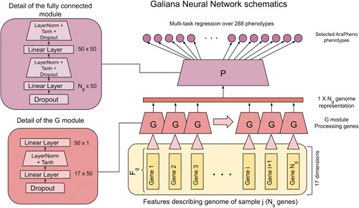
The architecture of Galiana. The (17, N = 27 655) tensorial representation of each genome is used as input. Each 17-dimensional vector representing the gene i is processed by the G module. The iterated applications of the G module produces the (1, 27 655) representation of the mutational load on each gene, which is used as input for the fully connected module, which consists of a FF NN with two layers with 50 neurons each. Finally, the last layer implements the multi-task regression over the 288 real-valued phenotypes.
Similarly to (1), we processed this gene-level information by using the same NN module G for all the genes in all the samples, thus relying on weight sharing in order to minimize the total number of trainable weights in the model (see Figure 1). The G module outputs a single value for each gene, thus compressing the 17 dimensional vectors describing the quantity and quality of the variants mapped on each gene to a scalar value. As shown in the left column of Figure 1, the G module is composed by a Dropout (p = 0.1) module followed by a (17, 50) fully connected layer. The outputs of this layer are processed by a LayerNorm followed by Tanh activation and the final one dimensional output is produced by a (50, 1) output layer.
These per-gene values are then concatenated (see Figure 1) into a (1, Ng = 27655) tensor encoding the compressed information concerning the variants mapped on each gene in the genome of each AT sample. This is then processed by the P module, which is composed by a Dropout layer (p = 0.2) and two fully connected layers (50 neurons each) followed by LayerNorm, Tanh and Dropout (see left panel in Figure 1). The last layer, applied on top of the P module, is a (50, 288) linear layer producing the 288 regression outputs associated with the AT phenotypes.
To optimize the network we used the Adam optimizer, with L2 regularization (λ = 10−5) and MSE loss. We trained the model for 70 epochs using mini-batches composed of 10 AT samples and learning rate equal to 10−3. The goal of the weight sharing in the G module is to reduce as much as possible the complexity of the NN, but the constraints of having i) a minimum of one neuron representing each gene and ii) the 288 outputs sets the final number of trainable parameters to 1456599, which is relatively high with respect to the dataset size. To reduce the effective number of parameters, we relied on the L2 regularization, the various Dropout layers and a relatively small number of training epochs (70).
Since the goal of the network is to compute regressions we used the Tanh as activation functions. To avoid the gradient vanishing problems due to the bounded nature of Tanh, we used a LayerNorm to normalize the values of each layer before applying the activation. We implemented the model using pytorch (26). The code is freely available from our git repository https://bitbucket.org/eddiewrc/galiana/src/master/.
Interpreting the predictions with Saliency Maps
Recent studies (24,25) proposed various gradient-based methods for the instance-based interpretation of NN models. Given a trained NN model M, the forward pass M(xi) for one sample xi at a time is computed, alongside with the gradient ∂Mt(xi)/∂xi of the target output yt = Mt(xi) with respect to the input xi. This allows us to interrogate the model in order to discover which elements in the input feature vector xi are the more relevant for the prediction, since the gradient indicates which input variables needs to be changed the least in order to produce the largest change in the output yt.
In our case, we used the SmoothGrad (24) approach, which consists in repeating the forward/gradient computation steps 50 times for each sample, injecting Gaussian noise sampled from |$\mathcal {N}(\mu =0, \sigma =0.1)$| in the input vector xi at each iteration. This procedure has been shown to reduce the noise in the resulting Saliency Maps (24).
Since Galiana is built to perform a multi-phenotypic regression, we computed SmoothGrad separately for each phenotype. Moreover, since in a regression we are interested in discovering input features that drive the value of the predictions both up and down, we considered the absolute value of the gradient on each input variable.
The goal of our interpretation attempt is to discover which genes are associated with each phenotype. We thus exploited the architecture of our network to simplify this task by computing the SmoothGrad gradients on shared G neurons representing the activation associated to each gene (see Figure 1) instead of computing the gradients on the input features, which are represented as a (17, 27 655) tensor and would thus require some per-gene aggregation of the gradients that might introduce artifacts or noise.
Saliency Maps can sometimes lead to noisy results (24,27), which could be tolerated when applied on image recognition, but could have a much more detrimental effect when the goal is to discover meaningful gene-phenotype associations. To ensure the highest possible consistency of the selected genes, we performed several steps.
First, we computed the SM independently for each phenotype Pj, using the same cross-validation settings used to compute the prediction results. For each phenotype Pj we ranked each gene gi in function of the percentage of AT samples annotated with Pj in which gi appeared among the 100 most important genes. We thus obtained a ranking of the AT genes in function of how many times they have been selected among the 100 most relevant among the entire genome. From this pool of genes, we selected the |$5\%$| of highest ranking genes, which represent the |$5\%$| of the most recurrently selected genes for each Pj.
Since NN training can converge on slightly different optimal solutions in different optimizations, due to the random initialization of the weights, we repeated the cross-validation and the gene-selection procedure 6 times, obtaining 6 pools of the most recurrent |$5\%$| genes for each phenotype Pj. To enforce a consistency of the results and remove the randomness in the selection, for each phenotype we computed an intersection between the selected genes, thus keeping only the genes that appear in the top |$5\%$| ranking in all the six repetitions of the cross-validation. We consider this the final set of genes associated to each phenotype, called FINAL_ASSOC.
GO-terms enrichment analysis computation
To investigate the biological relevance of the genes selected by the SM interpretation approach, we performed a GO-terms enrichment analysis of the genes selected for each phenotype using the standard hypergeometric test described in (28,29). We performed the test on the genes resulting from the intersection of the SM results obtained from the 6 cross-validation runs (FINAL_ASSOC genes).
RESULTS
A Neural Network for the multi-phenotype prediction of AT phenotypes
Galiana is an end-to-end Neural Network model for the in-silico Genome Interpretation (GI) of A. thaliana (AT) genomes. It takes AT genomes as input, in the form of Variant Calling Format (VCF) files and it produces as output 288 real-valued phenotypes associated with each genome.
From 1001genomes.org (21) we retrieved the 1135 AT WGS samples from 46 countries and we annotated them with 444 real-valued AT phenotypes collected in AraPheno (23). These phenotypes describe many different characteristics of AT plants, including structural, developmental and morphological traits, such as plant growth and seed yield related traits or the metabolites concentration in the leaves. After some pre-processing (see Methods for more details), we obtained the final dataset, which encompasses 288 phenotypes mapped on 1021 genomes.
We trained and tested our model with a 5-fold cross-validation and we evaluated the predictions with the Pearson correlation coefficient, the mean absolute error (MAE) and the mean squared error (MSE) with respect to the observed phenotypic values. To the best of our knowledge, this is the first attempt at modeling the direct relation between the genome of an organism and such a wide spectrum of phenotypic aspects, which indeed cover in a very detailed way the spectrum of the AT traits. The full list of phenotypes considered is available in Supplementary Table S1.
Among the 288 phenotypes on which our model is trained, for 75 of them the predictions showed a Pearson r > 0.4 and a Bonferroni-corrected P-value lower than 0.05/288 = 0.000174, which is the minimum reliability threshold we adopted to consider our predictions successful in this study. These 75 phenotypes predicted above the threshold are shown in Supplementary Table S5. From this table we can see that the best predicted phenotypes are related to the growth rate, the flowering time (DTF*, FT*, LD*, SD), seed dormancy and structural characteristics such as leaf number (LN*), fruit number and root length.
To show which kind of phenotypic predictions Galiana can produce, in Figure 2 we show 16 of the 75 phenotypes as scatter plots. In general, we can see that the predictions of flowering-related traits, such as the the days to flowering (DTF, DTF Sweden, Spain, DTFplantingSummer, DTFlocSweden, DTF2, FT16, FT22, LDV, LD, SD, SDV, 0W GH FT) have very high Pearson correlation, indicating that Galiana is able to consistently model their value from the AT genomes. Also seed dormancy (GR21, GR21 warm) and size-related traits (Size Sweden 2009) are shown, with correlations ranging between 0.5 and 0.7.
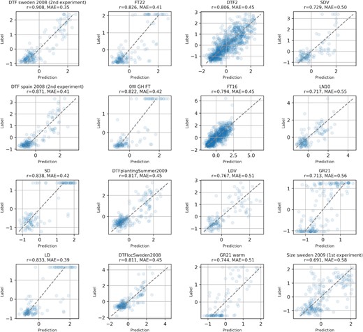
Scatter plots showing the prediction results for 16 of the 75 significantly predicted phenotypes.
Other phenotypes predicted with high Pearson correlation (see Supplementary Table S5) are related to the number of leaves (RL, LN10, LN16, LN22), the number of fruits, the root length (MS-mean Total length, root length days 4, 5), the growth rate, the reproductive growth time (MT GH, LFS GH, LC Duration GH), metabolite content traits (M216T665, M216T666) and stomatal process related traits (delta 13C, delta 13C 261).
Among the most difficult phenotypes to predict, we have the concentration of some elements such as Cu65, Fe57, Ni60, Zn66, P31 and Ca43, which are predicted with a Pearson correlation ≤0.2. Also the flower diameter and the stomata density are some of the hardest phenotypes to predict, with r = 0.14. Various root length and root morphology-related phenotypes (LRLpMRL75, F-mean total length, PF-mean total length, P-mean total length, LRLpMRL0) are predicted with correlations between 0.28 and the selected reliability threshold of 0.4. The list of the phenotypes predicted below the reliability threshold can be found in Supplementary Table S6. The full list of predicted phenotypes, regardless of the threshold, is available in Supplementary Table S7.
In general, it appears that the multi-phenotypic prediction of AT samples from sequencing data is a hard task and that the genotype-to-phenotype relationship on such a wide spectrum of phenotype is indeed driven by highly non-linear mechanisms. For example, Supplementary Figure S6 shows that there is no correlation between the genetic similarity between pairs of AT samples (i, j) and the similarity of their phenotypic profiles (r = 0.080).
Analysis of the synergistic effects between phenotypes during training
From the results shown so far it appears that not all the target phenotypes are predicted with the same reliability. To investigate the causes of the varying performances among phenotypes, we first tried to relate the Pearson correlation of the predictions with the number of samples available as training for each phenotype (see Supplementary Figure S4), finding a relatively low (r = 0.3) correlation. The sheer number of available samples for each phenotype (full list available in Supplementary Table S2) is thus not sufficient to explain the difference in the reliability of the predictions.
On the other hand, Arapheno’s comprehensive list of phenotypes contains many similar traits, or even the same trait measured in slightly different conditions, leading to a certain degree of redundancy among the 288 phenotypes used as prediction targets. To investigate this redundancy, in Supplementary Figure S1 we clustered the phenotypes in function of their similarity. To do so we used a multi-dimensional scaling where the distance between phenotypes (points in the plot) is inversely proportional to their absolute Pearson correlation. Phenotypes that are more similar (correlated) are thus grouped into clusters, and we can indeed see that root, flowering, metabolites concentration and seed-related traits visually cluster together (see Supplementary Figure S1).
In the context of multi-task learning, the intuition behind concurrently training the model to solve multiple problems at once is that if the tasks are chosen in a suitable manner, they could end up positively influence each other during training, giving rise to synergistic effect (30–34). On the other hand, since Galiana is trained simultaneously on all the phenotypes, it is also true that the phenotypes belonging to the largest clusters might be learned more efficiently overall, just because they will have a larger loss weight during training. We investigated this effect, showing that there is indeed a Pearson correlation of 0.79 between the reliability of the predictions for a phenotype P and the number of phenotypes with an absolute value correlation ≥0.5 with P (see Supplementary Figure S3). We obtained similar results (r = 0.69) when we compared the quality of the predictions and the mean absolute correlation of P with all the other phenotypes (see Supplementary Figure S2). This suggests that the phenotypes that are quantified by multiple similar measurements in the dataset (e.g. the flowering trait group) benefit from synergistic effects or are just assigned more relevance during training due to their redundancy, and thus are predicted better.
In relation to this last hypothesis, from Supplementary Figure S1 we can see that this reasoning is not valid for every cluster and class of phenotypes. For example, the two large clusters of root-related phenotypes in the center-bottom and bottom-right corner (TLRL, LRD, LRR, LRL, PF, root, RGR labels) are characterized by extremely poor predictions (Pearson 0 ≤ r ≤ 0.35), with often not even significant P-values (see Supplementary Table S6). To empirically investigate this behavior, we modified the loss function of our NN in order to re-weight the loss function used for each phenotype P with a weight wP which is inversely proportional to the average correlation of P with the other phenotypes (see Supplementary Figure S2). In this way we force the model to level the clustering/correlation-based differences between phenotypes during training, trying to ensure that all the phenotypes are learned at the same pace. Interestingly, all the re-weighting strategies we attempted led to slightly lower performances (i.e. fewer phenotypes predicted above the reliability threshold of Pearson ≥ 0.4), indicating that the sheer similarity among the annotated phenotypes is not likely to be the main reason driving the difference in their prediction performances.
Another possible factor that might produce differences in the maximum achievable accuracy among phenotypes relates to the theoretical upper bound for the accuracy of regressions (35,36). While it is commonly thought that the maximum value that a regression could achieve in terms of Pearson correlation is always 1, in reality the actual upper bound for the predictions might be ≤1 and it depends on both the experimental uncertainty and the variance of the values in the dataset (35,36). Following the approach suggested in (35,36), we computed the theoretical Pearson upper bound for each phenotype and in Supplementary Table S8 we show the ones that have an upper bound <1. The second column in Supplementary Table S8 shows the maximum achievable Pearson correlation given the variance among the repeated experimental measurements and the overall variance among the available annotations (35). Most of these phenotypes represent the concentration of various chemicals in the leaves (e.g. S64, Li7, Na34), thus providing a statistical explanation for the lower prediction accuracy achieved by Galiana on these phenotypes (see Supplementary Tables S6 and S7). For the phenotypes with infrequent repeated measures, it was not possible to compute a meaningful upper bound, and are thus excluded from this analysis.
Also a biological explanation for the differential predictability of the 288 target phenotypes is nevertheless likely to exist. For example, we can hypothesize that flowering-related phenotypes are easier to predict with Galiana due to the strong influence of the geographical origin of the accessions (i.e. the latitude) on these traits. More specifically, it has been shown that flowering time, together with other traits such as seed dormancy, follow a latitudinal cline that does not depend on the population structure gradient (37–39), which usually has a predominant effect on the prediction of phenotypic traits.
Galiana predicts both inter and intra-country phenotype dynamics
In Figure 2, we showed examples of the correlations between the phenotypes and Galiana predictions across the entire dataset, which contains samples from 46 nations. Here we show that Galiana is not just able to predict the ‘average phenotype’ within each nation, but also to predict more subtle phenotype dynamics within each nation. For example Supplementary Table S9 shows the most reliably predicted (Pearson r > 0.4, P-value < 0.000174) phenotypes within the Swedish, Spanish, Italian, German, UK and Russian AT populations. The generally lower number of phenotypes predicted above this threshold is due to the fact that the actual number of the available samples within each specific nation is in many cases significantly lower with respect to the entire dataset, which pools together samples and phenotypic annotations from 46 countries and thus the P-value significance is harder to reach. Supplementary Table S3 shows the amount of samples available for each country, and Supplementary Table S2 shows how many annotated samples are available for each phenotype. Supplementary Figure S5 shows a per-country clustering of the AT genome. Since only Sweden (243 AT samples), Spain (180), US (123), GER (118), Italy (73), UK (69) and Russia (60) have at least 60 annotated samples, we restricted this per-country analysis only to these nations. Below this threshold it becomes indeed more difficult to obtain correlation values that surpass the predictions P-value quality threshold.
In Figure 3, we show the scatter plot of 4 phenotypes for each of the four of the nations with the highest number of AT samples (from the leftmost column to the rightmost, respectively Sweden, Italy, Spain and Russia). We can for example notice that in the Swedish AT population, the concentration of Li7 and S64 are predicted with an acceptable Pearson correlation (first column, r = 0.4 and r = 0.51 respectively), even though these metabolite concentrations are among the most difficult to predict across all the nations (see Supplementary Table S6).
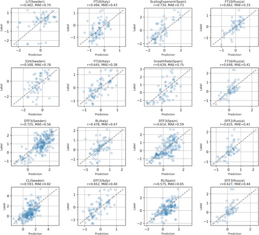
Plots visualizing the predicted correlations for four selected phenotypes while considering only AT samples located in Sweden, Italy, Spain and Russia (represented by the columns, from left to right). This shows that Galiana predicts also intra-nation phenotype dynamics and not only among AT samples belonging to different countries.
In general, the flowering time-related phenotypes such as DTF3 (Sweden), FT10, FT16, DTF2 (Italy), DTF3 (Spain), FT10, FT16, DTF2, DTF3 (Russia) are predicted with high correlation even when data on single nations are taken into account.
Considering the entire genome as input is more effective that using only GWAS-associated genes
Galiana follows an end-to-end prediction approach in which the entire AT genome (composed of 27 500 genes organized in five chromosomes) is used as input for the prediction of the phenotypes. In the multi-task learning philosophy, jointly learning multiple tasks might lead to beneficial effects on the convergence during training and on the generalization ability of the predictor (30–34), due to the synergistic effect of simultaneously learning partially similar tasks and thanks to the informed regularization (30) effect that attending multiple tasks has on the risk of overfitting. Ideally, Galiana should be able to select the genes that are relevant for each phenotype, and benefit during training from the joint learning of groups of synergistic tasks. To empirically verify that this end-to-end genome in, phenotypes out paradigm is truly beneficial for learning, we compared our approach with the results obtained by several phenotype-specific (mono-task) NN predictors trained only on the genes that are known to be associated to each phenotype. To do so we retrieved from araGWAS (40) all the 35 phenotypes with GWAS-associated genes (listed in Supplementary Table S10). For each of these 35 phenotypes Pi we built a dedicated predictor (called GWAS_NNi) that takes as input only the genes that are known to be associated to Pi (see Supplementary Mat. for more details). We thus compared the prediction performances in terms of Pearson correlation, MSA and MSE between these 35 phenotypes predicted by Galiana and GWAS_NNi. The results are shown in Figure 4, which indicates that the whole genome multi-task learning has indeed a positive effect on the predictions for 27 phenotypes out of 35 (77%) using Pearson and for 23 out of 35 (67%) if considering MSE and MAE (bottom panels). We used the paired Wilcoxon test to compare the distributions of the prediction scores, obtaining significant P-values for all the three metrics (top panels), indicating that, notwithstanding the small number of phenotypes for which at least one associated gene was present, the multi-phenotypic prediction approach followed by Galiana outperformed the GWAS_NNi models considering only GWAS-associated genes.
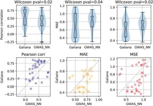
Visual comparison between our multi-phenotypic predictions (Galiana) and the single-phenotype models (GWAS_NNi) based on the known associated genes retrieved from (40). Galiana outperforms the GWAS-based NN 77% of the times on the 35 phenotypes on which the GWAS_NN was applicable.
Moreover, our end-to-end approach, which is agnostic with respect to the genes associated to each phenotype, can attempt the prediction of all the available 288 phenotypes, while the GWAS_NNi models are limited to only the phenotypes for which at least 1 associated gene exists, which is only 35, about half of the phenotypes that Galiana can predict with a Pearson correlation greater than 0.4.
Interpreting the model to discover novel gene-phenotype associations
In order to solve increasingly complex tasks, increasingly complex ML methods are being used and developed, in an attempt to allow the recognition of highly non-linear patterns. Incidentally, this caused the methods to become also more obscure when it comes to understanding the internal decision process that leads to the predictions. To overcome this issue, various methods for interpreting ML models have been developed (24,25,41), with also applications to biological sequence analysis (42) and genetics (1,43).
In this study, we used the SmoothGrad (24) flavor of the Saliency Map (SM) interpretation methods for NN. We interpreted the predictions of the 75 most reliably predicted phenotypes (see Methods for more details). We chose SmoothGrad due to its particular robustness (24,25). While in the image recognition field the SM methods are generally used to highlight the pixels that lead to the predicted class (24), in the context of GI, the goal of the interpretation is to uncover the genes that the model deems the most relevant for the prediction of each phenotype. The intuition behind SM is that once the model M is trained, one sample xi at a time is fed to the NN and the gradient ∂Mt(xi)/∂xi of the target phenotype prediction Pt = Mt(xi) with respect to the input xi is computed. In this way, the model itself assigns gradients to each element of the input feature vector, indicating which input variables need to be changed the least in order to produce the largest change in the predicted phenotype Pt.
We thus assume that the inputs with larger gradient values are the most relevant for the prediction. In the case of Galiana, since we are doing multi-phenotypic regression, for each sample we independently computed the gradient of the inputs with respect to each phenotype t. We also ranked the genes in function of the absolute value of their gradient, since in a regression task we are interested in the signal that drives both up and down the predicted value (see Materials and Methods). We computed the SM using the same 5-fold cross-validation procedure used to compute the prediction results shown so far.
In order to reduce the noise and the possibly spurious genes selected by SmoothGrad, thus increasing the consistency of the resulting gene-phenotype associations, we adopted a few processing steps. First, for each phenotype Pt we ranked the genes gi in function of the percentage of AT samples in which each gi was selected among the 100 most relevant genes. Second, for each phenotype Pt we selected only the highest ranking |$5\%$| of these genes, thus keeping only the genes that are most frequently relevant for the prediction Pt of a certain phenotype t. Third, we repeated the SmoothGrad computation and the processing steps 1 and 2 on six independent cross-validation (CV) runs, obtaining six pools of genes selected for each phenotype. Finally, for each phenotype we computed the intersection between the results of the six CVs, obtaining the final set of genes associated to each phenotype, which is thus formed by only the |$5\%$| of most frequently highest ranked genes genes that appeared in all the CVs. See Methods for more details about this procedure. The genes selected for each phenotype are shown in Supplementary Material S1.
GO-term enrichment analysis of the most relevant genes suggest novel gene-phenotype associations
To investigate the biological relevance of the genes selected with SmoothGrad on the 75 phenotypes considered, we ran a GO-term enrichment analysis on these sets of genes, following the approach adopted in (28,29) (see Methods for more details). This analysis reveals that 59 out of 75 phenotypes presented significantly enriched GO-terms. The GO-terms associated with each phenotype are shown in Supplementary Material S2.
Since many of the most reliably predicted phenotypes are related to flowering (i.e. Days To Flowering (DTF*) phenotypes), we performed a specific analysis using the genes associated to these phenotypes, based on existing literature. In particular, we focused on two studies (44,45) in which the authors measured several flowering traits, together with non-flowering phenotypes. In (44) the authors grew hundreds of accessions in controlled growth chambers that simulate northern and southern European climates (including photoperiod). In the second study (45), the authors measured several physiological parameters and phenotypes on 936 accessions from the 1001 Genomes Consortium (21), grown in controlled conditions.
We then identified the genes associated to the enriched GO-terms exclusively in DTF* phenotypes, separately for each study. Supplementary Table S11 summarizes the 36 genes identified with this analysis and specific to flowering phenotypes for each study. For each gene, we included a description of the related pathway and if the genes were already described for having a role in flowering. Among the pathways associated with the 36 genes identified with this analysis, the most represented were associated to primary and specialized metabolism (seven genes, including terpenes, carotenoids, amino acids and lipids), cell wall (six genes) and cell cycle (three genes).
It is worth noting that two genes identified were in common between the two studies. The first is BBR2a, encoding a spliceosome protein in eukaryotes that affects flowering time by regulating Flowering Locus C splicing (46). The second common gene was Nitrate Transporter 1.6 (NRT1.6), encoding for a nitrate transporter (47) that was never described as flowering time regulator.
DISCUSSION
In this paper, we propose what is, to the best of our knowledge, the first end-to-end multi-phenotype attempt at the Genome Interpretation (GI) of Arabidopsis thaliana (AT). Our model, called Galiana, takes AT genomes as input, in the form of VCF files and concurrently attempts the regression of 288 real-valued phenotypes. 75 of these phenotypes are predicted with a Pearson correlation greater than 0.4.
From the results obtained from Galiana it emerges that the phenotypes related to flowering are generally easier to predict, with very high correlations. In the context of such a heavy multi-task prediction problem, involving hundreds of phenotypes, it is not trivial to determine how each task interacts with the others in terms of synergistic and antagonistic effects (30) during training. We tried to investigate the reasons for the differential accuracy obtained on different tasks by re-weighting the loss function, by considering the redundancy introduced by the presence of correlated phenotypes, or by analyzing the intrinsic prediction upper bound reachable with the data, without finding conclusive explanations. Our main hypothesis for what regards flowering traits is that they are mainly related to the latitude (37,38) and are less influenced by the population stratification.
Another crucial aspect of our approach is that, notwithstanding its complexity, Galiana is not a black box model, since it is interpretable with gradient-based methods from the Saliency Maps (24) family. We used this interpretation approach to determine which genes our model deemed more relevant for the prediction of each of the 75 best predicted phenotypes, and we performed a GO-terms enrichment analysis on them. This analysis identified 36 putative flowering-related genes, and further investigations showed that some of them (17%) were already known to be involved in flowering in literature.
The development of end-to-end GI approaches which follow the genomes in, phenotypes out paradigm and thus directly attempt the modeling of the genotype-to-phenotype relationship, are, in our opinion, crucial for further achievements in genetics and precision medicine. High-throughput sequencing came indeed years ago with great promises, but shifted instead the bottleneck from data availability to data interpretation. Nowadays, thanks to the recent democratization of the access to advanced Machine Learning tools in the form of flexible Neural Network libraries (i.e. Pytorch, TensorFlow), ad-hoc methods can be devised to process data with non-conventional structure, such as genomes and exomes, carefully addressing, if necessary, the limited sample size by reducing the actual and effective numbers of parameters (1) or approaching big-data size datasets scalability issues thanks to mini-batching and parallelization on GPUs.
SUPPLEMENTARY DATA
Supplementary Data are available at NAR Online.
ACKNOWLEDGEMENTS
D.R. is grateful to Anna Laura Mascagni, Nora Verplaetse, Adam Arany and Gabriele Orlando for the constructive discussion. D.R. is funded by a FWO post-doctoral fellowship.
FUNDING
Fonds Wetenschappelijk Onderzoek. Funding for open access charge: KU Leuven.
Conflict of interest statement. None declared.

Comments