


Abstract
Ortholog identification is a crucial first step in comparative genomics. Here, we present a rapid method of ortholog grouping which is effective enough to allow the comparison of many genomes simultaneously. The method takes as input all-against-all similarity data and classifies genes based on the traditional hierarchical clustering algorithm UPGMA. In the course of clustering, the method detects domain fusion or fission events, and splits clusters into domains if required. The subsequent procedure splits the resulting trees such that intra-species paralogous genes are divided into different groups so as to create plausible orthologous groups. As a result, the procedure can split genes into the domains minimally required for ortholog grouping. The procedure, named DomClust, was tested using the COG database as a reference. When comparing several clustering algorithms combined with the conventional bidirectional best-hit (BBH) criterion, we found that our method generally showed better agreement with the COG classification. By comparing the clustering results generated from datasets of different releases, we also found that our method showed relatively good stability in comparison to the BBH-based methods.
INTRODUCTION
Because of the rapid accumulation of data from various high-throughput technologies, comprehensive gene or protein classification is one of the central issues in bioinformatics ( 1 , 2 ). Although classification schemes based on functional roles, molecular interactions or reaction networks have recently become of increasing interest, classification schemes based on sequence or structural similarities are still of fundamental importance. Especially, the accumulation of complete genomes enhances the need for large-scale sequence comparison in light of comparative genomics.
To date, many schemes have been developed to classify proteins into homologous groups, or families. While motifs or profiles that characterize families are helpful for putting the existing knowledge to use ( 3 , 4 ), most of the automated schemes use some clustering techniques applied to precomputed pairwise similarities ( 5 – 11 ). Typically, the focus of these researches has been on either the grouping of weakly similar homologs, or the identification of the building blocks of proteins, termed domains, whose combinations generates the variety of naturally existing proteins.
On the other hand, it has long been recognized that orthology, a kind of homology derived from speciation, should be distinguished from paralogy, a kind of homology derived from duplication ( 12 ). The problem of distinguishing orthologs from paralogs has been formulated as a problem of fitting a gene tree to a species tree ( 13 , 14 ). Recently, the importance of ortholog identification has been widely recognized in the context of comparative genomics. Ortholog identification is crucial for function prediction, since gene functions are typically conserved between orthologs, whereas paralogs can share similar but different functions. Especially, exhaustive ortholog classification is an essential first step in the recently proposed methods of inferring functional linkages between proteins, such as the phylogenetic profile method ( 15 ), the domain fusion method ( 16 , 17 ) and the gene neighborhood method ( 18 ) [reviewed in ( 19 , 20 )]. Phylogenetic profiles can also be used to predict more specific functions when phenotypic traits of each organism are available ( 21 ).
Despite its importance, however, a scheme for large-scale ortholog grouping for multiple genome comparison is yet to be established. The conventional approach to the identification of orthologs between two genomes is the so-called bidirectional best-hit (BBH) criterion, where two genes, a and b , in the genomes A and B , respectively, are considered to be orthologs if a is the best-hit of b in genome A and vice versa. For three or more genomes, orthologous groups can be constructed by extending the BBH relationships with a clustering algorithm. The Clusters of Orthologous Groups (COGs) Database, a widely used curated database for ortholog grouping, was constructed basically through this approach ( 22 ). However, ortholog grouping is not a simple task; the overall COG construction process has included additional complex procedures such as the addition of species-specific paralogs, the splitting of proteins into multiple domains if required, as well as other case-by-case manual modifications ( 23 ). Although several methods have been developed recently to solve some aspects of the ortholog identification problem ( 24 – 31 ), none of them is suitable for any large-scale exhaustive classification comparable to COGs.
Here, we present an efficient algorithm for clustering many protein sequences at the domain level. Our algorithm, DomClust, which was originally developed for our comparative microbial genome database (MBGD) ( 32 ), is a natural extension of the traditional hierarchical clustering algorithm and is suitable for splitting genes into the domains minimally required for ortholog grouping.
MATERIALS AND METHODS
Calculation of sequence similarities
Our procedure takes the results as input of all-against-all pairwise protein sequence comparison containing similarity scores and the beginning and ending positions of the aligned segments. We use the following notations: sim( a , b ) = (score( a , b ), aliab , aliba ) is the similarity relationship between the sequences a and b , where score( a , b ) is the score between a and b and aliab = [ from , to ] is the segment on a that is locally aligned against b . We use square brackets to represent a segment and aliab.fr and aliab.to to refer to the individual endpoints.
Basically any sequence alignment program can be used, but here we used the following protocol: for each significant match found by the BLASTP program ( 33 ) with an adjusted E -value of ≤0.001, rigorous local alignment ( 34 ) was calculated using the JTT PAM250 scoring matrix ( 35 ). Here, we fixed the search space size to 10 9 for every BLASTP search, and the resulting E -value was further adjusted with E × lqls × 10 −5 , where lq and ls are the lengths of the query and the subject sequences, respectively; this adjustment favors global matches between short sequences to short local matches between long sequences.
For measuring relatedness, either the similarity score or the distance can be used. While distance is generally more suitable for evolutionary analysis, similarity is a more appropriate measure of local alignment. Here, we used similarity.
Hierarchical clustering as graph contraction
The above data are used to construct a similarity graph, G = ( S , H ), where S is the set of protein sequences (vertices) and H is the set of homologous relationships (edges). Our clustering procedure is basically a successive contraction of this graph ( Figure 1 ) by the traditional hierarchical clustering method known as the unweighted pair-group method using arithmetic averages (UPGMA) ( 36 ). In each iteration, the procedure takes the best similarity edge, say sim( s1 , s2 ), and replaces the vertices s1 and s2 with a new vertex, sM , representing the merged cluster. In addition, for each vertex s3 ∈ S − { s1 , s2 }, it also replaces the edges sim( s1 , s3 ) and sim( s2 , s3 ) with sim( sM , s3 ), assigning score score( sM , s3 ) = avg 12 [score( s1 , s3 ), score( s2 , s3 ,)], where avg AB ( x A , x B ) ≡ ( x A | A | + x B | B |)/(|A| + | B |) is the group-average function for the quantity x , where | A | denotes the cardinality of the set A . The procedure is repeated until the best score becomes worse than the given cutoff, c .
While the usual UPGMA requires a complete similarity matrix, many edges are actually missing in our similarity graph G , because we consider only significant similarities. Thus, for each iteration with the best edge sim( s1 , s2 ), we must consider only a set of vertices S ( s1 , s2 ) ≡ { s3 | sim( s1 , s3 ) ∈ H ∨ sim( s2 , s3 ) ∈ H }. When one of the two edges is missing, say sim( s1 , s3 ) ∉ H , we assign a fixed score (parameter), m < c , to score( s1 , s3 ) for calculating the average ( Figure 1 ). While maintaining the algorithmic logic, this modification reduces the computational cost of UPGMA from O(| S | 2 ) to O(| H |). Hereafter, we call this simple method ‘gUPGMA’ to distinguish it from the normal UPGMA, where the ‘g’ stands for ‘graphical’ or ‘gap-filling’.
Note that the parameter m combined with the cutoff c can control the granularity of the clustering: m → c approaches the single linkage method, while m →−∞ approaches the complete linkage method. Through a validation test with the COG database as a reference (see below), we found that better results are obtained when m is close to c (data no shown). We set m = 0.95 c throughout the present work. See Supplementary Table S1 for list of parameters used in this work.
Domain splitting: an overview
An exhaustive sequence comparison often reveals a number of domain fusion or fission events ( 37 ). Although such events often provide valuable information for predicting functional linkage ( 16 , 17 ), they complicate the sequence grouping task. To treat these events, we added a process for domain splitting to the basic procedure outlined above ( Figure 2 ). In each iteration with the best edge sim( s1 , s2 ), a merged vertex was split into at most five vertices according to the aligned segment of the best scoring edge: the aligned segment itself and the left and right overhangs on either of the sequences (or clusters); we denoted them sM , s L 1 , s L 2 , s R 1 and s R 2 . For each s3 ∈ S ( s1 , s2 ), the edges sim( s1 , s3 ) and sim( s2 , s3 ) were reconnected to one or more of the new segments, say sM , and the information in these edges, say sim( sM , s3 ) = (score( sM , s3 ), aliM3 , ali3M ), was updated appropriately, by averaging the alignment lengths as well as the scores over all of the relationships included in the merged edges.
Figure 2 shows a simplified example, which contains clusters constituted from six domains, A–F, each of which is 100 residues long. One can easily validate this artificial example, since all alignment boundaries are simply equivalent to the domain boundaries, but this assumption generally does not hold in real cases. For practical implementation, it is necessary to answer the following questions: (i) how do we determine the exact positions to be split on the sequences s1 and s2 , and (ii) how do we update the information in the edges sim( s1 , s3 ) and sim( s2 , s3 ) for each s3 ∈ S ( s1 , s2 )?
The resulting structure is a directed acyclic graph representing overlapping trees, as shown in Figure 2C ; it is further processed for orthologous grouping (see below).
Some concepts: segment overlap, position mapping and alignment consistency
Before describing the procedure precisely, we will introduce some definitions. Let | a | denote the length of the segment a , i.e. | a | = a . to − a . fr + 1. For the two segments a and b , a ∪ b = [min( a . fr , b . fr ), max( a . to , b . to )] and a ∩ b = [max( a.fr,b.fr ), min( a.to,b.to )]; we define [ p,q ] = φ if p > q . The segments a and b are overlapped if | a ∩ b | ≥ Lov ; we denote this by the predicate overlap( a,b ). We also introduce a partial order, ≺, between non-overlapping segments: a ≺ b if a.to < b.fr + Lov . Here, the minimum overlap length, Lov , between the segments a and b is determined by Lov ( a,b ) = min{ rovl min(| a |,| b |), max( lmin , rov2 max(| a |,| b |))} with three parameters, 0 < rov2 < rov1 < 1 and lmin . We set ( rov1 , rov2 , lmin ) = (0.6, 0.3, 50).
In gUPGMA, we consider the three sequences s1 , s2 and s3 at once. Although we usually assume that all pairwise alignments between them are embedded in a common multiple alignment, sometimes this assumption does not hold (especially when there is an internal repetitive structure). To test this, we checked the equivalency of the overlapping patterns between the two segment pairs: { ali31 , ali32 } on s3 and { ali13 , T12 ( ali23 )} on s1 ; we denote this by the predicate consistent( s1 , s2 , s3 ). An overlapping pattern is defined by the order of the four endpoints of the segment pair along each sequence. There are 13 possible patterns, among which we defined an equivalency allowing some flexibility (see Supplementary Figure S1).
Determination of domain boundaries
We must determine up to four boundaries, i.e. the left and right boundaries on the sequences s1 and s2 ; we denote them
We will now focus on the boundary, b R 1 . Starting from the initial boundary,
On the other hand, if there is a s3 ∈ S ( s1 , s2 ) satisfying the following conditions (Condition II; Figure 3B ), we should split the sequence: (i) ali12 ≺ ali13 but not ali21 ≺ ali23 (typically sim( s3 , s2 ) ∉ H , but domain swapping or repetitive structures may yield other patterns), (ii) | ali31 | ≥ rcov | s3 | with a coverage parameter, 0 ≤ rcov ≤ 1 and (iii) score( s1 , s3 ) ≥ csplit with another cutoff score, csplit ≥ c . Only the first condition is essential, which suggests that ali13 and ali12 belong to different domains, while the other conditions are useful to prevent spurious splits from arising when the similarity of ali13 is too weak for an orthologous match.
Let SII ⊂ S ( s1 , s2 ) be a set of s3 satisfying Condition II. We split the sequence at
Finally the segment sM is constructed by merging the segments B1 and B2 ( Figure 3C ). More precisely, it consists of three parts: the aligned segment with the length lMM = avg 12 (| ali12 |,| ali21 |) and the left and right unaligned segments with the lengths
Updating the alignment information
Next, the alignment information between each s3 ∈ S ( s1 , s2 ) and each new segment ( sM , s L 1 , etc.) is updated ( Figure 3C ). The procedure is rather straightforward, although somewhat tedious. Here, we briefly list the key points:
Determine the domain boundaries on s3 (denoted by
\( {B}_{3}=\left[{b}_{{\hbox{ L }}_{3}},{b}_{{\hbox{ R }}_{3}}\right] \)). If consistent( s1 , s2 , s3 ) holds, set B3 = avg 12 ( T31 ( B1 ), T32 ( B2 )), but here we consider only the boundaries that are actually split. Otherwise, prioritize the sequence with better scoring alignment. For example, when score( s1 , s3 ) > score( s2 , s3 ), then B3 = T31 ( B1 ).Determine the endpoints of the alignment between s3 and sM . If consistent( s1 , s2 , s3 ) holds, then merge the two alignments to construct the new alignment with aliM3 = ( TM1 ( ali13 ) ∪ TM2 ( ali23 )) ∩ [1,| sM |] and
\( al{i}_{3\hbox{ M }}=\left(al{i}_{31}\cup al{i}_{32}\right)\cap [{b}_{{\hbox{ L }}_{3}},{b}_{{\hbox{ R }}_{3}}] \). Otherwise, take the alignment with the better score for the new alignment. For example, when score( s1 , s3 ) > score( s2 , s3 ), then aliM3 = TM1 ( ali13 ) ∩ [1,| sM |] and\( al{i}_{3\hbox{ M }}=al{i}_{31}\cap [{b}_{{\hbox{ L }}_{3}},{b}_{{\hbox{ R }}_{3}}] \)(this includes the case sim( s3 , s2 ) ∉ H ).Determine the endpoints of the other alignments. For example, the alignment between s3 and
\( {s}_{{\hbox{ L }}_{1}} \)is given by\( al{i}_{{\hbox{ L }}_{1}3}=al{i}_{13}\cap [1,{b}_{{\hbox{ L }}_{1}}-1] \)and\( al{i}_{3{\hbox{ L }}_{1}}=al{i}_{31}\cap [1,{b}_{{\hbox{ L }}_{3}}-1] \), and the alignment between s3 and\( {s}_{{\hbox{ R }}_{1}} \)is given by\( {\mathrm{ali}}_{{\hbox{ R }}_{1}3}=(al{i}_{13}\cap [{b}_{{\hbox{ R }}_{1}}+1,|{s}_{1}\left|\right])-{b}_{{\hbox{ R }}_{1}} \)(subtraction means translation) and\( al{i}_{3{\hbox{ R }}_{1}}=al{i}_{31}\cap [{b}_{{\hbox{ R }}_{3}}+1,\left|{s}_{3}\right|] \).Assign a score to each new alignment. As described previously, score( sM , s3 ) = avg 12 (score( s1 , s3 ),score( s2 , s3 )), where the missing edges are assigned the score m ; on the other hand,
\( \hbox{ score }({s}_{{\hbox{ L }}_{1}},{s}_{3})=\hbox{ score }({s}_{1},{s}_{3}). \)Do not split the score even when the alignment is split into multiple domains.
Phylogenetic-tree cutting
In the structure shown in Figure 2C , one can identify the clusters of homologous domains by traversing it from top to bottom. Also, one can trace the domain-splitting history of each gene by traversing it in reverse direction. One can split genes into the domains minimally required for ortholog grouping by specifying a set of internal nodes as roots.
To do this, we can fit the gene tree into the species tree ( 13 , 14 ) if we can safely assume that there are no horizontal transfers and know both the true gene tree and the true species tree. However, this assumption does not hold in practice, especially in microbial genomes, where a substantial number of horizontal transfers have occurred. Here, we took a simpler but more practical approach: each root node is recursively cut until the two clusters merged at that node share no or few intra-species paralogous genes ( Figure 4A ). More precisely, a root node with two child nodes, A and B , is cut when | Ph ( A ) ∩ Ph ( B )|/min(| Ph ( A )|,| Ph ( B )|) > p with a given cutoff parameter, p , where Ph ( A ) denotes the set of species contained in cluster A (phylogenetic pattern). Strictly speaking, the parameter p must be 0 according to the definition of orthologs, but actually we found that relaxed conditions, around p = 0.5, often generated a more plausible classification. Here, one can incorporate taxonomic relations by counting closely related species only once. In the validation test described below, we adopted this strategy using the set of related species that are assigned the same code in the COG database (see Supplementary Table S2).
After the set of root nodes is determined, the domain boundaries on each sequence are determined by mapping the boundary positions stored in each internal node on to its leaf nodes by applying the mapping functions T1M and T2M recursively.
Rejoining adjacent domains
Sometimes, the tree-cutting procedure violates the domain-splitting criteria given above. Therefore, the program reexamines the criteria for each adjacent pair of domains in the final step: two adjacent clusters are rejoined when (i) all members in one of the clusters are included in the other, and (ii) the average length of the included cluster is shorter than Lmax . We also considered more aggressive rejoining at the final step: the two clusters A and B are joined when either of the following conditions is satisfied ( Figure 4B ): (i) |adj( A , B )| ≥ radj1 max(| A |,| B |), where adj( A , B ) is the set of adjacent segments belonging to the clusters A and B , or (ii) |adj( A , B )| ≥ radj2 min(| A |,| B |) and the average length of the smaller group is shorter than Lmax ; the latter is a relaxed version of the above original criteria. Here we considered two parameters, 0 ≤ radj1 ≤ radj2 ≤ 1, and found the best values through the COG recovery test described below. This procedure could improve the clustering quality, since split genes found only in one or a few genomes often have abnormal split points, which are unlikely to correspond to meaningful domain boundaries.
Validation test
Our program, DomClust, was implemented in the C programming language. The program was validated using the COG database ( http://www.ncbi.nlm.nih.gov/COG/ ) as a reference. Here we mainly used the 2002 update of the COG database ( 23 ) (referred to as ‘COG02’; 43 genomes, 104 094 sequences, 3307 COGs) but we also used the 2003 update of the COG database ( 38 ) (referred to as ‘COG03’; 66 genomes, 185 898 sequences, 4873 COGs) for comparison. Orthologous groups were reconstructed from the set of sequences in order to create the COGs, which were obtained from the COG web site. Throughout the work, as the original definition of a COG, we considered only orthologous groups comprising genes of at least three phylogenetically distinct organisms (defined by Supplementary Table S2). After eliminating entries that did not satisfy this condition, we retained 3192 COGs in the COG02 set. From this set, we further eliminated groups containing too many paralogs to be considered orthologous groups, and groups conserved in only a few species, which are generally biased and less interesting. For this, we defined a ‘well-defined orthologous group’ (WDOG) somewhat arbitrarily as a group G such that | G |/| Ph ( G )| ≤ 2 and | Ph ( G )| ≥ 5. We extracted 2360 WDOGs.
To evaluate the agreement between the two grouping systems, we first identified a set of corresponding group pairs; for each reference (COG) group, the best compatible group was selected from the target groups. The compatibility between the reference ( R ) and the target ( T ) groups was evaluated using Jaccard's coefficient | R ∧ T | / (| R | + | T | − | R ∧ T |), where R ∧ T denotes a set of segment pairs overlapping between R and T . Here, we considered that the segments a and b are overlapped if | a ∩ b |/max(| a |,| b |) > 0.5. After the set of corresponding group pairs was identified, the total agreement was evaluated by the number of matching group pairs (MGPs). For this, we introduced the following MGPs: an exact MGP is a group pair satisfying | R ∧ T | = | R | = | T |, a phylo-MGP is a group pair satisfying | Ph ( R ∧ T )| = | Ph ( R )| = | Ph ( T )| and | R | ≥ | T |, and a m %-MGP is a group pair satisfying | R ∧ T |/| R | ≥ m /100 and | R ∧ T |/| T | ≥ m /100. Let M Ex , M Ph , M80 and M60 be the number of exact, phylo-, 80%-, 60%-MGPs, respectively. The total agreement was evaluated by MTot = M Ex + M Ph + M80 + M60 . Note that there are overlaps between the various types of MGP, e.g. an exact MGP is also any other type of MGP, and therefore is weighted 4 times as much as a proper 60%-MGP.
For the purpose of comparison, we also tested the following clustering methods: (i) single linkage clustering (SLink), (ii) ‘triangular linkage clustering’ (TriLink), which is our implementation of the original method described in the COG paper ( 22 ) and consists in the merging of triangles in the graph of the best hits when they share the same side and (iii) the TribeMCL algorithm ( 9 ) (the program available at http://micans.org/mcl ), which uses the equilibrium probabilities of a Markov chain defined on the similarity graph for evaluating transitive similarities, a method recently applied to the ortholog grouping problem ( 30 ).
For these methods, the BBH relationships were used as input. Here, we used a relaxed criterion: a gene pair ( a , b ) of the genomes A and B is considered to be in a BBH relationship when the genes satisfy score( a , b ) ≥ rBH max {max y ∈ B [score( a , y )],max x ∈ A [score( b , x )]}, with one parameter, 0 ≤ rBH ≤ 1 ( r BH = 1 corresponds to the rigorous BBH). Intra-species homologs were also included when a gene pair ( a , b ) of the genome A satisfied score( a , b ) ≥ rBH max {max x ∈ G − A [score( a , x )],max x ∈ G − A [score( b , x )]}, where G – A denotes all genomes except A . In addition, we also prepared BBH relationships from which alignments with low coverage, defined as max(| ali12 |/| s1 |,| ali21 |/| s2 |) < rcov , were filtered out. During the evaluation, we systematically changed the parameters r BH and rcov together with the score cutoff c (for SLink and TriLink) or the inflation parameter I (for TribeMCL) to find the parameter set that gives the best MTot . On the other hand, all similarity relationships were used in DomClust, since the algorithm already includes such best-hit-first criteria.
Stability of the clustering methods
We evaluated the stability of the clustering methods by comparing two sets of clusters created from two different datasets, COG02 (old) and COG03 (new). For each method, the same parameters as those selected above (i.e. those giving the best MTot for the COG02 set) were used. After clustering, sequences only in the new dataset were eliminated. In the comparison, we examined which new clusters the members of each old cluster belonged to, and classified each old cluster ( Cold ) into the following six categories: (i) unchanged: there is a unique new cluster that consists of the same members as Cold ; (ii) group-merged: Cold is merged with other old clusters into a new cluster; (iii) group-divided: Cold is divided into multiple new clusters, each of which contain no member of the other old clusters; (iv) domain-merged: similar to group-merged, but allowing different domains (usually adjacent to one another) to fuse into one; (v) domain-divided: similar to group-divided, but allowing splits of a sequence into multiple domains; (vi) others, including more complex cases. We considered the ratio of ‘unchanged’ clusters as an indication of stability. See Supplementary data for the precise definition.
RESULTS
DomClust took about a minute or more to classify the entire COG02 dataset (| H | = 3.5 × 10 6 ) on a 2.4 GHz Xeon machine. This was more than four times faster than TribeMCL with BBH relationships when using the selected set of parameters, even though TribeMCL used a smaller input ( Table 1 ). DomClust has been available on the MBGD server ( http://mbgd.genome.ad.jp/ ) ( 32 ), on which there are more than 200 classified microbial genomes (the DomClust program itself is available at http://mbgd.genome.ad.jp/domclust/ ), but here we focused on the validation of the method using this smaller dataset. At first, as an example of DomClust classification containing domain fusion or fission events, we show the orthologous groups of RNA polymerase beta (RpoB) and beta' (RpoC) subunits ( Figure 5 ). These subunits are fused into one gene in the genomes of two strains of Helicobacter pylori , 26695 (Hpy) and J99 (jHp), while in most archaea, each subunit is further divided into two genes. The history of domain splitting can be traced by traversing the tree in a bottom-up manner ( Figure 5A ): the algorithm first joined the fused genes of Hpy and jHp, and then it divided the cluster into two domains when joining the cluster with the RpoC ortholog of the Campylobacter jejuni (Cje) genome; the remainder domain was subsequently joined with the RpoB ortholog of Cje. By repeating this procedure, DomClust finally identified five orthologous domains ( Figure 5B ).
Evaluation of the clustering methods: the COG recovery test
To evaluate the DomClust algorithm, we performed COG recovery tests using as a reference the set of 2360 WDOGs from the COG02 dataset. First, we performed extensive tests to determine the parameters giving the best agreement with the COG, according to the total agreement value, MTot (Supplementary Table S1). Next, we compared the results with those of the other clustering methods (SLink, TriLink and TribeMCL) applied to the BBH similarity data ( Table 2 and Figure 6 ). For each method, the best parameter set was again selected using the agreement value MTot ( Table 2 ). In addition, we also tested the DomClust algorithm without a domain-splitting procedure, i.e. gUPGMA with the phylogenetic-tree cutting procedure (designated simply as gUPGMA).
DomClust recovered 1060 WDOGs (44.9%) exactly and 1429 WDOGs (60.6%) as phylo-MGPs. These values were greater than those of the other methods ( Figure 6 ). The resulting order of MTot values was SLink (4296) < TriLink (4702) < TribeMCL (5638) < gUPGMA (5827) < DomClust (6176). Note that the TriLink method taken from the original COG construction protocol did not recover the COG groups well, suggesting that the actual COG construction process was far more complex.
We tested the significance of the differences between the methods adjacent in the above inequality with the sign test, where the numbers of entries that showed better/worse agreement were counted, and the P- value was calculated using binomial distribution with a success probability of 0.5. As a result, we found all the differences highly significant ( P < 10 −10 ), except the difference between TribeMCL and gUPGMA, which was only marginally significant ( P = 0.004) (see Supplementary Figure S2). The performance superiority of DomClust over gUPGMA indicates that the domain-splitting procedure was indeed effective. The difference between TribeMCL and gUPGMA was less clear, but the advantage of gUPGMA over TribeMCL appeared to be the larger M Ph value: while the M Ex values of TribeMCL (930) and gUPGMA (945) were almost the same, a clearer difference was observed between the M Ph values of TribeMCL (1229) and gUPGMA (1305).
According to the definition, two distinct subfamilies that share the same phylogenetic pattern should always be paralogous. This is the key point of our phylogenetic-tree cutting procedure. However, in the COG database, the subfamilies A and B are sometimes merged even if Ph ( A ) ⊆ Ph ( B ). One of the examples is COG0593 (ATPase involved in DNA replication initiation), in which the DnaA orthologs conserved throughout the bacteria are merged with a distinct subfamily distributed among some gram-negative bacteria. In such a case, the counterpart of phylo-MGP (with the same phylogenetic pattern but with a smaller group size) can be more appropriate than the COG group. In this sense, we consider the M Ph value to be a good indication of the classification performance. This feature of gUPGMA and DomClust also appears in the average number of inparalogs ( Table 2 ); the clusters generated by these methods contain fewer inparalogs than those generated by other methods.
Note that the phylogenetic pattern itself can play an important role in function prediction ( 15 ). Therefore, our results, in which the agreement of the phylogenetic patterns between the automatic and the manual classification was at most 60%, suggest that the limitation of this approach may be in the definition of orthologous groups. Note also that there is also an erroneous phylo-MGP pattern, i.e. the incorrect elimination of some lineage-specific paralogs. This pattern typically appears when a simple BBH strategy is used. From the nature of the algorithm, though, we can safely rule out this possibility for the gUPGMA and DomClust methods.
Validation of domain boundaries
During the test described above, DomClust identified 5377 split points in 4630 sequences, whereas the COG02 groups contained 3794 split points in 3117 sequences (here, we also counted the domains that were excluded from the final set of clusters due to the lack of orthologs in phylogenetically distinct organisms). The number of clusters containing genes that were split into multiple domains was 1302 (DomClust) or 971 (COG02); about 30% of the clusters contained such genes in either classification ( Table 2 ). There were 1913 sequences (41.3% for DomClust and 61.2% for COG) that were commonly split by both methods ( Table 3 ). The number of split points actually depended on the parameters, especially the rejoining parameters radj1 and radj2 . By reducing ( radj1 , radj2 ) from (1, 1) to (0.8, 0.95), the selected set, we could reduce the number of split points to 68.7% (5377/7822), while the number of sequences commonly split was only slightly reduced (1913/1978, 96.7%) ( Table 3 ). This means that many of the partially matched orthologs were probably lineage-specific fission (rather than fusion) genes, some of which might have resulted from frameshift mutations or errors ( 37 ); these were in many cases treated as a single cluster rather than split clusters in the COG database. However, it is very difficult to find clear-cut general criteria for determining whether the clusters should be split or not. Indeed, although we were able to reduce the number of split points by further reducing the rejoining parameters, we could not improve the agreement ratio substantially ( Table 3 ).
We also examined the positional differences between corresponding (i.e. nearest) boundaries on the 1913 sequences commonly split by the two methods. In total, 1498 split points (66.9% of the 2240 split points) were located within ±50 residues ( Table 3 ). We think that this correspondence is fairly good, considering that our main purpose was to group sequences correctly rather than to determine accurate domain boundaries.
Clustering stability
It is a desirable feature of clustering methods to avoid extreme changes between releases. To test the stability of each method, we compared the clustering results created from the COG02 and COG03 datasets with the same method and parameters ( Figure 7A ). First of all, the manually maintained COG database was extremely stable: about 75% of the clusters were ‘unchanged.’ This is probably because the actual COG updating process was incremental ( 38 ). The automated methods were generally less stable, but TriLink was extremely unstable. This instability seems to be related to the emergence of a ‘giant component’ in the COG03 clusters (Supplementary Figure S3), which is a common problem of SLink and related methods. On the contrary, SLink appeared to be relatively stable at first glance (note that very stringent conditions were set for SLink; see Table 2 ). However, when the total effect was evaluated based on the number of cluster members ( Figure 7B ), the ratio of unchanged entries in SLink was substantially reduced, indicating that a relatively large number of small clusters accounts for a large proportion of ‘unchanged’ clusters (see Supplementary Figure S3).
On the whole, gUPGMA showed relatively good stability. Here, the ‘group-merged’-to-‘group-divided’ ratio appeared to be balanced in contrast to SLink, TriLink and TribeMCL, where the ratios were biased toward ‘group-merged’ clusters (it is a logical consequence of the SLink algorithm that all changes must be ‘group-merged,’ although exceptions may arise due to the BBH selection step). DomClust showed a similar tendency but was less stable than gUPGMA, probably due to the additional complexity of the domain-splitting procedure (see below). In terms of the effects of domain splitting, the COG database was again extremely stable. Note that extreme stability can also be a drawback, in that an extremely stable method is unable to catch up with meaningful changes between different releases.
Change in orthologous-domain organization: an example
As an example of DomClust groups whose domain organizations were changed between different datasets, here we show the orthologous groups of ModE protein, a molybdate-responsive transcription regulator ( Figure 8 ) (in the following example, we used different parameters from the default ones to simplify the example). When using the COG02 dataset, DomClust split the Escherichia coli ModE protein into two domains belonging to the groups referred to here as Group A and Group B, respectively ( Figure 8A ); Group B, the C-terminal one, also included individual proteins (e.g. HI1370) annotated as molybdopterin-binding proteins, MopI. On the other hand, when using the COG03 dataset, DomClust did not split the ModE protein, but classified it into a different group (Group C) than that containing MopI (Group D) ( Figure 8B ). It is known that ModE consists of two domains: the N-terminal domain carrying a helix–turn–helix motif (LysR type) for binding to DNA and the C-terminal domain containing the molybdate-binding site, which is similar to MopI ( 39 , 40 ); indeed, the C-terminal domain contains two TOBE domains (Pfam ID: PF03459). Therefore, the domain splitting shown in Figure 8A is reasonable, but this does not mean that these are indeed reasonable ‘orthologous’ domains. So how did this organizational change occur?
Actually, in this case, the phylogenetic-tree cutting procedure was responsible for this change. When using the COG02 dataset, the algorithm directly generated two separate domains corresponding to Group A and Group B, respectively ( Figure 8C ), since in this case the criterion for tree cutting was not fulfilled at either of the root nodes (encircled in Figure 8C ). On the other hand, when using the COG03 dataset, the algorithm separated Group D from Group C at the node indicated by the blue horizontal bar in Figure 8D , because the phylogenetic pattern of the right subtree largely overlapped that of the left subtree ( Figure 8D ). As a result, the algorithm rejoined the domain in the remaining (overlapping) subtree with the adjacent domain and generated Group C.
This example clearly illustrates the complexity and difficulty of the orthologous-domain classification problem, which are quite different from those of the usual domain classification problem. Probably this complexity reduces the clustering stability of DomClust; nonetheless, we would like to emphasize that the stability of DomClust is not worse than that of the BBH-based methods tested here ( Figure 7 ).
DISCUSSION
DomClust as a tool for orthologous-domain classification: summary
We presented here a method useful for grouping orthologous domains in multiple genomes. To our knowledge, this is the first report of a fully automated method of large-scale orthologous grouping at the domain level, and it is also the first direct application of the traditional UPGMA to this kind of problem. Although most of the previous studies have relied on the BBH criterion, BBH pairs are not always orthologs. Two non-orthologous genes may become a BBH pair when both of their respective orthologs have been lost. Lineage-specific paralogs, or inparalogs ( 41 ), can complicate the problem, although it can be overcome by some elaborate methods such as Inparanoid ( 24 ). A more serious problem is probably the fact that the extension of pairwise ortholog relationships to multiple genomes by SLink or its relatives such as TriLink is generally not relevant, because of the non-transitive nature of orthologous relationships ( 42 ). UPGMA, on which our algorithm is based, can solve the problems naturally. Indeed, we have shown here that UPGMA-based methods have an advantage over the BBH-based ones in terms not only of validity, measured through the COG recovery test, but also of stability. The main feature of our algorithm is its integration of the domain-splitting procedure into UPGMA. A comparison of DomClust with simple gUPGMA with the COG recovery test has clearly corroborated this advantage.
DomClust as a tool for homologous-domain classification
Although DomClust was developed mainly for ortholog grouping, it is also applicable to general homologous-domain classification by simply omitting the phylogenetic-tree cutting procedure. To date, numerous methods have been developed to address this issue ( 1 , 43 ). Since homology is a transitive relationship, SLink may be the natural solution to the problem of grouping homologs. However, since SLink is known to chain different domains, such a method requires either implicit or explicit handling of multidomain structures. Clearly, DomClust belongs to the latter (explicit handling) class of methods, but first we note that gUPGMA without domain splitting already has some properties common to methods of the former (implicit handling) class: (i) ProtoMap ( 8 ) and CluSTr ( 44 ) use hierarchical clustering schemes that are recursive applications of SLink clustering with various cutoff values. They are similar to gUPGMA, but require a series of arbitrary cutoff values. A more seamless approach is taken by ProtoNet ( 5 ), a recent replacement of ProtoMap, whose clustering scheme ( 45 ) is probably very similar to gUPGMA, especially when using the geometric means of the E -values as merged scores. (ii) GeneRAGE ( 11 ) is based on SLink clustering, but it uses a simple criterion to detect multidomain proteins and splits clusters using this information. The criterion is based on a violation of transitivity in similarity relations, which can be represented as the incomplete triangle shown in Figure 1 . gUPGMA imposes a penalty on such a relationship by assigning it a bad score, which prevents multidomain proteins from connecting different domain clusters, although DomClust treats this issue more explicitly. (iii) The normalized cut algorithm ( 25 ) and TribeMCL ( 9 ) are more sophisticated methods which use a network flow model on a similarity graph. Although these algorithms are quite different from gUPGMA, all of these methods take both the similarity scores (as edge weights) and graph connectivity into consideration in the clustering processes.
Among the classification methods which explicitly treat the domain structure, such as ProDom ( 6 ), DOMO ( 7 ) and ADDA ( 10 ), the salient feature of the DomClust algorithm is again its integration of a domain splitting procedure into the hierarchical clustering scheme. Because of the greedy nature of the algorithm, it can be a cost-effective solution to the domain splitting problem, just as the progressive alignment method is a cost-effective solution to the problem of gap insertion in multiple alignment. In fact, DomClust was even much faster than TribeMCL in our COG recovery test ( Table 1 ). However, we must note some limitations. First, domain boundaries can become very ambiguous near the root node. This is partly because the procedure averages the boundaries at each clustering step. Moreover, the alignment qualities generally become worse between less similar sequences. Second, the procedure cannot handle repetitive structures correctly. This difficulty derives from step (ii) of the alignment updating procedure. These problems are partly due to the fact that DomClust does not calculate explicit sequence alignment, which generally requires much computation time. However, in practice these problems have relatively little effect on ortholog grouping.
Difficulty of the ortholog grouping problem
In the original definition by Fitch ( 12 ), orthology is a well-defined concept in terms of evolution, and knowledge of the correct evolutionary history (gene and species trees) is the only prerequisite for ortholog grouping. It is interesting to imagine that a hierarchical structure such as the one shown in Figure 5A might truly illustrate the evolutionary history of complex domain structures. Although this poses an interesting problem, unfortunately currently we cannot expect so much; the similarity score does not exactly reflect the evolutionary distance, and the UPGMA algorithm often fails to reconstruct an evolutionary tree unless the molecular clock assumption holds.
In fact, the definition of orthologous groups is still somewhat obscure. Although this is not stated in Fitch's original definition, many biologists strongly expect an orthologous group to be a group of functionally equivalent genes. In addition, for prokaryotic genomes, the original definition based on speciation has already been violated due to the existence of horizontal transfers. Domain fusion/fission events add further complexity to the problem. In this context, a similarity-based clustering method can be a practical solution to the problem of gene classification. In the COG database, many difficulties were overcome by manual modifications. However, COG grouping is not the only ‘correct’ classification; indeed, orthologous relationships may be different according to the set of organisms considered ( 24 , 32 ). Moreover, manual maintenance will soon become impractical, as the number of genomes increases. In this study, we incorporated many complex classification processes into a relatively simple framework with parameters adjusted using the COG database as a reference. But there is still room for improvement, in that a more rigorous scheme based on the original ortholog definition must be implemented, especially for eukaryotic genome comparison. We believe that our method is flexible enough to adapt to more rigorous schemes which might be developed in the future, and that it provides efficient ways of creating orthologous groups from huge numbers of genomes, which is the crucial first step in large-scale comparative genomics.
SUPPLEMENTARY DATA
Supplementary Data are available at NAR Online.

Hierarchical clustering as graph contraction. The best similarity edge is indicated by the thick line, and the missing edges to which a fixed score is assigned are indicated by the broken lines.

Overview of the domain splitting procedure. ( A ) A similarity graph that has 7 clusters (vertices) containing 12 sequences, which are constituted from six domains, A–F, each of which is 100 residues long. The numbers in brackets on each edge indicate the coordinates of the aligned segments. The best similarity edge, sim( s1 , s2 ), that is selected for merging is colored red. At the bottom is the schematic illustration of the alignment between s1 and s2 . ( B ) A similarity graph, after the two clusters have been merged and split. The newly created nodes are colored red. ( C ) The resulting clustering tree. The process of merging ABCD and BCDE, at the center of the figure, corresponds to the process shown in (A) and (B). In this case, CD is not actually split, because D is always adjacent to C, and neither is EF.
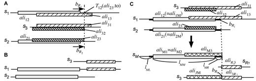
Detail of the domain-splitting procedure. Here, s1 and s2 are the sequences to be merged, and s3 is a sequence similar to either s1 or s2 . The aligned segments on each sequence are indicated by rectangles which have the same pattern for corresponding segments. ( A ) Condition I: the domain boundaries will be extended. ( B ) Condition II: the sequence (in this case, s1 ) will be split. ( C ) Updating the alignment information. In this example, s1 and s2 (upper half) are merged and split into sM and s R 1 (lower half). The thick lines indicate the extended regions. See text for details.
![Post-processing of the clustering algorithm. ( A ) The phylogenetic-tree cutting procedure. The procedure recursively checks whether child clusters of each root node share intra-species paralogs. The three-letter code on each leaf indicates the species name, and the number at each internal node indicates the number of species shared by its child clusters (| Ph ( A ) ∩ Ph ( B )|). ( B ) Rejoining adjacent clusters. Two clusters, A and B , are joined when most of the segments (cutoff ratio radj1 ) belonging to each cluster are adjacent to each other [the segment set adj( A , B )], or almost all of the segments (cutoff ratio radj2 ) belonging to the smaller clusters are adjacent to the other cluster.](https://oup.silverchair-cdn.com/oup/backfile/Content_public/Journal/nar/34/2/10.1093_nar_gkj448/2/m_gkj448f4.jpeg?Expires=1750545297&Signature=FVKIu~A8TsKrZ1NiBl8gdKf-edP0ugndHjgcpE8dudb5N3umq3IuM26n8FZnghILDJGp0N-1mKIR3zjZcrN5FgrajtqKvklia~wrw94vcxq9DnapgDQ1GIvuQC8L3R73AxPj~zHYTYCzZfZ-QGskQeMAXQFRA4QlDn4-Of8n56hLe8bdyko3YJ-7J2VA5IakNQp4dJcg440aJAJE03YIHdXEibhaSq2gL-v7BLQacpcNDj5k-yL85levN9SvpEHVqmOtXZ~KmbywYKwrYNPqja1~zuZbvAa40t7~HU5J48VpheW0YvG4mtyE7MGeEjKvtzqQeADerWLJYOVwp9n~mQ__&Key-Pair-Id=APKAIE5G5CRDK6RD3PGA)
Post-processing of the clustering algorithm. ( A ) The phylogenetic-tree cutting procedure. The procedure recursively checks whether child clusters of each root node share intra-species paralogs. The three-letter code on each leaf indicates the species name, and the number at each internal node indicates the number of species shared by its child clusters (| Ph ( A ) ∩ Ph ( B )|). ( B ) Rejoining adjacent clusters. Two clusters, A and B , are joined when most of the segments (cutoff ratio radj1 ) belonging to each cluster are adjacent to each other [the segment set adj( A , B )], or almost all of the segments (cutoff ratio radj2 ) belonging to the smaller clusters are adjacent to the other cluster.

Orthologous groups of RNA polymerase beta (RpoB) and beta' (RpoC) subunits. ( A ) Hierarchical clustering trees created by the DomClust program. Each domain is drawn in a different color. An abbreviated species name (taken from the COG database; see Supplementary Table S2) is shown on each leaf, which is colored according to the kingdom: salmon, bacteria; khaki, archaea; sky-blue, eukaryotes. ( B ) Schematic illustration of the gene structures of RpoB and RpoC in selected genomes.
CPU time required for clustering the entire dataset
| Methods | COG02 dataset | COG03 dataset | ||||
|---|---|---|---|---|---|---|
| Ta (s) | | H | b | T /| H | (× 10 −6 ) | T (s) | | H | | T /| H | (× 10 −6 ) | |
| DomClust | 65.2 | 3 500 593 | 18.6 | 281.3 | 12 250 884 | 23.0 |
| TribeMCL c | 277.5 | 846210 | 327.9 | 1231.5 | 2833190 | 434.7 |
| Methods | COG02 dataset | COG03 dataset | ||||
|---|---|---|---|---|---|---|
| Ta (s) | | H | b | T /| H | (× 10 −6 ) | T (s) | | H | | T /| H | (× 10 −6 ) | |
| DomClust | 65.2 | 3 500 593 | 18.6 | 281.3 | 12 250 884 | 23.0 |
| TribeMCL c | 277.5 | 846210 | 327.9 | 1231.5 | 2833190 | 434.7 |
a CPU time on a 2.4 GHz Xeon machine.
b The number of pairwise similarities used as input.
c BBH relationships (with the selected parameters, r BH = 0.7 and rcov = 0.4) were used as input.

Comparison of the various clustering methods with the COG recovery test, where evaluation was done according to the numbers of exact, phylo-, 80%- and 60%-MGPs against the 2360 WDOG reference set.
Summary of the selected clusters
| Methods | Selected parameters a | No. of clusters b | |||||
|---|---|---|---|---|---|---|---|
| r BH | rcov | Cutoff c | Total | Split d | Maxsize e | Inparalogs f | |
| SLink | 1.0 | 0.8 | 80 | 2910 | — | 3901 | 1.60 |
| TriLink | 0.8 | 0.4 | 60 | 3134 | — | 1757 | 1.66 |
| TribeMCL | 0.7 | 0.4 | 1.5 | 3652 | — | 1100 | 1.52 |
| gUPGMA | — | — | 60 | 4126 | — | 473 | 1.39 |
| DomClust | — | — | 60 | 4412 | 1302 | 396 | 1.41 |
| COG | — | — | — | 3192 | 971 | 806 | 1.65 |
a The parameter set yielding the best agreement with the COG classification ( MTot ). Note that DomClust uses more parameters. See Supplementary Table S1 for a detailed list.
b The number of clusters comprising genes of at least three phylogenetically distinct organisms.
c Cutoff scores for SLink, TriLink, gUPGMA and DomClust, and the inflation parameter for TribeMCL.
d The number of clusters containing genes that were split into multiple domains.
e The maximum cluster size.
f The average number of inparalogs, which is defined as the sum of cluster sizes divided by the sum of the numbers of organisms included in all clusters. The term ‘inparalog’ is adopted from ref. ( 41 ).
Total number of splitting points and the number of splitting points that agree with COG for each parameter
| Parameters | No. of splitting points (No. of sequences) | |||
|---|---|---|---|---|
| radj1 | radj2 | Total | Agreement with COG a | Within 50 amino acids b |
| 1.0 | 1.0 | 7822 (6665) | 2418 (1978) | 1562 (1474) |
| 0.8 | 0.95 | 5377 (4630) | 2240 (1913) | 1498 (1410) |
| 0.7 | 0.9 | 4374 (3799) | 1998 (1716) | 1337 (1260) |
a The number of sequences split by both DomClust and COG and the number of splitting points on these sequences in DomClust.
b The number of splitting points in DomClust that were located within 50 residues of their corresponding splitting points in COG.

Stability of the clustering methods measured through a comparison of the clusters created from the COG02 and COG03 datasets. Five automatic classification methods and the original COG database (COG) were examined. ( A ) The ratios of the number of clusters created from the COG02 datasets classified into each category. ( B ) The ratios of the number of entries belonging to the clusters classified into each category. Note that ‘domain-merged’ and ‘domain-divided’ are counted only in DomClust and COG.

Orthologous groups containing the E.coli ModE protein, an example of DomClust groups whose domain organizations were changed between the COG02 and COG03 datasets. These clusters were generated using the cutoff score of 80. ( A ) Domain organization of the ModE orthologs generated from the COG02 dataset. ( B ) Domain organization of the ModE orthologs generated from the COG03 dataset. The genes added to the COG03 database but not to the COG02 database are indicated by italic letters. ( C ) Hierarchical clustering tree for Group A and Group B. The root node of each group is encircled. The intraspecies paralogs appearing in both subtrees of the root node of Group B are indicated by bold green text. Here, Hin ( Haemophilus influenzae ) and Pmu ( Pasteurella multocida ) are counted only once, since they are closely related organisms. Consequently, the effective number of overlapping organisms is 2, just half of the total number of organisms in each subtree. This does not satisfy the phylogenetic-tree cutting criterion with the cutoff value of 0.5. ( D ) Hierarchical clustering tree for Group C and Group D. The horizontal bars indicate the points of tree cutting, which generated Group C and Group D. The intraspecies paralogs appearing in both subtrees of the original root node of Group D are indicated by bold green text. In this case, the effective number of overlapping organisms is 4, which exceeds the cutoff of the tree cutting.
The author thanks Drs Naotake Ogasawara and Satoru Kuhara for helpful comments. This work was supported in part by Grant-in-Aids for Scientific Research from MEXT, Japan. Funding to pay the Open Access publication charges for this article was provided by Japan Science and Technology Agency.
Conflict of interest statement . None declared.
REFERENCES
Liu, J. and Rost, B.
Ouzounis, C.A., Coulson, R.M., Enright, A.J., Kunin, V., Pereira-Leal, J.B.
Sonnhammer, E.L., Eddy, S.R., Durbin, R.
Schultz, J., Milpetz, F., Bork, P., Ponting, C.P.
Sasson, O., Vaaknin, A., Fleischer, H., Portugaly, E., Bilu, Y., Linial, N., Linial, M.
Sonnhammer, E.L. and Kahn, D.
Gracy, J. and Argos, P.
Yona, G., Linial, N., Linial, M.
Enright, A.J., Van Dongen, S., Ouzounis, C.A.
Heger, A. and Holm, L.
Enright, A.J. and Ouzounis, C.A.
Goodman, M., Czelusniak, J., Moore, W.M., Romero-Herrera, A.E., Matsuda, G.
Page, R.D.M.
Pellegrini, M., Marcotte, E.M., Thompson, M.J., Eisenberg, D., Yeates, T.O.
Marcotte, E.M., Pellegrini, M., Ng, H.L., Rice, D.W., Yeates, T.O., Eisenberg, D.
Enright, A.J., Iliopoulos, I., Kyrpides, N.C., Ouzounis, C.A.
Overbeek, R., Fonstein, M., D'Souza, M., Pusch, G.D., Maltsev, N.
Eisenberg, D., Marcotte, E.M., Xenarios, I., Yeates, T.O.
Galperin, M.Y. and Koonin, E.V.
Jim, K., Parmar, K., Singh, M., Tavazoie, S.
Tatusov, R.L., Koonin, E.V., Lipman, D.J.
Tatusov, R.L., Natale, D.A., Garkavtsev, I.V., Tatusova, T.A., Shankavaram, U.T., Rao, B.S., Kiryutin, B., Galperin, M.Y., Fedorova, N.D., Koonin, E.V.
Remm, M., Storm, C.E., Sonnhammer, E.L.
Abascal, F. and Valencia, A.
Zmasek, C.M. and Eddy, S.R.
Storm, C.E. and Sonnhammer, E.L.
Cotter, P.J., Caffrey, D.R., Shields, D.C.
Cannon, S.B. and Young, N.D.
Li, L., Stoeckert, C.J., Jr, Roos, D.S.
Storm, C.E. and Sonnhammer, E.L.
Uchiyama, I.
Altschul, S.F., Madden, T.L., Schaffer, A.A., Zhang, J., Zhang, Z., Miller, W., Lipman, D.J.
Smith, T.F. and Waterman, M.S.
Jones, D.T., Taylor, W.R., Thornton, J.M.
Snel, B., Bork, P., Huynen, M.
Tatusov, R.L., Fedorova, N.D., Jackson, J.D., Jacobs, A.R., Kiryutin, B., Koonin, E.V., Krylov, D.M., Mazumder, R., Mekhedov, S.L., Nikolskaya, A.N., et al.
McNicholas, P.M., Mazzotta, M.M., Rech, S.A., Gunsalus, R.P.
Hall, D.R., Gourley, D.G., Leonard, G.A., Duke, E.M., Anderson, L.A., Boxer, D.H., Hunter, W.N.
Sonnhammer, E.L. and Koonin, E.V.
Heger, A. and Holm, L.
Kriventseva, E.V., Fleischmann, W., Zdobnov, E.M., Apweiler, R.

Comments