Statistical implications of the n = 1 observation of 1I/‘Oumuamua Open Access

ABSTRACT

1 INTRODUCTION

Our first interstellar interloper ‘Oumuamua was discovered in October 2017 (Meech et al. 2017; Williams 2017), and much effort has since gone into explaining its formation (Bialy & Loeb 2018; Ćuk 2018; Raymond et al. 2018; Flekkøy, Luu & Toussaint 2019; Luu, Flekkøy & Toussaint 2020; Seligman & Laughlin 2020; Desch & Jackson 2021; Jackson & Desch 2021). Since all these formation models need to be consistent with the existing observation statistics, it becomes important to get a quantitative handle on what this statistical criterion implies.

The statistical problem of extracting the information implied by a single events arose with the 2017 observation of 1I/2017 U1 (‘Oumuamua) (Williams 2017), the first, and so far the only, non-cometary interstellar interloper observed in our Solar system. However, it is also relevant in the context of radio emission from the Milky Way (Jansky 1933), the detection of cosmic X-rays sources (Giacconi et al. (1962)), and gamma-ray bursts (Klebesadel, Strong & Olson 1973). In geophysics, the occurrence of large earthquakes provides another example where small number statistics becomes the key tool to quantify the risk of repeated events (Habermann 1987; Sornette et al. 1996). The question of small number statistics in the context of astrophysics was addressed by Gehrels (1986), who determined close approximations for the confidence limits of the expectation value 〈n〉 given n observations, and also by Kipping (2021).

The conclusions that may be drawn on the basis of a few, or a single observation depend crucially on the type of assumptions that it is natural to make prior to the observation. For instance, the a priori assumption that the observed phenomenon may occur at equally probable rates leads to a different result than the assumption that it may occur at equally probable intervals of time.

The main purpose of this paper is to obtain the exact distribution P_n(λ) for the expected observation rate λ after n ≥ 1 observations are made and the correct a priori assumption is identified, and to obtain the expected recurrence time of objects similar to ‘Oumuamua by means of the Vera C. Rubin Observatory/Large Synoptic Survey Telescope (LSST) programme. The first observation of ‘Oumuamua was made in 2017 by the Pan-STARRS project (Williams 2017), which was initiated in 2008. Many ground-based observations (Bannister et al. 2017; Jewitt et al. 2017; Knight et al. 2017; Meech et al. 2017) followed the first 2017 observation. No other observations that resemble that of ‘Oumuamua, have yet been made, although another interstellar interloper has been observed, the comet 2I/Borisov, which was discovered in 2019 (Guzik et al. 2019). What sets ‘Oumumamua apart in a way that makes it natural to place it in its own class of objects, is in particular its extra-gravitational acceleration (Micheli et al. 2018) that was observed without any detectable outgassing, as well as its light-curve variability (Meech et al. 2017).

The probability of making one or more similar observations some time into the future requires identifying the correct a priori distribution. This brings the problem beyond the simple application of Poisson statistics. Following Kipping (2021), we shall assume that the observations are random and uncorrelated in time, in other words, a Poisson process, and combine this with Bayes theorem. However, in order to minimize the implied bias in the a priori assumption, we apply information theory (Shannon 1948; Shannon & Weaver 1949; Jaynes 1957). The assumption that ‘Oumuamua like objects originate from an unknown number of independent production sites leads to a flat a priori distribution where all rates are equally probable.

In calculating the probability of observing one or more objects similar to ‘Oumuamua based on its detection and a suitable prior distribution, we must include the potential constraints given by estimates of the population densities of non-cometary interstellar objects (ISOs) prior to the detection. Such population densities may be converted to estimates of the future detection probabilities via assumptions on the velocity distribution, the detection volumes of the surveys, the ratio of objects with and without cometary activity and their size distribution (McGlynn & Chapman 1989; Sen & Rana 1993; Moro-Martin, Turner & Loeb 2009; Cook et al. 2016; Engelhardt et al. 2017). However, we will argue that the constraints on λ provided by these early estimates are too far from the actual detection rate to have an impact on the future recurrence probability, as the change of this probability due to the a priori constraints is less than 5  per cent even when the uncertainty in these constraints are ignored.

These considerations are developed quantitatively once we have established the theoretical framework based on Bayes theorem and the Shannon/Jaynes information theory. Finally, we obtain the actual recurrence probability as a function of time and the expected waiting time for the next observation, assuming the enhanced efficiency of the Rubin Observatory survey relative to earlier programmes.

2 DERIVATION OF THE PROBABILITY DISTRIBUTION

We derive the probability density for the observation rate λ given the fact that n observations have been made over a time period τ. This is not the same as the probability that n observations will be made given a known observation rate λ, although the two probabilities are closely linked. The link is provided by the classical Bayes theorem: The probability of having two events A and B, happen may be written

the latter equality constituting the theorem. Here, P(A|B) is the conditional probability of A, knowing that B occurred, and reciprocally for P(B|A), while P(A)(P(B)) is the independent probability that A(B) occurred.

In our context A is the rate λ, and B is the occurrence of the n events. This means that our desired probability P_n(λ) = P(A|B) and P(B) = P(n) is the a priori probability of making exactly n observations during the time τ, given the (lack of) knowledge at the beginning of this period. On the other hand, P(B|A) = P_λ(n) is the probability that n events occur given λ, and P(A) = P(λ) is the a priori distribution of λ. This distribution is the one taken for λ prior to any observations. This leads to the expression

for the distribution we wish to obtain.

2.1 Role of pre-existing constraints on ISO populations

Engelhardt et al. (2017) estimated an upper limit on the interstellar number density of both cometary and non-cometary bodies based on non-detections in Pan-STARRS, the Mt. Lemmon survey, and the Catalina Sky Survey, assuming a cumulative size distribution of such bodies N(D) ∝ D^−2.5 (Dohnanyi 1969). Using this distribution the resulting upper limit found by Engelhardt et al. (2017) on the density ρ of non-cometary bodies larger than 1 km ∼10⁻² au⁻³ translates to an upper limit ρ < 0.5 au⁻³ for the density of bodies larger than 200 m. This the effective spherical diameter of ‘Oumuamua Luu et al. (2020) which has roughly the same cross-sectional area as its assumed oblate or prolate shape.

Moro-Martin et al. (2009) used models for the ejection of protoplanetary material to place an upper limit on the expected detection rate of inactive/small albedo comets by the forthcoming Rubin Observatory. This limit was estimated to a maximum of 1 detection during its 10 yr of planned operation, while Cook et al. (2016) derived an upper limit on the detection of interstellar active comets at 1 detection per year, which is similar to that found later by Hoover, Seligman & Payne (2022).

While Moro-Martin et al. (2009) obtained the ISO density estimates 5 × 10⁻⁹ au⁻³ < ρ < 5 × 10⁻⁵ au⁻³, Sen & Rana (1993) found ρ < 1.6 × 10⁻⁴ au⁻³, and the estimates of Sen & Rana (1993) and McGlynn & Chapman (1989) yield ρ < 10⁻³ au⁻³. Subsequently, Do, Tucker & Tonry (2018) used the ‘Oumuamua detection to estimate the density of non-cometary ISOs to lie around ρ ≈ 0.2 au ⁻³. As a consequence of the ‘Oumuamua observation, Do et al. (2018) suggested the ratio of dry to cometary ISO’s to be around 1000, which is 5–7 orders of magnitude above the ratio that is believed to describe the Oort cloud (Weissman & Levison 1997; Walsh et al. 2011), exo-Oort clouds being assumed to be the sources of ISOs.

It is important to distinguish between a priori assumptions based on model-dependent estimates and a priori knowledge, as only the latter may be used as hard constraints in the P(λ) distribution. Key assumption that went into the λ_min and λ_max estimates prior to the 2017 ‘Oumuamua observation include assumptions on the ratio of dry to cometary ISO’s and the ability of interstellar radiation to convert cometary objects to crusted dry ones. By implication, these assumptions presuppose specific formation scenarios of ejected planetesimals, which only include a few of those proposed for ‘Oumuamua. In particular, they do not include the possibility that ‘Oumuamua is an ultraporous fractal aggregate Luu et al. (2020), a chunk of frozen N₂ ejected from an exo-Pluto like surface (Desch & Jackson 2021; Jackson & Desch 2021), a piece of pure H₂ ice (Seligman & Laughlin 2020), or a solid matrix releasing H₂ upon sublimation (Bergner & Seligman 2023), nor the possibility that it is a light sail developed by an alien civilization (Bialy & Loeb 2018). However, using the estimate of the density of ISOs found by Do et al. (2018), Levine et al. (2021) estimate the expected Rubin Observatory detection rates for ISOs with a range of different formation pathways, albeit with the inclusion of the information that ‘Oumuamua was already detected.

In calculating the probability for another ‘Oumuamua observation based on (1) the a priori information on expected detection rates and (2) the actual detection, it would be inconsistent to include the information of (2) in (1). While the actual detection will lead to estimates of the interstellar density of similar bodies, the detection may not be included in the prior information. As we will show, the pre-existing constraints on detection rates must be within an order of magnitude of the actual detection rate, in order to make a noticeable difference in the probability of making another similar detection. The pre-existing model-based constraints are either too wide, or they have values that are not favoured by probability given the subsequent observation, as is apparent in the adjustments to ratio of cometary to non-cometary bodies that followed the ‘Oumuamua observation (Do et al. 2018).

2.2 Operational efficiency

Following Trilling et al. (2017b), we shall take the effective operational period of Pan-STARRS to have started in 2012, thus accounting for the increase in operational efficiency that had occurred before the 2017 detection of ‘Oumuamua. This yields an effective observation time of τ = 10 yr resulting in n =1 observation.

The Rubin Observatory will survey 20 000 deg² up to a magnitude 24.5 repeatedly over 10 yr. The LSST detection limit is estimated to be three magnitudes deeper than Pan-STARRS’ typical limiting magnitude of ∼21.5, which translates to a factor of three smaller in the size of observable objects (Trilling et al. 2017b). Assuming the small body size distribution N(D) ∝ D^−2.5 it is possible to integrate over the smaller observable sizes as well as the increased number of visible objects. This leads to a yearly observational capacity of the Rubin Observatory survey that is roughly five times that of Pan-STARRS (Trilling et al. 2017a) in terms of the expected number of detections. We denote this performance increase by α. The value of α may be somewhat reduced by the fact that the residence time of ISOs will be larger within the accessible Rubin Observatory observation volume than within that of Pan-STARRS (detecting the same object twice does not lead to an independent detection). This effect is ignored in the following, and we shall simply assume that the enhanced capacity of the Rubin Observatory over earlier observational campaigns may effectively be represented as an increase α ≈5 in the future observational time period τ₁; in other words, that we may include it by the replacement τ₁ → ατ₁, where τ₁ is the future time window.

2.3 The distribution P_λ(n)

The long-time observation rate is λ = N/T where N ≫ n is a large number of observations taken over a long time T ≫ τ. The probability that one of these n events occurs within the time window τ is τ/T, and so the probability to make exactly n observations over a time window τ may be written

when N ≫ n. This result is nothing but the well-known Poisson distribution.

2.4 The a priori distributions

The a priori distributions P(λ) and P(n) of event rates λ and expected number of observations may result from some physical knowledge of the process producing them. Without such prior knowledge our task becomes avoiding to introduce it inadvertently by implication of our choice for P(λ). The idea is to avoid the introduction of arbitrary information.

Here, we shall simply assume that the rate comes from some unknown number N_s of uncorrelated sources so that λ ∝ N_s. In the ‘Oumuamua case such an assumption is natural regardless of the assumed formation theory. In all of these theories, it is a natural a priori assumption that the production sites are independent and their total number unknown. The question of identifying P(λ) then becomes equivalent to finding the distribution Q(N_s) of the source number. In the case where no prior knowledge exists, or is justified, the choice of Q, should thus represent the least possible input of information.

Shannon (Shannon 1948; Shannon & Weaver 1949), and later, Jaynes (Jaynes 1957) formulated an information theory that quantifies the amount of information, or rather uncertainty, that is contained in a certain probability distribution. The uncertainty function that they derived, has the same formal structure as the Gibbs entropy and may be written

where K is a constant. Maximizing this uncertainty function with respect to Q, subject to the constraint of normalizability

leads to the variational problem with respect to Q(N_s)

where γ is a Lagrangian multiplier that may be determined by normalization. The sum over N_s must be constrained by some lower and upper limits. This then gives

or, in other words, Q = constant. This means that the probability P(λ) must be constant as well, and that all a priori event rates are equally probable. This flat distribution corresponds to a minimum input of information. In contrast, some peaked P(λ) distribution would always produce a smaller uncertainty value H, corresponding to the information present in the knowledge of the peak location.

We may normalize the constant a priori distributions to get P(λ) = 1/(N_max − N_min), or more precisely,

where N_max = λ_maxT and N_min = λ_minT are the upper and lower bounds on the expected number of observations during the long time interval T. Above, we have assumed that the total number N of observations may take equally probable values in the range N_min ≤ N ≤ N_max, and, consequently, the increment of λ, Δλ = 1/T.

Note that the a priori probability P(n) does not contain the information of the existing observations. This information is introduced only by setting n = 1 (or some larger value) in the conditional probability P_n(λ). Instead, the a priori probability P(n) is obtained by combining the prior P(λ) and equation (3), which yields

When λ_maxτ ≪ 1 we get P(n = 1) ≈ (λ_maxτ + λ_minτ)/2, which is the relevant limit for most of the pre-existing constraints: Based on estimates of the inactive comet population density Moro-Martin et al. (2009) estimates the Rubin Observatory detection rate at less than 10⁻³ detection per year. Reducing that rate by a factor 5 corresponding to the smaller capacity of Pan-STARRS, gives a value λ_max = 2 × 10⁻⁴ yr⁻¹. Using this a priori constraints sets the probability of making the ‘Oumuamua observation at P(n = 1) ∼ 0.1  per cent. Using instead the value of the population densities arrived at by Sen & Rana (1993) yields P(n = 1) ∼ 0.15  per cent, and that by McGlynn & Chapman (1989) yields P(n = 1) ∼ 1  per cent. These low values strongly suggest that the corresponding constraints on λ are inadequate as hard constraints in our P(λ) distribution. In the following, we will assume that the λ_max and λ_min values are in fact closer to the actual detection rate in order to quantify their role.

Inserting the a priori distributions in equation (2) yields the desired distribution P_n(λ) = p_n(λ)Δλ with the probability density

with n = 1 until the next ‘Oumuamua-like observation is made. This is our desired result for the rate distribution. This function takes its maximum at n/τ, and gives an average 〈λ〉 = (n + 1)/τ, with a standard deviation |$\sqrt{n+1}/\tau$|⁠. Note that the distribution p₁(λ) takes its maximum at λ = 1/τ, which is the historical detection rate, while the expectation value 〈λ〉 = 2/τ. The difference between the actual and expected occurrence rates is due to the skewness of the p(λ)-distribution. This distribution is plotted as a function of λ/λ_max in Fig. 1, assuming that λ_minτ ≪ 1 and λ_maxτ ≫ 1. In the figure, p_n(λ) is multiplied by λ_max, so that the curves remain normalized when integrated over x = λ/λ_max. Note that on this scale, the curves become more peaked when n increases, reflecting a smaller uncertainty in the more probable λ-values relative to the maximum- or average value. However, even with only a single observation n = 1, the spread in λ-values is finite.

Figure 1.

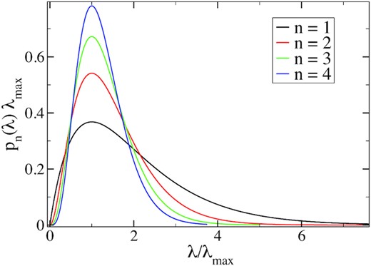
The rate distribution function of equation (10) plotted for different n as a function of the rate normalized by its maximum value.

Open in new tabDownload slide

The assumption made by Kipping (2021) is that P(λ) ∝ 1/λ. Being a power law, this distribution is scale-free, like ours, but produces a different end result. Also, this choice introduces a larger amount of information as quantified by equation (4), than the flat distribution and we therefore select the latter. This choice, which is also known as the Bayes–Laplace uniform prior, was also made by other authors (Cameron 2011) without the justification in terms of information theory. In Cameron (2011), several non-informative priors are assumed; by contrast, the Jaynes uncertainty maximization singles out just one of these.

2.5 Expected waiting times

Now, P_λ(m) of equation (3) is the probability of making exactly m observations within a time τ, given a known value of λ. Replacing τ by a future time interval τ₁ and summing over any number of new observations m ≥ 1 gives the probability of making another observation or more, within the time τ₁ assuming a given λ value,

where we have used the identity |$\sum _{m=0}^\infty x^m/m! = e^x$|⁠. Averaging this probability over all λ-values yields the probability that another observation is made within the future time window τ₁:

where p₁(λ) is given in equation (10) with n = 1. Doing the integration, then gives

where the correction terms due to the assumed constraint values of λ_min and λ_max are

in the limit when λ_minτ ≪ 1 and λ_maxτ ≫ 1. Note from equation (13) that ϵ_min enters as a positive correction while ϵ_max is negative, as an upper bound on λ will reduce detection probabilities, while a lower bound does the opposite. When λ_minτ < 0.1, ϵ_min < 10⁻³, and when λ_maxτ > 10, ϵ_max < 4 × 10⁻⁴, assuming for simplicity that τ = τ₁. This means that in order to affect the predicted detection probability noticeable the a priori constraints on λ must be within a factor 10 of the actual detection rate 1/τ. Otherwise, the actual ‘Oumuamua detection is the only piece of information that determines P_{m ≥ 1}(t), while the estimates of likely detection probabilities based on estimates of the ISO populations by Moro-Martin et al. (2009) only yield a ∼0.1  per cent correction.

The a posteriori ISO density estimate by Do et al. (2018) of ρ ≈ 0.2 au⁻³ was based on the actual λ ≈ 1/τ observation rate. On the other hand, the upper bound of ρ < 0.5 au⁻³ obtained by Engelhardt et al. (2017) was obtained before the ‘Oumuamua observation was made. Since the detection rate is proportional to the population density when all other factors are equal, the factor of 2.5 between the ρ-values, may be taken to yield an estimated a priori upper bound λ_maxτ = 2.5 in this case. This gives ϵ_max = 7 per cent if this λ_max-value is taken as a hard constraint. However, while it is remarkable how close the estimate of Engelhardt et al. (2017) is to the a posteriori estimate it is hardly justified to use it has a hard upper bound, given the scatter in the other prior ρ-estimates and the uncertainty in the underlying model assumptions.

In the following, we well neglect the ϵ_max and ϵ_min terms and replace τ₁ → ατ₁ to account for the increased efficiency of the Rubin Observatory (VRO) survey. Also, the generalization to the case where several observations n exist beforehand, is straightforward. Above, we assumed that only n = 1 observation exists. Given n > 1 observations all that is needed is to replace p₁(λ) by p_n(λ) in equation (12), so that

This integral is easily performed and gives

which is the probability of making one or more observations by the Rubin Observatory during a time window τ_n, provided n observations were already made during the previous time τ, given that Pan-STARRS and other programmes made a single observation during the time τ ≈ 10 yr.

The hypothetical n > 1 case would apply if yet another ‘Oumuamua like observation were made by means of Pan-STARRS. If the question is ‘what is the probability of making a third observation with the Rubin Observatory, given that one observation was made by Pan-STARRS and another by Rubin Observatory’, then the observation time τ would have to be scaled by a factor β > 1 to account for period over which the observation efficiency was increased.

Setting n = 1 again for the actual case, we obtain

for the probability of making another ‘Oumuamua like detection by the Rubin Observatory during a future time window τ₁.

It is interesting to use the above result to evaluate the probability that Pan-STARRS should have made another observation during the 2017–2022 period after the first detection during the 2012–2017 period (in which case n = 1, τ = 5 yr, τ₁ = 4 yr and α = 1). This gives a probability |$P_{\tau _1}(m\ge 1) =$| 69  per cent. By contrast, the assumption made in Kipping (2021) leads to the prediction P_{m ≥ 1}(t) = 1 − τ/(τ₁ + τ) = 44 per cent. In either scenario, the lack of a second detection is quite reasonable.

The confidence level CL is the lower bound on |$P_{\tau _1} (m \ge 1)$|⁠, since this is a cumulative distribution over the time up to τ₁ after n = 1 detection has been made. Equating CL and |$P^{\mathrm{ VRO}}_{\tau _1}(n\ge 1)$| in equation (16) gives the corresponding minimum waiting time

which decreases sharply with increasing n, as expected. In the n = 1 case the minimum waiting time is

This behaviour is illustrated in Fig. 2 where n = 1, the current number of detections. The Rubin Observatory observations should lead to a second ‘Oumuamua-like detection within 5 yr with 90  per cent probability, and one within 1.5 yr with a 66  per cent probability.

Figure 2.

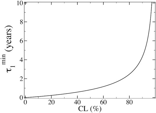
Expected minimum waiting time |$\tau _1^{\mathrm{ min}}$|⁠, to make another observation by means of the Rubin Observatory telescope as a function of the confidence limit CL. This result, which is given in equation (19), is based on the information that the n = 1 observation was already made during the prior time τ = 10 yr.

Open in new tabDownload slide

3 CONCLUSIONS

We have derived the probability distribution for the rate of future ‘Oumuamua-like detections, starting from the knowledge that such an event has indeed occurred. Looking forward to the possibility that more detections are made, we have generalized this result to that case where n > 1 observations exist. The theoretical basis for the rate distribution is a combination of Bayes theorem, Shannons information theory, and the assumption that the events result from a Poisson process. With this distribution in hand, we have also derived the corresponding probabilities for future events to take place as well as the confidence limits of these probabilities. Our main result is the expected recurrence time using the Rubin Observatory program, which is given in terms of the confidence limit in equation (18). Another observation similar to that of ‘Oumuamua is expected within 5 yr at a confidence limit of 90  per cent.

We have applied information theory to minimize the information content implied by the prior distribution, a process that yields a flat a priori distribution over λ values. If, for some reason, knowledge of time correlations is produced, the a priori distribution would need to be changed accordingly. We have quantified the effect of the current prior information relating to the nature of population densities of small interstellar bodies and found that this information must constrain the detection rate λ to within an order of magnitude of the actual detection rate (1 in 10 yr for ‘Oumuamua) to have a noticeable effect on the predicted recurrence probability. Otherwise this prior information will be trumped by the information of the actual detection.

ACKNOWLEDGEMENTS

We thank Knut Jørgen Måløy for valuable discussions and the Research Council of Norway through its Centers of Excellence funding scheme, project number 262644. We are also grateful to Garret Levine for thoughtful remarks and critical comments that greatly improved the discussion in the manuscript.

DATA AVAILABILITY

The data underlying this article, in particular those for Figs 1 and 2, are easily generated from equations (10) and (18). However, they will be shared on request to the corresponding author.

References