


ABSTRACT
The standard model of cosmology describes the matter fluctuations through the matter power spectrum, where |$\sigma _{8} \equiv \sigma _{8,0} \equiv \sigma _{8}(z = 0)$|, defined at the scale of |$8\, h^{-1}$| Mpc, acts as a normalization parameter. Currently, the literature reports measurements of |$\sigma _{8}$| analysing different cosmic tracers, where some of these results were obtained assuming a fiducial cosmology. In this study, we measure, in a model-independent approach, the matter fluctuations in the Local Universe using H i extragalactic sources mapped by the ALFALFA survey. Our analyses allow us to test the standard cosmological model under extreme conditions in the highly non-linear Local Universe, quantifying the amplitude of the matter fluctuations there. Our work directly measures |$\sigma _{8}$| using the three-dimensional distances of the H i sources determined by the ALFALFA survey without assuming a fiducial cosmology, resulting in a robust model-independent measurement of |$\sigma _{8}$|. Our methodology involves the construction of suitable mock catalogues to simulate the large-scale structure features observed in the data, applying the two-point correlation function, and making use of Markov chain Monte Carlo methods to estimate the parameters. Analysing these data, we measure |$\sigma _8 = 0.78 \pm 0.04$| for |$h = 0.6727$|, |$\sigma _8 = 0.80 \pm 0.05$| for |$h = 0.698$|, and |$\sigma _8 = 0.83 \pm 0.05$| for |$h = 0.7304$|. Considering the data pairs |$(\sigma _8, H_0)$| from the Planck cosmic microwave background (CMB) and Atacama Cosmology Telescope (ACT) CMB-lensing analyses, our measurement agrees with them within |$1\, \sigma$| confidence level. From a model-independent perspective, we find that the scale where the matter fluctuation is 1 is |$R = 7.2 \pm 1.5~\text{Mpc}$|.
1 INTRODUCTION
Cosmic structures form by gravitational instability, when matter contained in a sufficiently dense region collapses. The standard cosmological model reproduces quantitatively the main features of the evolution of matter fluctuations through the matter power spectrum. The normalization parameter of this spectrum, |$\sigma _{8} \equiv \sigma _{8,0}$|, is defined as the amplitude of the matter fluctuations at redshift |$z=0$|, at the scale of |$8\, h^{-1}$| Mpc (Peebles 1967; Padmanabhan 1993; Feldman, Kaiser & Peacock 1994; Mo, Van den Bosch & White 2010).
A current tension in the value of |$\sigma _{8}$| is reported in the literature due to the different values obtained using cosmic microwave background (CMB) and large-scale structure (LSS) data (Nunes & Vagnozzi 2021; Virtanen et al. 2020). Notice that the Planck CMB value, |$\sigma _{8}^{\text{Pla}}$|, is not a direct measurement but a derived one, assuming the Lambda cold dark matter (ΛCDM) model to describe the evolution of the primordial perturbations, and using Bayesian analyses to best fit the CMB temperature fluctuations and combining these data with other cosmic probes. As well, the literature reports |$\sigma _{8}$| values obtained through statistical analyses that combine cosmological probes using, sometimes, a model-dependent approach to obtain |$\sigma _{8}$| (Planck Collaboration VI 2020; Heymans et al. 2021; Avila et al. 2022; Madhavacheril et al. 2024).
The cosmological parameter |$\sigma _8$|, which quantifies the matter fluctuation, is related to |$\sigma _8^{\text{tr}}$|, the fluctuation of the cosmic tracer, through a linear bias; |$\sigma _8$| is used to normalize the matter power spectrum, therefore it is a very important parameter in modern cosmology (Kaiser 1988; Juszkiewicz et al. 2010). In general, measurements of |$\sigma _8$| in redshift surveys use cosmic objects that are reliable matter tracers, i.e. |$b \sim 1$|. By measuring the variance of the number density of galaxies, one effectively obtains the variance of matter, enabling a comparison with diverse measurements reported in the literature (Borgani et al. 1995). The fluctuation in the number density of galaxies in the Local Universe is roughly of the order of 1 on scales of |$8\, h^{-1}$| Mpc (h is defined by |$H_0 = 100\, h$| km s|$^{-1}$| Mpc|$^{-1}$|).
Using counts-in-cells (CIC) in the IRAS survey, Efstathiou et al. (1990) found |$\sigma ^2 = 0.26$| at the effective distance |$R = 30\,h^{-1}$| Mpc and |$\sigma ^2 = 0.21$| at |$R = 40\,h^{-1}$| Mpc, in disagreement with the prevailing standard cosmological model of that time, i.e. the CDM with |$\Omega = 1$|, suggesting that the analysed data exhibited more clustering than predicted by the model. In a later study, Efstathiou (1995) revisited this technique with two surveys of IRAS galaxies and found a better agreement with the CDM model. However, taken into account the error interval, other models were also conceivable, such as those with lower values of the matter density parameter, such as the |$\Lambda$|CDM model. Simultaneously, Borgani et al. (1995) conducted an extensive work to validate simulated catalogues in the study of cluster distribution, employing various statistical methods to measure |$\sigma _8$|. The application of this methodology to the Abell/ACO cluster redshift sample showed a preference for the |$\Lambda$|CDM model in explaining Abell/ACO data clustering. More recently, Repp & Szapudi (2020) applying the CIC approach in the SDSS Main Galaxy Sample, constrained b and |$\sigma _8$| simultaneously, obtaining values of |$b = 1.36 \pm 0.14$| and |$\sigma _8 = 0.94 \pm 0.11$|, which agrees well with previous findings. Overall, these studies indicate that at scales close to or above |$8\, h^{-1}$| Mpc, the clustering of galaxies is in excellent agreement with linear perturbation theory, provided that the bias is approximately 1.
The aim of this study is to analyse the mass fluctuations within the Local Universe across several scales, for this, we use as a cosmic tracer the H i extragalactic sources mapped by the ALFALFA survey. One of the main motivations to perform this study is to test the standard cosmological model at extremely low redshift, which means that we are dealing with non-linear scales. In fact, it is well known that the Local Universe exhibits significant non-linear fluctuations in structure growth, providing a unique opportunity to assess the limit of linear theory across various scales (Borgani et al. 1995; Martin et al. 2012; Papastergis et al. 2013; Avila et al. 2018, 2019, 2021; Franco, Avila & Bernui 2024); for this task, we use cosmological distances in real space. Notice that the ALFALFA catalogue provides the distance values of the observed H i sources, where these quantities are not directly measured, instead, they are estimated assuming a semi-analytical velocity field model that uses a default value for |$H_0 = 70$| km s|$^{-1}$| Mpc|$^{-1}$| (Masters 2005). This suggests the possibility that the distances obtained with this flow model could be biased, and our |$\sigma _8$| measurement too. To this end, as explained below, we perform consistency analyses to investigate the impact of assuming this specific value for |$H_0$| in our measurement of |$\sigma _8$| (Jones et al. 2018).
In addition, because the H i sources are effective tracers of dark matter for scales below |$10\, h^{-1}$| Mpc (Martin et al. 2012; Papastergis et al. 2013; Jones et al. 2016), studying the ALFALFA catalogue one can obtain valuable insights into the matter fluctuations in the Local Universe. Observe that |$\sigma _8$| is an important cosmological observable that helps to understand the role of dark matter in the dynamics of cosmic structures growth (Avila et al. 2022). Our analyses differ from others in the literature in that (i) we perform a direct measurement of |$\sigma _{8}$| using the ALFALFA survey data in the Local Universe, |$z \approx 0$|; (ii) we measure |$\sigma _{8}$| for H i extragalactic sources, which are good tracers of matter because |$b \sim 1$| (Obuljen et al. 2019); (iii) we use the three-dimensional distances provided by the ALFALFA catalogue, therefore our analysis is model independent; and (iv) we perform diverse robustness tests to confirm the validity of our results.
Our work is structured as follows: the ALFALFA catalogue is presented in Section 2, which details the process of selecting objects for analyses, as well as the construction of the random catalogues and of the covariance matrix, essential components for our analyses. In Section 3, we elaborate on the methodology used to calculate the matter fluctuations, |$\sigma (R)$|, and its corresponding error. The results of our analyses and our conclusions are presented in Sections 4 and 5, respectively. All robustness tests that support our main results are presented in the appendix.
2 THE ALFALFA CATALOGUE
The ALFALFA survey was initiated in 2005 with the scientific aim of obtaining measurements of the mass and luminosity functions through extragalactic sources in the H i 21 cm line. By its conclusion in 2018, it covered an area in the sky of around |$6900 \deg ^2$| at redshift |$z\,\lt\,0.06$|. At the end, 31 502 H i sources were observed. Due to the limitations of the radio telescope used to detect the H i sources, the observations were divided between the Northern hemisphere (|$7^{\rm h} 20^{\rm m} \lt $| RA |$\lt 3^{\rm h} 15^{\rm m}$|) and the Southern hemisphere (|$7^{\rm h} 20^{\rm m} \lt $| RA |$\lt 21^{\rm h} 30^{\rm m}$|).
The ALFALFA data show a significant distinction based on the signal-to-noise ratio, categorizing them by specific codes: Code 1: involves observations with high signal-to-noise ratio, confirmed in the optical part; Code 2: refers to sources with low signal-to-noise ratio, confirmed in the optical part but considered unreliable; Code 9: relates to high-velocity H i clouds without optical confirmation. In this work, we exclusively use Code 1 sources, following Haynes et al. (2018) (for LSS analyses using the ALFALFA survey, see e.g. Avila et al. 2018, 2021; Franco et al. 2024).
2.1 Data selection
The ALFALFA collaboration estimates distances of the H i extragalactic sources following two approaches, depending if |$cz_{\odot }$| is less than or greater than 6000 km s|$^{-1}$| (Haynes et al. 2018). Because we are interested in studying matter clustering in the Local Universe, we select for analysis the H i sources with |$cz_{\odot } \lt 6000$| km s|$^{-1}$|, corresponding to distances |$\lesssim 85$| Mpc. Moreover, to avoid highly non-linear effects, we consider cosmic objects at distances greater than 20 Mpc. That is, we select for our analysis 3682 H i extragalactic sources of the Local Universe with distances in the range |$20{-}85$| Mpc and with |$cz_{\odot } \lt 6000$| km s|$^{-1}$| (Avila et al. 2021, 2023).
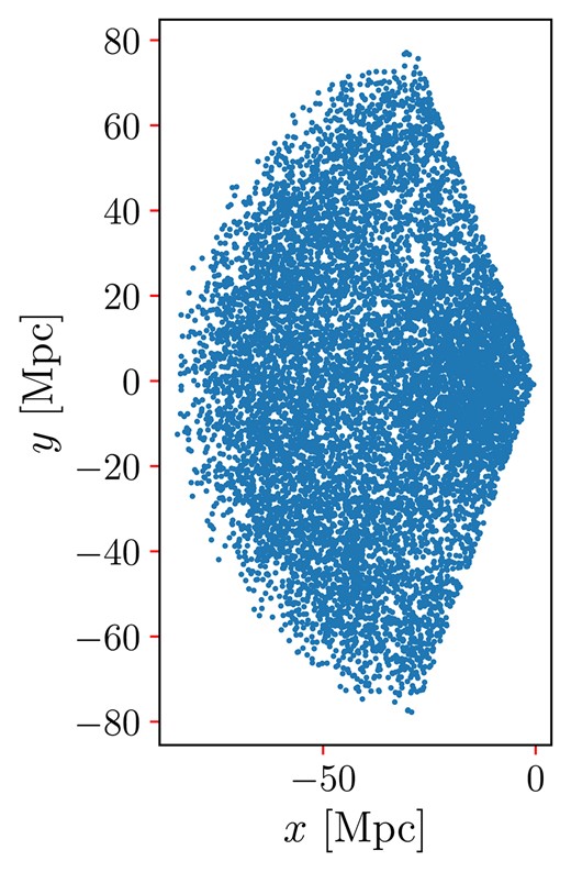
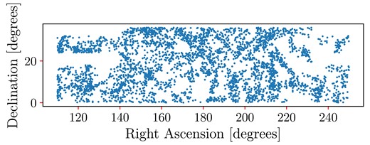
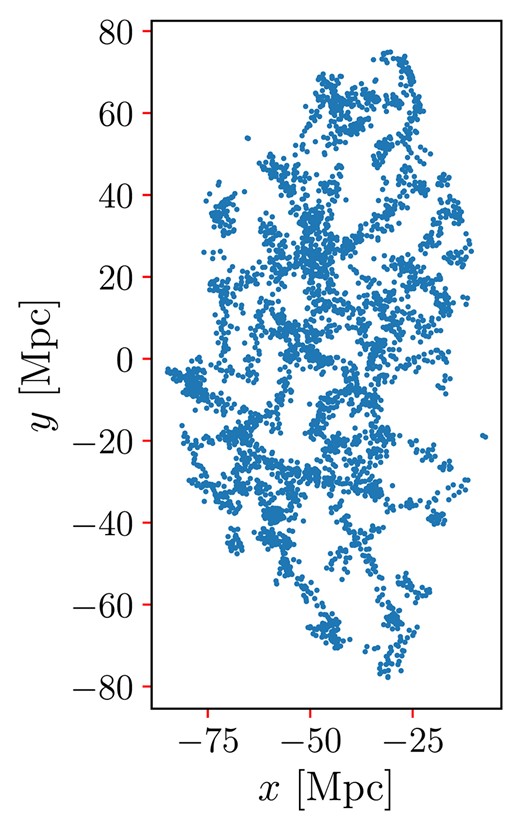
The survey was subdivided into observations conducted in the Northern and Southern hemispheres. In this work, we analyse the region in the Northern hemisphere, which covers a larger area and encompasses a greater number of detected H i sources. Fig. 1 shows the distribution of this sample, while Figs 2 and 3 illustrate the footprint and the Cartesian projection of the selected sample, respectively.
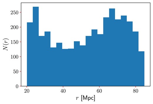
Distances distribution of the selected sample, with 3682 H i extragalactic sources.
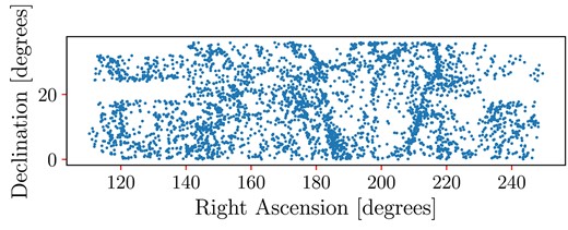
Footprint of the selected sample in equatorial coordinates, localized in the Northern hemisphere.
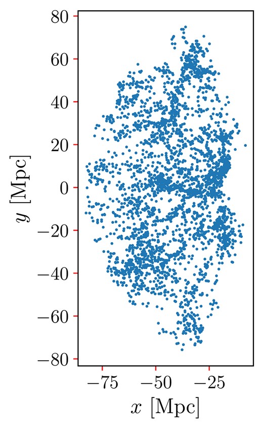
Cartesian projection of the selected sample.
One potential problem in our analyses arises from the fact that distances in the ALFALFA catalogue were not directly measured by the survey but estimated using a semi-analytical flow model that assumes the value |$H_0 = 70$| km s|$^{-1}$| Mpc|$^{-1}$| for the Hubble constant (Masters 2005). To investigate a possible bias of this particular choice of |$H_0$| in our analyses, we produce a number of simulated distance catalogues by randomly sampling the value of the Hubble constant from a Gaussian distribution; then we analyse these simulated data according to our methodology looking for a possible bias in our |$\sigma _8$| measurement. We perform this study in Appendix C.
2.2 Random catalogues
The construction of random catalogues, i.e. a point distribution with the same observational features as the data but without correlations between the objects, is an essential step in obtaining the correlation function, |$\xi (r)$|. The number density of this catalogue is tens of times greater than the sample data in order to reduce the statistical noise in the correlation function (Keihänen et al. 2019; Avila et al. 2024).
For this work, we implemented the publicly available code randomsdss (Chalela 2021)1, which allows us to generate a random redshift distribution from the original measurements while keeping the selection features unchanged. The angular distribution is generated following the algorithm from Franco et al. (2024). The random catalogue has ten times as many points as the data sample. Figs 4 and 5 show the angular coordinates and the Cartesian projection of the random catalogue, respectively.
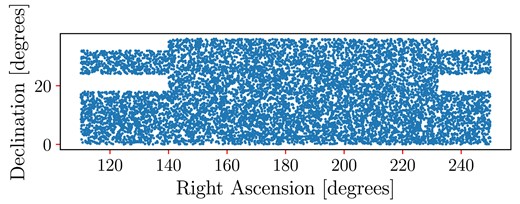
Footprint of the random sample.
Cartesian projection of the random sample with the footprint of the sample in analysis (see Fig. 3).
2.3 Mock catalogues
The LSS of the Universe is better understood knowing the correlation between its components, information that is encoded in the covariance of the two-point correlation function of cosmic objects, like the galaxies. In fact, this function encodes crucial information regarding a galaxy survey, including the survey volume, masking effects, and the average galaxy density (see, for instance, de Santi & Abramo 2022). Calculating the variance of the correlation function needs the evaluation of high-order correlations, however, accurate and accessible methods have been created to estimate it. Martinez & Saar (2001) showed six of such methods, made for specific estimators. These methods usually use either theoretical ideas or the observed galaxy distribution itself to calculate the error, like jackknife and bootstrap techniques (Norberg et al. 2009). Nevertheless, the best method found by Martinez & Saar (2001) uses artificial galaxy distributions, either with N-body simulations or random methods with a known correlation function; it works better because one can obtain the dispersion from multiple correlation function measurements calculated in a way similar to that observed in the sample under analysis.
In this study, we adopt a stochastic model known as Cox processes (Martinez et al. 1998; Pons-Bordería et al. 1999; Gausmann & Ferrari 2024). While this model does not encompass all the non-linear physical processes involved in structure formation, as seen in N-body simulations (Pandey 2010), Cox processes are advantageous due to their simplicity, low computational requirements, and the availability of their analytic two-point correlation function (Martinez & Saar 2001; Avila et al. 2018),
where l and |$L_V$| are parameters of the point process generation. These mock catalogues are constructed in the following way: we distribute |$n_{\rm s}$| segments of length l in a cube of side L. The average number of segments per unit volume, |$\lambda _{\rm s}$|, times the length l defines the density of segments, |$L_{V}=\lambda _{\rm s} l$|. The number of points on each segment is, on average, the same. Let |$\lambda _l$| be the number of points per unit length, then the intensity of the point process is |$\lambda =\lambda _l L_V$|.
Due to the methodology of our analyses, we seek that the correlation function obtained from the Cox processes be close to the correlation function of the H i sources. The dispersion of the n realizations, described above, will represent the error of the correlation function of the sample of H i sources. Thus, the parameters of the Cox process are adjusted in such a way as to reproduce the observational features presented by the sample in analysis. However, an initial step can be taken by assuming the cosmological principle: On sufficiently large scales, the Universe is statistically homogeneous and isotropic. This imposes restrictions on the values of l. It can be shown that the scale of homogeneity in the Cox process is |$R=4\, l$|. Assuming a minimum scale for homogeneity of 100 Mpc, one expects |$l\gt 25$| Mpc. Our procedure starts fixing |$l=25$| and then chose |$L_{V}$| when getting a number density similar to our H i sample.
For this work, we set the following values for the Cox process parameters: |$\lbrace l, L_{V}, \lambda _l\rbrace =\lbrace 25, 0.008, 1.8\rbrace$|. To obtain a representative dispersion, we construct 1000 mocks. In Figs 6 and 7, we show an example of a realization of a Cox process in angular coordinates and its Cartesian projection, respectively. Visually, a realization from the Cox process appears more clustered on small scales. This is because, in order to obtain good agreement on the scales analysed, it was necessary to increase the average number of points on the randomly distributed segments. As we are not analysing a large cosmological volume, we do not observe the correlation function of the H i sources going to zero, and consequently it is difficult to correctly adjust simultaneously all the scales of the Cox process, as l indicates the scale where the equation (1) is zero.
Footprint of a mock realization.
Cartesian projection of a mock realization.
Ultimately, the most important feature needed in these mocks catalogues is that the two-point correlation function of the Cox realizations reproduces at the scales of interest the correlation function obtained with the H i sample data. As a matter of fact, in Fig. 8, we show the difference between the Cox realizations (i.e. the mock catalogues) and the H i sample data. Each curve indicates the difference |$\xi ^{\text{Cox}}_{i}(r)-\xi ^{\mathrm{H\, {\small I}}}(r)$|, where i varies from 1 to 1000. As we can see, there is an excellent agreement for scales above 2 Mpc. This inaccuracy at small scales can be seen in the covariance matrix, calculated as
where N is the sample size, and X and Y represent the correlation values at different bins (i.e. different distances between pairs). In Fig. 9, we show the reduced covariance matrix.
![Upper panel: the two-point correlation functions for the data sample in analysis [$\xi (r)$; red dashed line] and for the 1000 Cox realizations [$\xi _{Cox}(r)$; black solid lines]. Lower panel: difference between the Cox realizations and the data two-point correlation functions, i.e. $\xi _{Cox}(r)-\xi (r)$. Each line corresponds to one realization; we plotted 1000 realizations. We expect the difference to be approximately equal to zero, which occurs on scales above 2 Mpc, due to the difficulties to adjust all scales involved in the Cox process.](https://oup.silverchair-cdn.com/oup/backfile/Content_public/Journal/mnras/537/2/10.1093_mnras_staf088/1/m_staf088fig8.jpeg?Expires=1749157553&Signature=hMT9KHXNqK3AX8YRD-aybnR-Er0nVtjKK-kPI8PnBBqETwUAGCgtMOq-FHkfN~T8~1JH7cNUhDMrBXxbPmEIGw6nQydobGzKFjcQT1gm0wiSy3mMQSqsceAKMYMz-PXt5vNMcm06ZoF0GqAFLjMpK1nL6Jy8Cm4DAgNm56eFZ9MM02eZTomJVPwKY1wja2r2M6C2SGWwOoxSVbqIvDTr3meqbBgMmj~M-dZqx90QRoqN1uj11lj2g~nFMCPE9aXZ96FrvubCDwh7D~WedARbPdAde4d10c9VhN3pC-boD2lUWLUe1BQsiHRDO3rIRC4G5l4lcvw49vEbrnh9ak2LWQ__&Key-Pair-Id=APKAIE5G5CRDK6RD3PGA)
Upper panel: the two-point correlation functions for the data sample in analysis [|$\xi (r)$|; red dashed line] and for the 1000 Cox realizations [|$\xi _{Cox}(r)$|; black solid lines]. Lower panel: difference between the Cox realizations and the data two-point correlation functions, i.e. |$\xi _{Cox}(r)-\xi (r)$|. Each line corresponds to one realization; we plotted 1000 realizations. We expect the difference to be approximately equal to zero, which occurs on scales above 2 Mpc, due to the difficulties to adjust all scales involved in the Cox process.

Reduced covariance (or correlation) matrix, |$\text{Cov}(X, Y)/(\sigma (X)\sigma (Y))$|, obtained from equation (2) and with |$\sigma (X)$| and |$\sigma (Y)$| being the standard deviations of X and Y.
In order to measure the uncertainties for the two-point correlation function obtained using the ALFALFA data, we calculate the two-dimensional covariance matrix |$\text{Cov}(X,Y)$| for the correlation function given in (11). Note that there is a high correlation on small scales, which decreases as we increase the scale. Therefore, by using the covariance matrix in our analyses, we are taking into account for the error evaluation important to quantify systematic effects of the selected sample, such as the sky surveyed area, depth of the survey, numerical density of cosmic objects, etc.
Consequently, the covariance matrix |$\text{Cov}(X,Y)$| provides a more robust measure of the relationships between observational variables, highlighting significant correlations and quantifying the influence of individual variances. In fact, this tool helps to identify possible correlation patterns, and is particularly useful in our study because we are interested in the analyses across different scale distances.
3 THEORETICAL FRAME AND METHODOLOGY
The standard cosmological model describes the mass distribution through the power spectrum of matter density fluctuations, as a function of scale. This function helps to describe the evolution of matter clustering and to understand the problem of structure formation, at several scales. In this section, we explore fundamental concepts to measure the matter fluctuations in the ALFALFA data.
3.1 Matter fluctuations
The physical processes of matter clustering and structure formation began in the early Universe from primordial density fluctuations (Peebles 1967; Padmanabhan 1993; Feldman et al. 1994; Mo et al. 2010). The evolution of these fluctuations is conveniently studied through a dimensionless quantity, the density contrast |$\delta ({\boldsymbol r}, t) \equiv [\rho ({\boldsymbol r}, t)-\rho _{0}(t)]/\rho _0(t)$|. Consider the matter density contrast at a given time in the early Universe, |$\delta ({\boldsymbol r}) = \delta ({\boldsymbol r}, t_i)$|, assume that at different spatial locations |$\delta ({\boldsymbol r})$| is very weakly correlated, i.e. it is a random variable (Padmanabhan 1993). From this, one finds that its Fourier transform, |$\delta _{\mathbf {\it k}}$|, is Gaussian, therefore |$\delta _{\mathbf {\it k}}$| is completely specified by its two moments: zero mean |$\langle \delta _{\mathbf {\it k}} \rangle = 0$| and variance |$\sigma _k^2 \equiv \langle |\delta _{\mathbf {\it k}}|^2 \rangle$|, where |$\sigma _k^2$| is the power spectrum of the density fluctuations, commonly termed |$P(k)$|. The power spectrum, |$P(k)$|, is the Fourier transform of the two-point correlation function, |$\xi (r)$|, which is a primary estimator of the large-scale matter distribution
A way to describe the clustering strength of a given ensemble of cosmic objects is to calculate the variance of the number counts within randomly placed spheres of a given radius R, which, considering the linear perturbations, can be written as
where |$W_{R}$| is the top-hat window with spherical symmetry (Mo et al. 2010). The variance of galaxy, or cosmic objects, distribution is used to normalize |$P(k)$| in equation (3). The function |$\sigma ^2(R)$| can be understood in terms of the variation in mass in a set of randomly placed windows, then one can show that the mass variance is (Mo et al. 2010)
where |$\Delta M \equiv M({\bf \it x},R)-M_0(R)$|, |$M({\bf \it x},R)$| is the mass in a window centred at |${\bf \it x}$|, and |$M_0(R)$| is the average of the mass defined at the scale R. It is also possible to write |$\sigma ^{2}(R)$| as
where |$\Delta _{k}^2$| is a dimensionless quantity proportional to the power spectrum and which expresses the contribution to the variance by the power in a unit logarithmic interval of k (Padmanabhan 1993),
It is useful to define the following quantity, which is related to |$\xi (r)$| by (Padmanabhan 1993)
where this function gives us information about the spatial distribution of objects, because it represents weighted average of correlation function across different scales. Another way to represent |$J_3(R)$| is
where we note that combining equations (6) and (9) we obtain
therefore, knowing |$J_3(R)$| it is possible to calculate the mass variance at the scale R, i.e. |$\sigma ^{2}(R)$|. Finally, one defines |$\sigma _8 \equiv \sigma (R=8\, h^{-1}\, \text{Mpc})$|, at the scale |$R = 8\, h^{-1}$| Mpc.
3.2 Correlation function
We have previously seen in Section 3.1 that it is possible to relate the two-point correlation function with the matter variance on different scales through equations (8) and (10). Therefore, we shall apply the two-point correlation function |$\xi (r)$| to the ALFALFA catalogue to calculate the matter variance. The most widely used correlation function estimator is the Landy–Szalay (Landy & Szalay 1993), that returns the smallest discrepancies for a given cumulative probability, has no bias and nearly Poisson variance (Kerscher, Szapudi & Szalay 2000). This estimator is given by
where |$DD(r)$| is the number of pairs in the sample data with distance separation r, normalized by the total number of pairs; |$RR(r)$| is a similar quantity, but for the pairs in a random sample; and |$DR(r)$| corresponds to a cross-correlation between a data object and a random object. Using |$\xi (r)$| it is possible to determine the excess probability of finding two points from a data set at a given distance separation r when compared to a random distribution. In practice, to obtain |$\xi (r)$| we use the treecorr code (Jarvis, Bernstein & Jain 2004).2
3.2.1 Power-law approximation
The expectation regarding the two-point correlation function is that it behaves according to a power law (Peebles 1993; Papastergis et al. 2013), that is,
where |$r_0$| is a scale parameter that determines the characteristic scale of the correlation, and the parameter |$\gamma$| quantifies the clustering of the cosmic tracer in study.
3.2.2 Constraining power-law parameters using Bayesian inference
In order to determine the optimal power-law parameters, |$r_0$| and |$\gamma$|, from the correlation function measurements, we adopt a Bayesian analysis approach (for more details, see e.g. Verde 2010; Hobson et al. 2014; Trotta 2017). This involves exploring the parameter space using the Markov chain Monte Carlo (MCMC) algorithm implemented through the publicly available emcee3 code (Goodman & Weare 2010; Foreman-Mackey et al. 2013).
In Bayesian analysis, our aim is to determine the probability of a given model with parameters |$\boldsymbol {\theta }$| given a set of observations |$\boldsymbol {D}$|. This involves computing the posterior probability distribution |$P(\boldsymbol {\theta }|\boldsymbol {D})$|, which is given by
where |$P(\boldsymbol {D}|\boldsymbol {\theta })$| is the likelihood function, |$P(\boldsymbol {\theta })$| is the prior distribution, and |$P(\boldsymbol {D})$| is the evidence. As |$P(\boldsymbol {D})$| can be treated like a normalization, we can look only for the scaled posterior. The logarithm of the scaled posterior distribution can be expressed as
where the likelihood can be written as
In this work,
where |$\xi (r_i)$| represents the measured correlation function, |$\xi ^{\text{PL}}(r_i;r_0,\gamma)$| is the model prediction with power-law parameters |$r_0$| and |$\gamma$|, and |$C_{i,j}^{-1}(r_i,r_j)$| is the inverse covariance matrix of the measurements, given by equation (2).
In retrospect, looking at the work of Martin et al. (2012), we have properly selected the space parameter prior, as indicated in Table 1.
Prior ranges and initial guesses for the power-law parameters.
| Parameter | Range | Initial guess |
|---|---|---|
| |$r_0$| | |$1 ~\text{Mpc} ~\lt~ r_0 \lt ~ 15 ~\text{Mpc}$| | 5.0 Mpc |
| |$\gamma$| | |$1 \lt \gamma \lt 3$| | 1.8 |
| Parameter | Range | Initial guess |
|---|---|---|
| |$r_0$| | |$1 ~\text{Mpc} ~\lt~ r_0 \lt ~ 15 ~\text{Mpc}$| | 5.0 Mpc |
| |$\gamma$| | |$1 \lt \gamma \lt 3$| | 1.8 |
4 RESULTS AND DISCUSSION
Applying the statistical tools outlined in Section 3, we analysed the selected sample described in Section 2. First, we calculated the two-point correlation function, |$\xi (r)$|, for our data sample for pair distances in the interval |$[0.5, 15]\, \text{Mpc}$|; our result can be seen in Fig. 10, where we consider 20 bins. Similarly, we applied the same procedure to a set of 1000 mock catalogues generated from the Cox process, as detailed in Section 2.3, to estimate the covariance matrix using equation (2) and subsequently determine the uncertainties associated with our results. The findings are illustrated in Fig. 10.
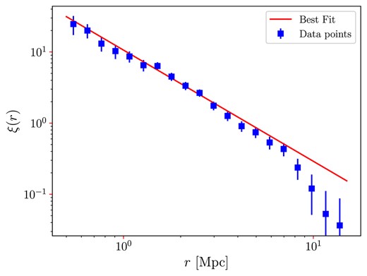
Two-point correlation function for the H i sample in study using, 1000 realizations of the Cox process to estimate the uncertainties. For the best fit, it was assumed the power-law relationship (equation 12).
The best-fitting curve was plotted considering the power law shown in equation (12), performed over the interval |$[0.5, 15]\, \text{Mpc}$|, where the fitting parameters |$r_{0} = 4.5 \pm 0.3\, \text{Mpc}$| and |$\gamma = 1.55 \pm 0.07$| were obtained using the MCMC method (cf. Section 3.2.2 and Fig. 11). The data agree well with the expected power-law function up to |$r \simeq 7\, \text{Mpc}$|. Beyond this scale, the observed decline in the data with respect to the best fit, is indicative of a limited sample volume, and the power-law correlation function does not suitably describe the distribution of matter structures (Martin et al. 2012).
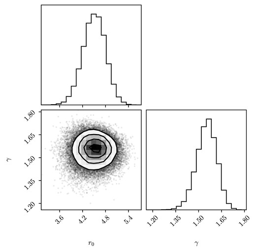
Joint and marginal distributions of the power-law parameters |$r_{0}$| and |$\gamma$|.
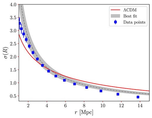
To deepen our analysis, we calculated the |$\sigma (R)$| values. By using the |$\xi (r)$| values and the previously obtained covariance matrix, we can get the mass fluctuation function, which is shown in Fig. 12. The data points were obtained directly from the square root of equation (10) leading to a direct measurement of the matter fluctuation of the H i extragalactic sources, |$\sigma _{8}^{\text{tr}} = \sigma _{8}^{\mathrm{H\, {\small I}}} = 0.92 \pm 0.05$| at scales |$r=8$| Mpc. The red continuous line in Fig. 12 was generated using the Core Cosmology Library4 (CCL; Chisari et al. 2019), which offers a robust computational tool for our calculations. This line corresponds to the theoretical prediction for matter fluctuations modelled under the assumption of Planck’s flat-|$\Lambda$|CDM model (Planck Collaboration VI 2020), with the cosmological parameters specified in Table 2.
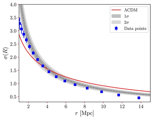
Mass fluctuation for the selected H i sample from ALFALFA. The best fit was assumed to follow a power law, equation (12). The shaded grey areas correspond to |$1\sigma$| and |$2\sigma$| confidence levels. Note that there is an intersection between the data best-fit and the theoretical model |$\Lambda$|CDM, suggestive of a transition between non-linear and linear scales in the behaviour of |$\sigma (R)$|. Beyond this scale, the matter fluctuation of the H i sample consistently falls below the |$\Lambda$|CDM prediction, implying an antibias in our sample relative to the underlying matter.
| Parameter | Value |
|---|---|
| |$\Omega _{\rm c}$| | 0.2656 |
| |$\Omega _{\rm b}$| | 0.0494 |
| h | 0.6727 |
| |$n_{\rm s}$| | 0.9649 |
| |$\sigma _8$| | 0.8120 |
| Parameter | Value |
|---|---|
| |$\Omega _{\rm c}$| | 0.2656 |
| |$\Omega _{\rm b}$| | 0.0494 |
| h | 0.6727 |
| |$n_{\rm s}$| | 0.9649 |
| |$\sigma _8$| | 0.8120 |
| Parameter | Value |
|---|---|
| |$\Omega _{\rm c}$| | 0.2656 |
| |$\Omega _{\rm b}$| | 0.0494 |
| h | 0.6727 |
| |$n_{\rm s}$| | 0.9649 |
| |$\sigma _8$| | 0.8120 |
| Parameter | Value |
|---|---|
| |$\Omega _{\rm c}$| | 0.2656 |
| |$\Omega _{\rm b}$| | 0.0494 |
| h | 0.6727 |
| |$n_{\rm s}$| | 0.9649 |
| |$\sigma _8$| | 0.8120 |
The dashed grey line is the best-fitting expectation for the function |$\sigma (R)$| when one assumes the power law for the two-point correlation function, because of this we call this dashed grey line as the |$\sigma$|-model. We observe a good agreement, at |$2\sigma$| level, between the |$\sigma$|-model and the data. As noticed above the two-point correlation function does not follow a power law for scales above 7 Mpc, in consequence, this fact is translated to the |$\sigma (R)$| computation, and manifests increasing the discrepancy between |$\sigma$|-model and data, as observed in Fig. 12. For both the |$\sigma$|-model and the data, there is a transition with respect to the |$\Lambda$|CDM model around 4 Mpc, suggestive of a possible transition between non-linear to linear scales. As the scale increases, both |$\sigma$|-model and data fall below the |$\Lambda$|CDM model, consistently, indicating that the H i sources are antibiased with respect to the underlying matter fluctuation field (Basilakos et al. 2007).
The scale where our best-fitting data intersects the |$\Lambda$|CDM model, which results from a linear theory, is suggestive of the transition between the non-linear and linear regimes. We find, however, that a more appropriate scale would be to consider the scale where the matter fluctuation is |$\sigma (R) = 1$|, because such scale would be a model-independent quantity in data analyses where distances scales are in Mpc units (and not |$h^{-1}$| Mpc). When we apply this condition to our best-fitting analysis (see Fig. 12) we obtain |$R = 7.2 \pm 1.5~\text{Mpc}$|. This could be considered as the transition scale where the linear relationship is valid |$\delta _{\mathrm{H\, {\small I}}}=b_{\mathrm{H\, {\small I}}}\delta _{M}$|, i.e. the fluctuation of matter of the H i sources is proportional to the fluctuation of underlying matter.
To determine |$\sigma _8$| from our measurement, |$\sigma _{8}^{\mathrm{H\, {\small I}}}$|, it is essential to assume a value for the linear bias, |$b_{\mathrm{H\, {\small I}}}$|. This linear bias, in turn, requires assuming a normalization, |$\sigma _8$|, for the power spectrum when performing statistical analyses that compares models and observations (Basilakos et al. 2007). In summary, our |$\sigma _8$| measurement serves as a consistency test for the |$\Lambda$|CDM model. However, within our approach we can study the effect of the Hubble constant on our |$\sigma _8$| measurement, since one must assume a value of h in order to transform the Mpc units to |$h^{-1}~\text{Mpc}$| units.
Considering the linear bias for the H i extragalactic sources obtained by Obuljen et al. (2019), |$b_{\mathrm{H\, {\small I}}} = 0.875 \pm 0.022$|, and using the relation
with uncertainties given by
we conclude that |$\sigma _{8} = 1.05 \pm 0.06$| at the scale of 8 Mpc. Furthermore, we consider a set of values for the Hubble parameter: |$h = \lbrace 0.6727,\, 0.698,\, 0.7304\rbrace$| to determine the |$\sigma (R)$| at the scale |$R = 8\,h^{-1}\, \text{Mpc}$| in each case. The results, with their respective uncertainties, taking into account the bias are listed in Table 3.
Our measurements of |$\sigma _{8}^{\mathrm{H\, {\small I}}}$| and |$\sigma _{8}$| at the scale |$8\, h^{-1}\, \text{Mpc}$| considering diverse measurements of h.
Our measurements of |$\sigma _{8}^{\mathrm{H\, {\small I}}}$| and |$\sigma _{8}$| at the scale |$8\, h^{-1}\, \text{Mpc}$| considering diverse measurements of h.
As can be seen in the plots of the probability density functions shown in Fig. 13 and in the |$H_{0}{-}\sigma _{8}$| parameter space in Fig. 14, considering the tension metric between two estimates A and B,
we find that our measurements of |$\sigma _8$| agrees at |$0.79\, \sigma$| and |$0.36\, \sigma$| confidence levels with Planck (Planck Collaboration VI 2020) and Atacama Cosmology Telescope (ACT; Madhavacheril et al. 2024) results, respectively.
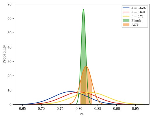
Probability distribution function of |$\sigma _{8}$| for different values of the Hubble parameter h.
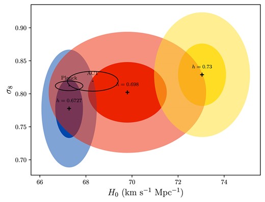
|$H_{0}{-}\sigma _{8}$| parameter space for different values of h. The probability ellipses show |$1\sigma$| and |$2\sigma$| CL. We compare our results with the ACT and Planck data.
Despite |$\Lambda \text{CDM}$| model best fits observational data, it still faces significant challenges, such as the tensions arising from measurements of the Hubble constant, |$H_{0}$| and |$\sigma _{8}$|. Within the |$\Lambda \text{CDM}$| framework, measurements using CMB data yield |$H_{0} = 67.27 \pm 0.60$| km s|$^{-1}$| Mpc|$^{-1}$| (Planck Collaboration VI 2020), whereas local measurements using Type Ia supernovae obtain |$H_{0} = 73.04 \pm 1.04$| km s|$^{-1}$| Mpc|$^{-1}$| (Riess et al. 2022), indicating a discrepancy of |$\sim 5\sigma$| between direct and indirect measurements (Di Valentino et al. 2021a, c; Perivolaropoulos & Skara 2022; Tully et al. 2023; Verde, Schöneberg & Gil-Marín 2024). Regarding |$\sigma _{8}$|, Planck Collaboration VI (2020) report a value of |$\sigma _{8} = 0.8120 \pm 0.0073$|, which is corroborated by Madhavacheril et al. (2024), where |$\sigma _{8} = 0.819 \pm 0.015$|, but they both disagree with direct measurements, such as weak lensing, redshift-space distortions (RSD), and galaxy clustering at |$3\sigma$| level (Di Valentino et al. 2021b; Adhikari et al. 2022; Perivolaropoulos & Skara 2022).
The search for alleviating these tensions motivated numerous recent studies, which report values of |$\sigma _{8} \sim 0.75$| (Tröster et al. 2020; Freedman 2021; Heymans et al. 2021; Nunes & Vagnozzi 2021; Qu et al. 2024). As illustrated in Fig. 14, each value of h provides a distinct value of |$\sigma _{8}$| in units of |$h^{-1}$| Mpc. Our |$\sigma _{8}$| measurement obtained through the ALFALFA data agrees at |$0.79\, \sigma$| with the value reported in Planck Collaboration VI (2020), using for this comparison the h value provided by the Planck Collaboration. Similarly, when adopting the value calculated by Freedman (2021), |$h = 0.698$|, we remain |$0.36\, \sigma$| away from the value reported by Madhavacheril et al. (2024). Some authors suggest that, despite the |$\sigma _{8}$| tension potentially arising from systematic errors (in either CMB or LSS evaluation) or sample variance (originated from different regions observed by different surveys), it may indicate the necessity for a new physics beyond the standard model to explain the tension in |$\sigma _{8}$| and |$H_{0}$| (Nunes & Vagnozzi 2021; Virtanen et al. 2020; Adhikari et al. 2022; Amon & Efstathiou 2022; Perivolaropoulos & Skara 2022; Schöneberg et al. 2022; Poulin et al. 2023; Adil et al. 2024; Akarsu et al. 2024; Chen et al. 2024; Hollinger & Hudson 2024). Nevertheless, we can safely conclude that, considering the data pairs |$(\sigma _8, H_0)$| from the Planck CMB and ACT CMB-lensing analyses, our |$\sigma _8$| measurement agrees with them in less than |$1\sigma$| confidence level.
5 CONCLUSIONS
The search for the cosmological model that describes the observed Universe on large scales motivate the use of astronomical data to explore alternative models through diverse approaches (Marques et al. 2019; de Carvalho et al. 2020; Krishnan et al. 2022; Luongo et al. 2022; Dinda 2024; Dinda & Banerjee 2024; Giarè 2024; Giarè et al. 2024; Oliveira et al. 2024; Ribeiro, Bernui & Campista 2024). In this scenario, the measurement of the galaxies density fluctuation in the Universe is a crucial feature for understanding its LSS, making the determination of the |$\sigma _8$| parameter an important task in modern cosmology. It is estimated that this fluctuation in the Local Universe is approximately 1 on scales of |$8 \, h^{-1}$| Mpc (Juszkiewicz et al. 2010). Over the years, various research teams have come together to measure the matter fluctuations using diverse techniques and cosmic tracers (Hamana et al. 2003; Melchiorri et al. 2003; Reid et al. 2010; Hasselfield et al. 2013), seeking a better understanding of the tendency for galaxies to cluster more densely than the underlying dark matter and the amplitude of primordial fluctuations in the Universe, resulting from physical processes during its early stages. The amplitude of mass fluctuations describes the normalization of the linear spectrum of mass fluctuations in the early Universe, as described in Section 3.1, the spectrum that seeded galaxy formation. Thus, massive clusters form from outlier fluctuations of the primordial Gaussian density field, this means that their abundance is exponentially sensitive to the overall normalization (Bahcall & Bode 2003).
The increasing tension surrounding the value of |$\sigma _8$| necessitates additional studies and analyses with varied data sets and different methodologies to obtain a more precise and comprehensive understanding of matter fluctuation amplitudes in the Universe. In our work, we analysed the LSS of the Universe using data from the ALFALFA extragalactic H i survey. Our focus was on characterizing matter fluctuations and understanding mass variance on different spatial scales, utilizing the H i extragalactic sources as tracers of the underlying matter distribution.
We investigated the matter fluctuation |$\sigma (R)$| by applying the two-point correlation function to a selected sample of the ALFALFA survey, and using the relation between this quantity and |$J_{3}(R)$|. The derived value of |$\sigma _{8}^{\mathrm{H\, {\small I}}} = 0.92 \pm 0.05$| aligns with the expectations for galaxy distribution and is consistent with the prediction of the |$\Lambda \text{CDM}$| model for a sample with bias factor |$b \lt 1$|. When we consider the bias for H i sources, |$b_{\mathrm{H\, {\small I}}}$|, this yields |$\sigma _{8} = 1.05 \pm 0.06$|. Considering different values for the Hubble parameter, we found that each value of h provides a distinct value of |$\sigma _{8}$|, which is different from the previous measurements from Planck and ACT at |$0.79\sigma$| and |$0.36\sigma$|, respectively.
Our results obtained from the analyses of the ALFALFA data highlight the robustness of our methodology to measure the matter fluctuations in the Local Universe, potentially contributing to the ongoing discussion concerning the |$\sigma _{8}$|, or |$S_8$|, tension.
ACKNOWLEDGEMENTS
CF and ML thank Coordenação de Aperfeiçoamento de Pessoal de Nível Superior (CAPES), JO and AB acknowledge to Conselho Nacional de Desenvolvimento Científico e Tecnológico (CNPq), for their corresponding fellowships. FA thanks CNPq and Fundação Carlos Chagas Filho de Amparo à Pesquisa do Estado do Rio de Janeiro (FAPERJ), Processo SEI 260003/014913/2023, for the financial support.
DATA AVAILABILITY
The data underlying this article will be shared on reasonable request to the corresponding author.
Footnotes
REFERENCES
APPENDIX A: ROBUSTNESS TEST WITH CURVE FITTING
For robustness, in this appendix, we also conducted a curve fitting of the data for the theoretical function (12), using the scipy.optimize5 (Virtanen et al.2020) package from the open source library in python language, where we performed the best-fitting analysis of the parameters |$\gamma$| and |$r_{0}$|, in order that they minimize the |$\chi ^{2}$| function defined in equation (16), where Cov|$^{-1}$| is the inverse of the covariance matrix, and Cov is specified in equation (2). The uncertainties of the adjusted parameters, |$\lbrace \sigma _i \rbrace$|, are given by the square roots of the diagonal elements of the covariance matrix, |$\sigma _i = \sqrt{\text{Cov}_{ii}}$|.
In Fig. A1, the fit is shown the best-fitting curve, where we obtain |$r_0 = 4.5 \pm 0.4 \text{; and} \, \gamma = 1.56 \pm 0.11$|. As observed in Table A1, the adjusted parameters values are the same as those obtained using the MCMC method, with an increase in measured error bars, which is expected due to the difference in the methods employed.
Mass fluctuation analysis for the H i selected sample, this time using the curve-fitting method.
The adjusted parameters using MCMC- and curve-fitting methods.
| |$r_0$| (Mpc) | |$\gamma$| | |
|---|---|---|
| MCMC | |$4.5 \pm 0.3$| | |$1.55 \pm 0.07$| |
| Curve fitting | |$4.5 \pm 0.4$| | |$1.56 \pm 0.11$| |
| |$r_0$| (Mpc) | |$\gamma$| | |
|---|---|---|
| MCMC | |$4.5 \pm 0.3$| | |$1.55 \pm 0.07$| |
| Curve fitting | |$4.5 \pm 0.4$| | |$1.56 \pm 0.11$| |
APPENDIX B: THE IMPACT OF THE VIRGO CLUSTER AS A NON-LINEAR EFFECT
Our |$\sigma _8$| measurement was obtained for an ensemble of cosmic objects with distances in the interval |$20{-}85$| Mpc, a purposeful choice to avoid the overdense spatial region, where |$\delta \gt 1$|, containing the Virgo cluster. In this appendix, we study the impact of the presence of the Virgo cluster in our measurement. For this, we analyse the H i objects with distances in the interval |$10{-}85$| Mpc, which includes the Virgo cluster. At the same time, considering for this test those cosmic objects that are closer to us we are also increasing a systematic effect sourced by large peculiar velocities (Migkas et al. 2021; Avila et al. 2023; Kalbouneh, Marinoni & Bel 2023; Lopes et al. 2024).
We perform this consistency analysis recalculating the |$\sigma (R)$| function. Our result is shown in Fig. B1, where for comparison we also plot the original case. As expected, some differences can be observed, being the difference more noticeable at the smaller scales where the clustering, that is, the value of |$\sigma (R)$|, is bigger, presumably due to the presence of more clustered structures like Virgo.
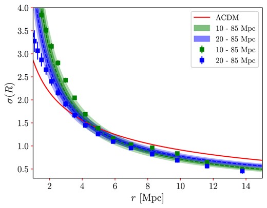
Comparison between two ALFALFA samples with H i sources belonging to distinct distance intervals. The green points correspond to the sample with sources in the interval |$10{-}85~\text{Mpc}$|; the blue points corresponds to sources in the interval |$20{-}85~\text{Mpc}$|. The shaded areas correspond to |$1\sigma$| and |$2\sigma$| confidence levels for each sample.
Nevertheless, in both cases |$\sigma (R)$| agrees at the |$2 \sigma$| level, confirming the robustness of our measurement.
APPENDIX C: CONSISTENCY TEST: IS THE ALFALFA DISTANCE DATA BIASED WITH |$H_0=70$| km s|$^{-1}$| Mpc|$^{-1}$|?
The ALFALFA collaboration provides the distance values of the H i sources, but these quantities were not directly measured but estimated assuming a semi-analytical velocity field model that uses |$H_0 = 70$| km s|$^{-1}$| Mpc|$^{-1}$| for the Hubble constant (Masters 2005). Clearly, this hypothesis opens up the possibility that the distances released in the ALFALFA catalogue could be biased, and our |$\sigma _8$| measurement too. To assess the potential influence of this specific |$H_0$| value on our analysis, we performed a Monte Carlo (MC) procedure to generate a set of simulated catalogues of distances, termed pseudo data, with different values of |$H_0$| randomly chosen from a Gaussian distribution.
To produce 100 MC realizations with simulated distance data sets we proceed as follows. For the kth MC realization, for |$k=1, \cdots , 100$|, the corresponding radial distance of the ith cosmic object, |$\rm{\bf R}^{i}$|, is obtained from
where |$H_0 = 70$| km s|$^{-1}$| Mpc|$^{-1}$|, |$r^{i}$| is the radial distance listed in the ALFALFA catalogue for the ith cosmic object, and |$H_{0}^{k}$| is a value randomly selected from a Gaussian distribution with mean |$\overline{H_0} = 70$| km s|$^{-1}$| Mpc|$^{-1}$| and standard deviation |$\sigma _{H_0} = 1$| km s|$^{-1}$| Mpc|$^{-1}$|.
The kth realization provides the distance set |$\lbrace \rm{\bf R}^{i} \rbrace _k$|. Each one of these pseudo data sets, |$\lbrace \rm{\bf R}^{i} \rbrace _k$|, is analysed according to our methodology as it were the original data to calculate the function |$\sigma (R)^k$| for |$k = 1,\cdots , 100$|. Finally, the set of these functions, |$\lbrace \sigma (R)^k \rbrace$|, is then plotted in Fig. C1, and compared with our original result shown in Fig. 12. As shown by this analysis, our measurement of |$\sigma _8$| is not biased with the specific value of |$H_0=70$| km s|$^{-1}$| Mpc|$^{-1}$|.
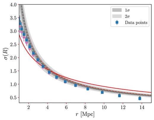
Mass fluctuation analysis for the selected data sample from ALFALFA (blue squares), together with the analysis of the MC realizations of different distance data sets |$\lbrace \rm{\bf R}^{i} \rbrace _k$|, |$k=1,\cdots ,100$| (coloured dots). The blue squares with error bars and the shaded grey areas, corresponding to |$1\sigma$| and |$2\sigma$| confidence levels, are the same as in Fig. 12. For |$r \gtrsim 6$| Mpc, the squares hide the dots.
