


ABSTRACT
Weak gravitational lensing simulations serve as indispensable tools for obtaining precise cosmological constraints. In particular, it is crucial to address the systematic uncertainties in theoretical predictions, given the rapid increase in galaxy numbers and the reduction in observational noise. Both on-the-fly and post-processing methods for constructing lensing light-cones encounter limitations due to the finite simulated volume, necessitating the replication of the simulation box to encompass the volume to high redshifts. To address this issue, our primary focus lies on investigating and quantifying the impact of box replication on the convergence power spectrum and higher order moments of lensing fields. Subsequently, a univariate model is utilized to estimate the amplitude parameter A by fitting four statistics measured from partial sky light-cones along specific angles, to the averaged result from random directions. The investigation demonstrates that the systematic bias stemming from the box replication phenomenon falls within the bounds of statistical errors for the majority of cases. However, caution should be exercised when considering high-order statistics on a small sky coverage (|${\lesssim} 25~\mathrm{deg^2}$|). For this case, we have developed a code that facilitates the identification of optimal viewing angles for the light-cone construction. This code has been made publicly accessible at https://github.com/czymh/losf.
1 INTRODUCTION
With the advent of cosmic microwave background radiation (CMB) observations, we have entered an era of precision cosmology. It is now widely recognized that dark matter and dark energy comprise the primary constituents of our Universe. In order to delve into the essence of these enigmatic components, it is imperative to meticulously measure the geometry and expansion history of the cosmos. The current Stage-III dark energy experiments include the Dark Energy Survey,1 the Hyper Suprime-Cam Subaru Strategic Program,2 the Kilo-Degree Survey,3 and the Extended Baryon Oscillation Spectroscopic Survey4 that contribute to the large precise data acquisition. The pipelines of data analysis developed in these surveys consider non-linear theoretical prediction, complicated observational noise, and significant systematic error. As a result, these surveys can obtain accurate and precise parameter constraints for the standard Lambda cold dark matter (|$\Lambda$|CDM) model, and even beyond. The next generation of sky surveys such as the Dark Energy Spectroscopic Instrument,5 the Vera Rubin Observatory Legacy Survey of Space and Time,6Euclid,7 and the China Space Station Telescope (CSST8) will constrain the cosmological parameters to an unprecedented precision and may extend our knowledge about dark energy and dark matter.
Weak gravitational lensing or cosmic shear, which is the light deflection effect caused by the gravitational potential along the line of sight, is a promising cosmological probe to measure dark matter distribution directly (e.g. Bartelmann & Schneider 2001; Kilbinger 2015; Mandelbaum 2018). Thanks to the ongoing and upcoming wide-field imaging surveys, a large number of observational data can help us to tighten cosmological constraints power, especially for mean matter density |$\Omega _\mathrm{ m}$|, mass density fluctuation within a sphere of |$R = 8~h^{-1}\, {\rm Mpc}$| today |$\sigma _8$|, and the equation of state of dark energy |$w_0$| (e.g. Munshi & Valageas 2005; Hildebrandt et al. 2017; Troxel et al. 2018; Hamana et al. 2020). The reduction of confidence intervals needs both precision observation and accurate theoretical predictions (e.g. Yao et al. 2023). Due to the non-linear evolution in the late Universe, linear perturbation theory fails at small scales. To fully explore the cosmological information of data, it is essential to generate accurate numerical simulations for weak lensing surveys (e.g. Jain, Seljak & White 2000; Hilbert et al. 2009; Giocoli, Baldi & Moscardini 2018; Wei et al. 2018).
In cosmological simulations, both dark matter and baryonic matter are usually treated as particles and their evolution is simulated within a cubic box. The output of these simulations consists of the positions and velocities of the structures at different time intervals, often referred to as snapshots. These snapshots represent discrete time slices of the simulated universe, allowing researchers to study the evolution of cosmic structures over cosmic time. In the process of combining observations along a null geodesic with simulations, it is necessary to transform the coordinates of the simulated data to a light-cone geometry. For a more realistic mock catalogue for galaxy clustering analysis, this transformation is required to properly account for various observational effects, such as selection effects, projection effects, and line-of-sight contamination (e.g. Izquierdo-Villalba et al. 2019; Angulo & Hahn 2022). Previous works have employed different methods to construct a light-cone from simulation data, with one common approach being post-processing adjacent snapshots and their corresponding haloes. In the simplest case, to fill in the shell between comoving radial distance |$\bar{\chi }-\frac{1}{2}\Delta \chi$| and |$\bar{\chi }+\frac{1}{2}\Delta \chi$|, we directly pick out the structure from a snapshot whose redshift is closest to |$z(\bar{\chi })$|. This method can provide accurate statistical predictions when the simulation outputs are densely sampled. However, it is important to note that discontinuities can arise at the boundaries of the snapshots, which may introduce small-scale systematic errors, particularly when the number of snapshots is insufficient to adequately capture the desired spatial and temporal resolution. To mitigate these systematic errors, researchers employ an interpolation process on the phase-space coordinates of particles, haloes, and subhaloes (e.g. Merson et al. 2013; Smith et al. 2017; Izquierdo-Villalba et al.2019).
Simulating the high-redshift survey for weak lensing is challenging due to several factors. On the one hand, lensing simulations need large sky coverage to match the wide-field survey and suppress the super-sample covariance effects (e.g. Harnois-Déraps & van Waerbeke 2015; Chen et al. 2020; Sgier et al. 2021). On the other hand, to accurately model the evolution of subhaloes within the halo light-cones, underlying simulations with sufficient resolution and physics are necessary (e.g. Hilbert et al. 2020). Hence, precise lensing mocks need both a large simulated volume and a substantial quantity of particles, which is computationally impossible for high-redshift surveys. To extend the maximum redshift of a light-cone simulation while balancing computational resources and precision, one approach is to take advantage of the periodicity of the simulation box by replicating it along its preferred axis. However, this replication can introduce artificial structures known as the box replication effect, which manifests as a kaleidoscope-like pattern in the lensing map when the simulated box is small or the redshift is relatively high (e.g. Blaizot et al. 2005; Kitzbichler & White 2007). To mitigate this effect, researchers have explored various strategies. One option is to select some special viewing angles to avoid too many times of structure repetition (e.g. Kitzbichler & White 2007; Hilbert et al. 2009; Carlson & White 2010; Bernyk et al. 2016). This method only works well when the opening angle of a pencil-beam light-cone is small enough. Another approach is to avoid the excessive repetition of structures by randomly shifting and rotating the shells or shell bundles so that at different redshifts the volumes are uncorrelated on the concerned large scales (e.g. Blaizot et al. 2005; Rodríguez-Torres et al. 2016; Korytov et al. 2019; Omori 2024). The above randomization is also employed to generate multiple pseudo-independent realizations. It indeed improves the estimation of the covariance for various lensing statistics by assuming the statistical independence of these realizations (e.g. Sgier et al. 2019, 2021). Unfortunately, Upadhye et al. (2024) confirm that the rotation scheme introduces an underestimation for lensing power spectrum by using the recent state-of-art FLAMINGO simulations with large boxes (|$5.6\ \mathrm{Gpc}, 11.2\ \mathrm{Gpc}$|). The randomization across different 12 shell bundles introduces a suppression (|${\sim} 2~{{\ \rm per\ cent}}$|) at |$\ell \sim 100$| for the CMB lensing convergence power spectrum. The underestimation can reach even 20 per cent if we rotate 72 shells individually in the convergence field construction.
The on-the-fly light-cone creation technique is another approach used to construct light-cones in simulations, and it offers advantages over post-processing methods (e.g. Evrard et al. 2002; Fosalba et al. 2008; Potter, Stadel & Teyssier 2017; Springel et al. 2021). In this technique, particles are recorded only when they intersect the backward light-cone in the simulation coordinate system. The corresponding halo and subhalo catalogues can also be outputted on the fly. Therefore, there are not any ambiguous and discontinuous structures for the on-the-fly light-cones compared to post-processing constructions. While it is also limited by the finite volume of the underlying N-body simulation. Periodic replication of the simulation volume is required to extend the past light-cone to a high redshift. In principle, there is the same box replication effect for both the post-processing method and on-the-fly light-cone construction.
In this paper, we focus on the exploration and quantification of the box replication effect on lensing statistics. The investigation is based on the post-processing of simulation snapshots. In principle, this study can be extended to the box replication effect for the on-the-fly construction. This paper is organized as follows. In Section 2, we provide a concise overview of the knowledge pertaining to weak gravitational lensing and the statistical tools associated with it. Section 3 outlines the utilization of N-body simulations and post-processing techniques for constructing a particle-based light-cone. The examination of the box replication effect on the power spectrum and higher order convergence moments, and the influence on parameter fitting are investigated in Section 4. Moreover, we put forth a methodological framework for the determination of optimal viewing angles to construct the light-cone to avoid this artificial effect. Subsequently, an efficient pipeline is proposed to provide optimal line-of-sight directions for light-cone construction. Finally, in Section 6, we summarize and draw conclusions based on our key findings.
2 LENSING THEORY
In this section, we present a brief introduction to the theoretical background. We first review the basic knowledge of weak gravitational lensing, and then the commonly used convergence power spectrum and high-order statistics.
2.1 Weak gravitational lensing
Weak gravitational lensing is caused by the whole components of matter, which provides the most potential probe to the hiding dark matter. For a source galaxy with the real position |$\boldsymbol{\beta }$| and observed position |$\boldsymbol{\theta }$|, we can define the lens equation as
where |$\boldsymbol{\alpha }$| is the so-called deflection angle. In general, the distortion from image coordinates |$\boldsymbol{\theta }$| to source coordinates |$\boldsymbol{\beta }$| can be characterized by the Jacobi matrix |$\mathcal {A}=\frac{\partial \boldsymbol{\beta }}{\partial \boldsymbol{\theta }}$|. In linear order, the matrix components are determined by the second derivatives of the gravitational potential
Here, |$\Phi$| is the gravitational potential and |$\chi$| is the comoving angular distance. In the weak lensing study, we define the symmetrical matrix |$\mathcal {A}$| as the following form:
where convergence |$\kappa$| describes the isotropic increase or decrease of the intrinsic galaxy size and cosmic shear |$\gamma = \gamma _1 + i\gamma _2$| represents the shape distortion in different directions. Using the Poisson equation, the scalar component |$\kappa$| can be written as the weighted integral of the overdensity |$\delta$| along the line of slight,
Here, |$H_0$| is the Hubble constant, |$\Omega _\mathrm{ m}$| is the matter density fraction at present time, c is the speed of light, and |$a(\chi)$| is the scale factor at |$\chi$|. The lensing kernel is defined as
where |$\chi _\mathrm{ s}$| is the comoving distance at the source redshift |$z_\mathrm{ s}$|. Considering the slow change of the lensing kernel, the integral reduces into summation under the Born approximation (Cooray & Hu 2002). The convergence map can be easily obtained by the linear summation of projected dark matter density fields |$\delta ^{\Sigma }_{i}(\hat{n})$|:
where |$W_i$| is the lensing kernel for the ith density shell and |$\Delta \chi$| is the thickness of lens planes.
In this work, we fix the thickness of each lens plane at |$100~h^{-1} {\rm Mpc}$|. In Zorrilla Matilla, Waterval & Haiman (2020) two light-cone parameters affecting the accuracy of Gaussian or non-Gaussian statistics have been investigated and they found that using the thin shell (|$\Delta \chi \ \lt\ 60~h^{-1} \,{\rm Mpc}$|) leads to the underestimation of the power spectra at all scales. Additionally, Hilbert et al. (2020) discussed that the systematic error due to Born approximation on the weak lensing power spectra is below |$1~{{\ \rm per\ cent}}$| level for the angular scales |$\ell = 100$| to 10 000. In this paper, we generate the convergence maps by using equation (6) instead of the time-consuming ray-tracing technology and consider that the impact of the first-order Born approximation is negligible.
2.2 Statistics
2.2.1 Convergence power spectrum
The two-point correlation function is one of the most commonly used statistics to quantify the weak lensing signal. Its counterpart, the power spectrum, measures the convergence fluctuations over different angular scales, which is related to the projected matter density along the line of sight. In Fourier space, we can easily obtain this second-order statistic from the numerical simulations:
where |$\delta _\mathrm{ D}$| is the Dirac |$\delta$| function. Theoretically, the convergence power spectrum can be computed from the three-dimensional matter power spectrum by using a projection formula that involves a lensing kernel and a Limber approximation:
where the |$P_{\delta }$| is the non-linear matter power spectra at the given redshift |$z(\chi)$|. The convergence power spectrum is sensitive to both the amplitude and the shape of the matter power spectrum, as well as the growth of structure and the geometry of the Universe. Therefore, accurate prediction is essential to obtain valuable cosmological constraints from lensing surveys. However, perturbation theory fails at small scales (large |$\ell$|) because of the non-linear evolution in the late Universe. For the lensing two-point statistic, we could use high-resolution N-body simulation boxes to accurately measure the matter power spectrum |$P_\delta (k)$| at different redshifts, and then use the Limber integral to predict lensing signals. However, for the statistics beyond two-point statistics, which are useful to break the parameter degeneracy, the post-processing weak lensing simulations or on-the-fly light-cones are essential.
2.2.2 Convergence moments
The second moment is related to the power spectrum and the variance of convergence fields. The higher order moments measure the non-Gaussianity. They can capture additional cosmological information to provide tighter constraints on |$\Omega _\mathrm{ m}$| and |$\sigma _8$| (e.g. Petri et al. 2015; Gatti et al. 2020, 2022). In this paper, we investigate the box replication effect on the second, third, and fourth convergence moments.
Moments of weak lensing fields are commonly expressed as |$\left\langle \kappa ^n_{\theta }\right\rangle$| that are a function of smoothing scales |$\theta$|. We use the simplest estimators to measure the convergence moments of smoothed maps
where |$N_\mathrm{tot}$| represents the total number of pixels for a given convergence map. Here, we choose 15 smoothing scales inside an interval |$\theta \in [3.2, 100]~\mathrm{arcmin}$| and use equally log-spaced bins. It is worth noting that our work does not provide theoretical formulas for convergence moments, as our main focus is on the changes caused by the box replication effect on this statistic. We recommend interested readers to Gatti et al. (2020).
3 DATA SETS
In this section, we describe the numerical simulations and the details of our light-cone construction. Note that we mainly focus on the box replication effect, and other high-order systematics are not investigated in this work. We do not use the ray-tracing technique to obtain weak lensing maps and adopt Born approximation to simplify the calculations.
3.1 CosmicGrowth
For cosmological numerical simulations, the box size and the number of particles are two crucial parameters. In a simulation with a fixed side length L, the cosmological information at scales |$k \lt 2\pi /L$| vanishes. The missing of long-wave fluctuations for a limited simulation box leads to systematic errors for both the power spectrum and its covariance. Similarly, the dark matter haloes with very low mass cannot be adequately resolved for a deficient number of particles, which can not satisfy the requirement of the current emission line galaxy survey (e.g. Gao et al. 2023). Several works have confirmed that the simulated volume |$V \gtrsim 1\ h^{-3} {\rm Gpc^3}$| and a mass resolution |$M_\mathrm{p} \sim 10^9\ h^{-1} {\rm M}_{\odot }$| are required for the Stage-IV surveys to ensure the per cent-level convergence of different measurements and statistical errors (e.g. Schneider et al. 2016; Klypin & Prada 2019).
Therefore, we use WMAP_3072_1200 (hereafter L1200), one of the high-resolution simulations in the state-of-the-art N-body simulation suite CosmicGrowth to construct the lensing light-cone. The simulation configuration is detailed in table 4 in Jing 2019. The mass of each particle is about |$4 \times 10^9\ h^{-1}\mathrm{{\rm M}_{\odot } }$|. The cosmological parameters are from WMAP results (e.g. Komatsu et al. 2011; Hinshaw et al. 2013), with |$\Omega _c = 0.2235, \ \Omega _b = 0.0445, \ \sigma _8=0.83, \ n_\mathrm{ s}=0.968$| and the dimensionless Hubble constant |$h=0.71$|. The initial redshift |$z_i = 144$| and 100 snapshots are output between |$z=16.87$| and |$z=0.0$| at the equal logarithm space of scale factor. The box length of this simulation is |$1.2\ h{\rm Gpc}^{-1}$| on each side. We only use the one-eighth particles to construct the particle light-cones considering the computational cost. Matter and convergence power spectra have been checked at different redshifts. We find excellent agreements between full sample and sub-sample at even non-linear regions.
3.2 Light-cone construction
3.2.1 Full-sky light-cone
Our aim is to investigate the box replication effect for different line-of-sight directions spanning the whole sky. To avoid too many repeats of the construction process for each line-of-sight, we choose to obtain the full-sky maps first. Simulation boxes at different redshifts are directly tilled together along three main axes to cover the past light-cone geometry from |$z=0$| to |$z_\mathrm{ s}$|. Besides, we also construct the corresponding CMB lensing map by using the same density fields for each snapshot to investigate the effects of different lensing kernels. In this case, the contribution to convergence power from redshift higher than |$z_\mathrm{ s} = 3.0$| is set to zero by construction. In Fig. 1, the lensing kernels at different source redshifts are shown by different colours, and the dashed line is located at comoving distance |$\chi (z_\mathrm{ s}=3.0) = 4.6\ h^{-1} {\rm Gpc}$|.
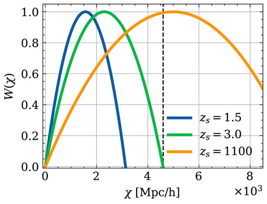
The lensing kernels of weak lensing convergence for three source redshifts.
Then each light-cone is made up of a set of discrete projected spherical density shells which are calculated by healpix9(Górski et al. 2005). We projected the dark matter particles to each shell at a comoving distance |$\chi$| using the snapshot with the nearest redshift (|$z_i \sim z(\chi)$|) to capture the evolution of redshift. According to Zorrilla Matilla et al. 2020, it is reasonable to fix projection depth at |$100~h {\rm Mpc}^{-1}$| for weak lensing survey. The healpix parameter |$N_\mathrm{side} = 8192$|, and the corresponding pixel resolution |$\Delta \theta =\sqrt{3/\pi }/N_{\text{side }} = 0.43~\mathrm{arcmin}$|.
Similar to Sgier et al. 2021, the convergence located in pixel |$\theta _\mathrm{pix}$| is given by the weighted summation of all lens planes along the line of sight
where |$N_{\mathrm{pix}}$| is the total number of pixels on the whole sky, |$V_{\text{sim }}$| is the volume of the simulation box, and |$N_\mathrm{p}$| is the total particle number in a cubic snapshot. For the ith lens plane, the projected number density |$n_{\mathrm{ p}}\left(\theta _{\mathrm{pix}}, \Delta \chi _{i}\right)$| should be weighted by the lensing kernel |$W_i(\chi _i, \chi _s)$|. Here, |$\chi _i = (2i-1)\Delta \chi /2$| and |$\chi _\mathrm{ s} = \chi (z_\mathrm{ s})$| are the comoving angular diameter distance of ith lens plane and source plane, respectively. It is crucial to emphasize that no randomization procedure is incorporated in the light-cone construction in this work. Nevertheless, in Appendix A, we additionally investigate two rotation strategies intended to mitigate repetitive structures.
In order to suppress the cosmic variance, we chose 25 different observers for the full-sky light-cone creation. All observer positions are generated by using Sobol sequence (Sobol’ 1967) to obey the Copernican principle.
3.2.2 Partial light-cone
To isolate the replication effects across various sky coverage areas, it is necessary to subdivide the full-sky convergence map into multiple sub-maps. Each sub-map should be centred along a distinct line-of-sight direction. To facilitate comparison, we first need to define the special and normal line-of-sight directions.
Based on the geometry of tiling, we can categorize three distinct types of special directions. They are the main axis directions (comprising 6 vectors denoted as |$(1,0,0) \times 6$|), the diagonal directions of the x–y/y–z/x–z planes (including 12 viewing angles notated as |$(1, 1, 0) \times 12$|), and the diagonal orientations of cubic boxes (containing 8 diagonal vectors notated as |$(1, 1, 1) \times 8$|). Since the identical large-scale structure manifests repeatedly along these three unique direction types, sub-maps aligned with these directions inherently exhibit notable box replication effects. To obtain a reliable conclusion, it is essential to include random lines of sight to serve as a baseline for comparison. We achieve this by uniformly dividing the entire celestial sphere into |$12N_\mathrm{side}^2$| directions, employing the ipix2vec function available in the healpix framework. For this study, we have chosen a value of |$N_\mathrm{side}= 4$|, resulting in 192 directions and associated sub-maps that serve as validation samples. Note that none of the 192 random directions overlaps with the three kinds of special directions. We call these validation samples as random light-of-sight samples although they are approximately uniformly distributed on the sphere. Additionally, it is essential to mention that the rotation of shell or shell bundles is not employed to remove the box replication effect since this process also changes the statistics slightly, as detailed in Appendix A.
In practice, the full-sky convergence map is rotated so that a specified line of sight is located at a specific angular position, i.e. |$\hat{n} = (\theta =0^{\circ }, \phi =0^{\circ }\mathrm{ degree}) = (1,0,0)$|. This is to avoid the high latitude projection effect from sphere to flat plane, and the equatorial zone can be pixelized to regular diamonds with minimal shape distortion by the healpix scheme. It is important to note that the rotation is performed in the spherical harmonic space to ensure the preservation of the lensing signal before and after rotation. Subsequently, we can extract the lensing signals in the vicinity of this particular direction using a square mask with an area of |$5\times 5~\ \mathrm{deg^2}$| as the fiducial case. The significance of the box replication effect is obviously dependent on the mask size. Thus, the different choices of mask size in this post-processing operation are also investigated in Section 4.4. We decrease the map resolution from |$0.43^{\prime \prime }$| to |$3.44^{\prime \prime }$| for a balance of speed and accuracy in the process.
4 RESULTS
In this section, we show the effects of the box-replication on the two-point statistics and high-order statistics.
4.1 Validation of full-sky convergence
Power spectrum and its counterpart, the two-point correlation function are widely used in cosmological analysis. First of all, we present the power spectra of the full-sky convergence maps in the top panel of Fig. 2. The red and blue lines represent the dimensionless power spectrum of weak lensing and CMB lensing, respectively. The black dotted lines indicate the results of equation (8), where the underlying density power spectrum is calculated by using |${\tt {CAMB}}$|10, which integrates the enhanced halo-model fitting formula, HMCODE, to offer accurate non-linear matter power spectrum predictions across various redshifts (Mead et al. 2015). To aid comparison, we display the ratio between simulation results and theoretical predictions in the bottom panel. The coloured region represents the standard deviation of the measurements from 25 realizations.
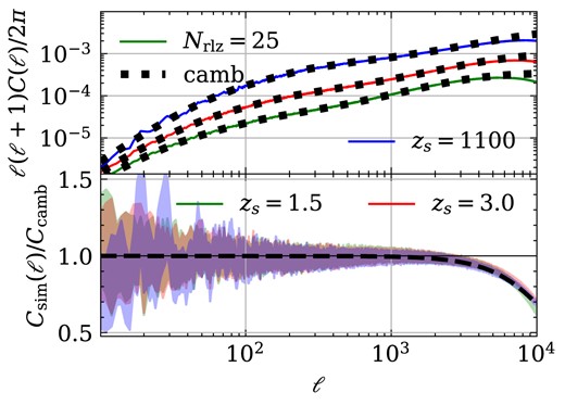
Top: validation of full-sky convergence power spectrum. The solid lines are from 25 realizations using Born approximation, while the thick dotted lines are the |${\tt {CAMB}}$| theoretical predictions from Limber integration. Bottom: we show the ratio between measurements and theoretical predictions. The shaded regions indicate the standard deviation of 25 different observers. The dashed line is determined using the formula outlined in equation 5 of Takahashi et al. 2017 by setting |$\ell _\mathrm{res} = 1.8 N_\mathrm{side}$| to describe the effect from limited resolution.
Our analysis reveals that the measured two-point statistics closely match the theoretical predictions for |$\ell \lesssim 2000$| across different source redshifts. At large scales (small |$\ell$|), the large scatter is caused by the sample variance. The remarkable agreement between the measured statistics and the theoretical predictions highlights the effectiveness of the Born approximation, a finding consistent with previous studies (e.g. Wei et al. 2018; Hilbert et al. 2020). The discrepancy observed between theoretical predictions and simulation results at angular scales |$\ell \gtrsim 2000$| primarily stems from the limited resolution of healpix maps. This effect can be approximately characterized by the equation provided in Takahashi et al. 2017:
where |$\ell _\mathrm{res} = 1.8 N_\mathrm{side}$|. This finding is consistent with the results of previous papers (e.g. Ferlito et al. 2023).
4.2 Partial sky convergence power spectrum
In this analysis, we compare the partial sky convergence power spectra of random samples with three distinct special directions. Here, the ‘partial sky’ means that we use a mask to highlight the presence of repeated structures. Because these artificial structures faded away quickly as the line of sight deviated from a particular direction. Similar to the previous figure, Fig. 3 shows the power spectrum of the masked convergence field for three different source redshifts, 1.5 (dotted), 3.0 (dashed), and 1100 (solid), obtained from the L1200 simulation. The black lines represent the computed mean spectra from |$25 \times 192$| realizations of partial light-cones along random viewing angles. In Appendix B, we demonstrate that employing the statistics from the aforementioned 192 random directions as a reference is appropriate, as the statistics from 768 directions and those from 128 safe directions with no-repetition (as discussed in later Section 5) is consistent with each other. Shaded regions are utilized to indicate the statistical error of the spectra. The results of three different types of special samples are presented in red, blue, and green data points, accompanied by the error bars depicting the measurement errors.
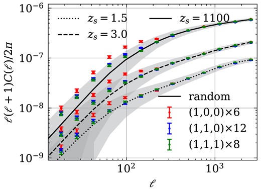
Convergence power spectrum of light-cones with an area of |$5 \times 5~\mathrm{deg}^2$| along random line-of-sight directions (solid, dashed and dotted lines) and three special kinds of orientations (data points). The shaded region indicates the standard deviations of 192 masked maps, while the data points and the error bars show the measurement errors of the power spectrum for special orientations.
Compared to the random samples, the first kind of special directions (red points) shows noticeable power spectrum excess at |$\ell \lesssim 200$|. Smaller overestimations can also be found for two other special directions (the blue and green data points). This could be attributed to the fact that the number of structure replications along these directions is less than the |$(1,0,0)\times 6$| directions. It is worth noting that the overestimated signals are observed for different source redshifts, suggesting that this effect is not strongly influenced by the specific kernel but rather is predominantly determined by the number of structure repetitions.
To further support our conclusion, we utilized the well-known cosmological simulation code, gadget-4 (as described in Springel et al. 2021), to generate an additional simulation. This simulation involved |$768^3$| particles evolved within a |$L=250^3~h^{-3} {\rm Mpc^3}$| box, enabling better visualization of the effects with low computational costs. With the on-the-fly light-cone code integrated into gadget-4, we were able to easily obtain full-sky density maps. By stacking the projected density fields with a thickness of |$25~h^{-1} \,{\rm Mpc}$| at different redshifts, we generated convergence maps that span the entire sky. We inspect the box-replication effect by showing the lensing convergence maps at |$\chi _\mathrm{ s} = N\times L$|, with |$N=3, 4, 6$|, and 8. Twelve maps are presented in Fig. 4 to provide visual representations for different N and different directions. These maps are also generated by selecting a |$5 \times 5~\mathrm{deg}^2$| region centred at (1, 0, 0), (1, 1, 0), and (1, 1, 1) direction. This visualization clearly shows us the artificial convergence structures depending on the special directions and the number of box repetitions. Note that |$N=3,4$| maps roughly have the same number of replications as the fiducial L1200 case at source redshift |$z_\mathrm{ s} = 1.5, 3.0$|, respectively. These artificial features extend to scale |$\theta \sim \pi /\ell \approx 1~\mathrm{deg}$|, explaining the power spectrum excess at |$\ell \lt 200$| in Fig. 3.
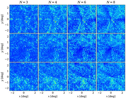
Visualization of partial sky convergence map of |$5\times 5~\mathrm{deg^2}$| using |$L=250~h^{-1} {\rm Mpc}$| simulation boxes. Different box repetition times N also indicate the distance of the source plane to the observer, |$\chi _\mathrm{ s}=250N~h^{-1} {\rm Mpc}$|. The stacking of partial sky light-cones along the most special direction (1, 0, 0) is shown in the upper panels. The middle and lower panels represent the sky area with the same size as the upper panels but for the line-of-sight direction |$(1, 1, 0)$| and (1, 1, 1), respectively. Note that for our case using L1200 simulation, |$N \approx 2.6,\ 3.8$| for |$z_\mathrm{ s} = 1.5,\ 3.0$|, respectively.
4.3 Convergence moments
After the investigation of the power spectrum, it is natural to inquire whether the box replication effect has a more pronounced influence on higher order statistics. Moments of smoothed lensing fields can capture the non-Gaussianity, and definitely will be affected by the non-Gaussian artificial structures appear in Fig. 4. We smooth the convergence field first and then again apply the mask to pick out a |$5\times 5~\mathrm{deg^2}$| region for a given line of sight. The moments here are less affected by the detailed shape of the mask by definition. We present the higher order moments of the smoothed convergence fields for different lensing kernels and line-of-sight directions in Fig. 5. For the lowest source redshift case, the box replication effect on all statistics is below the statistical uncertainty because of the small times of structure repetition |$N \sim 2.6$|. For higher source redshifts, second-order and fourth-order moments are effective in distinguishing |$(1,0,0) \times 6$| directions and random viewing angles. For the other two special orientations, the box replication effect has much lower significance. This can be attributed to the relatively small repetition times of |$N \sim 3.8$|. The kaleidoscopic structures resulting from box tiling appear to be less prominent when |$N \lesssim 4$|. All these findings are consistent with the power spectra analysis in the previous section. Moreover, a comparison can be made between the upper panels and the bottom panels in Fig. 5. Larger deviations are observed for both the second-order and fourth-order moments of CMB lensing convergence. We argue that this is primarily due to the monotonically slowly increasing CMB lensing kernels at low redshifts, as shown in Fig. 1.
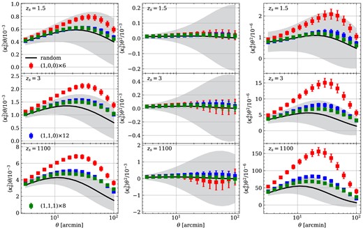
Left: second-order moments of |$25~\mathrm{deg^2}$| convergence fields with different smoothing scales. The results of the source galaxy at |$z_\mathrm{ s}=1.5, 3.0$| are shown in the top and middle panels, respectively. Meanwhile, the CMB lensing fields at |$z_\mathrm{ s}=1100$| are shown in the bottom panel. Middle: third-order moments of the smoothed lensing fields. Right: fourth-order moments of the smoothed weak lensing and CMB lensing convergence maps.
Surprisingly, when considering third-order moments of smoothed fields alone, it becomes challenging to distinguish between the special directions. The box replication effect can create both denser regions and deeper voids in the lensing convergence. As a result, this symmetry makes the skewness of |$\kappa$| less affected.
4.4 Mask size
In this section, we focus on the mask size in the partial sky light-cone construction detailed in Section 3.2.2. A larger mask will cover more normal regions, and dilute the significance of the box replication effect. To address this concern, we vary the sky size from |$25~\mathrm{deg^2}$| to |$400\ \mathrm{deg^2}$| and compute all four statistics for three distinct types of specialized viewing angles, subsequently comparing them to the results obtained from random sampling. For the partial sky convergence spectrum, we show the normalized |$\hat{C}(\ell) = C(\ell)/ A_{\rm sky}$| at |$\ell = 100$| where |$A_{\rm sky}$| represents the area of sky coverage. The smoothing scale of the lensing fields remains fixed at |$29~\mathrm{arcmin}$| throughout this analysis, as from Fig. 5 at this smoothing scale the deviation is larger than other scales.
All results are shown in Fig. 6. When the sky coverage is limited, the measurements of moments exhibit noticeable deviations from the expected values. This deviation is even more pronounced for the data points associated with CMB lensing when compared to low redshift sources. The trend for different lensing kernels is consistent with the previous conclusion in Section 4.3. However, as the sky coverage increases to |$400~\mathrm{deg^2}$|, no significant difference is observed among the various light-cones with different lensing kernels and viewing angles. This is caused by the decreasing ratio of special areas to total areas when increasing the mask size. This effect can be statistically insignificant for the Stage-III surveys with a few thousand square degrees sky coverage if the simulation volume is sufficiently large (|${\gtrsim} 0.2 h^{-3} \,{\rm Gpc^3}$|).11 We point out that this dilution in statistics does not mean the systematic features have vanished in special directions. Therefore, when analysing local estimators like peaks and minima, additional caution is required.
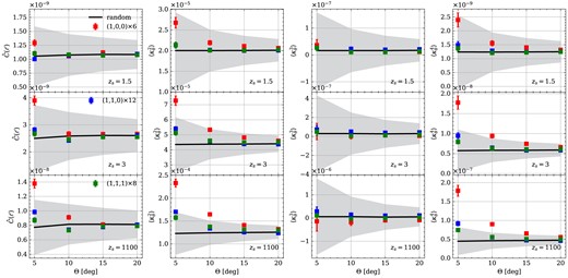
First column: normalized partial sky convergence power spectrum at |$z_\mathrm{ s} = 1.5,\ 3.0$| and 1100. The horizontal axis indicates the patch size. The measurements of galaxy lensing are presented in the top panel. The results of CMB lensing are shown in the bottom panel. Second column: second-order moments of partial sky convergence fields within different areas. Third column: third-order moments of the smoothed lensing fields. Fourth column: fourth-order moments of the smoothed weak lensing and CMB lensing convergence maps.
Fig. 6 also implies that the box replication effect diminishes rapidly when the line of sight deviates from certain specific directions. This suggests that this artificial effect can be avoided as long as we keep away from almost special directions during the light-cone construction. Therefore, the final problem lies in identifying the directions that give rise to the box replication effect. We will discuss how to build a robust light-cone by achieving this in Section 5.
4.5 Bayesian tension metric
To account for the influence of systematic effects on the theoretical modelling, we adopt a parameter-fitting approach to translate these effects into constraints on cosmological parameters. We achieve this by fitting the statistics obtained from the random line-of-sight directions, each with minimized box replication effects, using a univariate model of the form |$\boldsymbol{d} = A\boldsymbol{d}_{\rm model}$|. In this model, |$\boldsymbol{d}$| represents the measured statistic obtained from each random sample, while |$\boldsymbol{d}_{\rm model}$| corresponds to the mean estimation derived from each type of special orientation. The parameter A allows for the quantification of the systematic effects on the observed statistics and their impact on the cosmological parameter constraints. By fitting this model to the data, we can better understand and account for the systematic uncertainties in the theoretical modelling process.
Under the Gaussian distribution assumption, the A parameter is minimized by
We can easily obtain the best-fitting parameter by an analytic formula:
Here, |$N_{\ell /\theta }$| represents the number of data points for the convergence power spectrum and moments. We use a conservative scale limit at |$30 \le \ell \le 1000$| with |$N_{\ell } = 20$|. It is worth noting that for Stage-IV surveys, such as those discussed in Yao et al. 2023, the scale range will extend to |$\ell _{\rm max} \sim 3000$|, which further reduces the influence of box replication effects due to the inclusion of smaller scales. For the latter statistics, the smoothing angles are fixed at |$[3.2, 100]~\text{arcmin}$| with |$N_{\theta }=14$|.
Table 1 depicts the outcomes obtained from the analysis of light-cones with a sky coverage of |$5\times 5~\mathrm{deg^2}$|. Our findings reveal that the systematic bias resulting from the box replication effects remains smaller than the statistical error, with the exception of the fourth convergence moments of light-cones along the most exceptional direction, denoted as (1,0,0). Considering the increasing sky coverage of modern galaxy surveys, we have included the results obtained from a |$400~\mathrm{deg^2}$| mask in Table 2. Remarkably, when considering the correlation between different scales and statistical errors in our analysis, the influence of the box replication effect on the four lensing statistics can be well controlled. This moderate impact can be attributed to the dilution of typical regions as the sky coverage expands. However, these repeated structures persist within these special directions, potentially giving rise to extra angular correlations for other statistics, e.g. peaks, minima, and Minkowski functionals. We leave this for future investigation.
The parameter A fitting results for |$5\times 5~\mathrm{deg^2}$| partial sky light-cones with three different source redshifts and three kinds of line-of-sight directions. |$\frac{|\langle A \rangle -1|}{\sigma (A)}$| can be utilized to quantify the systematic bias in the modelling, where |$\langle A \rangle$| is the average value of A and |$\sigma (A)$| is the standard deviation of A. We use bold font to highlight the bias larger than |$0.5 \sigma$|.
| Direction | (1,0,0) | (1,1,0) | (1,1,1) | |||||||
|---|---|---|---|---|---|---|---|---|---|---|
| statistics | |$\langle A\rangle$| | |$\sigma (A)$| | |$\frac{|\langle A\rangle -1|}{\sigma (A)}$| | |$\langle A\rangle$| | |$\sigma (A)$| | |$\frac{|\langle A\rangle -1|}{\sigma (A)}$| | |$\langle A\rangle$| | |$\sigma (A)$| | |$\frac{|\langle A\rangle -1|}{\sigma (A)}$| | |
| |$C_{\kappa \kappa }(\ell)$| | |$z_\mathrm{ s} = 1.5$| | 0.974928 | 0.115627 | 0.216835 | 1.006055 | 0.118281 | 0.051191 | 0.984959 | 0.115710 | 0.129985 |
| |$z_\mathrm{ s} = 3.0$| | 0.976937 | 0.080271 | 0.287318 | 1.001877 | 0.081253 | 0.023103 | 0.993261 | 0.080433 | 0.083779 | |
| |$z_\mathrm{ s} = 1100$| | 0.959066 | 0.060307 | 0.678757 | 0.992844 | 0.061867 | 0.115666 | 0.994603 | 0.061910 | 0.087167 | |
| |$\langle \kappa ^2_{\theta } \rangle$| | |$z_\mathrm{ s} = 1.5$| | 0.983280 | 0.089468 | 0.186883 | 1.034505 | 0.093977 | 0.367162 | 0.985125 | 0.089406 | 0.166378 |
| |$z_\mathrm{ s} = 3.0$| | 0.979632 | 0.061898 | 0.329055 | 1.020842 | 0.064245 | 0.324409 | 0.989774 | 0.062255 | 0.164258 | |
| |$z_\mathrm{ s} = 1100$| | 0.980437 | 0.039573 | 0.494358 | 1.017404 | 0.040917 | 0.425351 | 0.993138 | 0.039938 | 0.171823 | |
| |$\langle \kappa ^3_{\theta } \rangle$| | |$z_\mathrm{ s} = 1.5$| | 0.988661 | 0.255906 | 0.044309 | 1.076210 | 0.277321 | 0.274809 | 0.980875 | 0.253020 | 0.075588 |
| |$z_\mathrm{ s} = 3.0$| | 0.987609 | 0.236556 | 0.052382 | 1.063988 | 0.251966 | 0.253955 | 0.968756 | 0.229322 | 0.136244 | |
| |$z_\mathrm{ s} = 1100$| | 0.910621 | 0.244983 | 0.364838 | 1.038345 | 0.271368 | 0.141303 | 0.940633 | 0.246464 | 0.240873 | |
| |$\langle \kappa ^4_{\theta } \rangle$| | |$z_s = 1.5$| | 0.668164 | 0.393678 | 0.842912 | 0.983395 | 0.533746 | 0.031109 | 0.945442 | 0.505685 | 0.107890 |
| |$z_\mathrm{ s} = 3.0$| | 0.568817 | 0.212749 | 2.026718 | 0.920131 | 0.300942 | 0.265396 | 0.916459 | 0.295385 | 0.282819 | |
| |$z_\mathrm{ s} = 1100$| | 0.683477 | 0.126141 | 2.509281 | 0.950014 | 0.156286 | 0.319838 | 0.924932 | 0.151501 | 0.495497 | |
Same as Table 1, but for a larger sky coverage of |$20\times 20~\mathrm{deg^2}$|.
| Statistics | |$\langle A\rangle$| | |$\sigma (A)$| | |$\frac{|\langle A\rangle -1|}{\sigma (A)}$| | |$\langle A\rangle$| | |$\sigma (A)$| | |$\frac{|\langle A\rangle -1|}{\sigma (A)}$| | |$\langle A\rangle$| | |$\sigma (A)$| | |$\frac{|\langle A\rangle -1|}{\sigma (A)}$| | |
|---|---|---|---|---|---|---|---|---|---|---|
| |$C_{\kappa \kappa }(\ell)$| | |$z_\mathrm{ s} = 1.5$| | 1.001167 | 0.032916 | 0.035461 | 1.001257 | 0.032919 | 0.038179 | 1.001737 | 0.032935 | 0.052733 |
| |$z_\mathrm{ s} = 3.0$| | 0.998582 | 0.021475 | 0.066038 | 1.002398 | 0.021557 | 0.111239 | 1.001749 | 0.021543 | 0.081178 | |
| |$z_\mathrm{ s} = 1100$| | 0.996026 | 0.015926 | 0.249513 | 1.003449 | 0.016043 | 0.215014 | 1.001949 | 0.016020 | 0.121639 | |
| |$\langle \kappa ^2_{\theta } \rangle$| | |$z_\mathrm{ s} = 1.5$| | 0.996121 | 0.026283 | 0.147605 | 1.011579 | 0.026692 | 0.433797 | 1.002197 | 0.026442 | 0.083106 |
| |$z_\mathrm{ s} = 3.0$| | 0.996252 | 0.017760 | 0.211046 | 1.008455 | 0.017977 | 0.470342 | 1.001049 | 0.017845 | 0.058763 | |
| |$z_\mathrm{ s} = 1100$| | 0.995009 | 0.011963 | 0.417200 | 1.008072 | 0.012119 | 0.666113 | 1.000064 | 0.012023 | 0.005318 | |
| |$\langle \kappa ^3_{\theta } \rangle$| | |$z_\mathrm{ s} = 1.5$| | 0.980255 | 0.065672 | 0.300657 | 1.021229 | 0.068395 | 0.310396 | 1.007512 | 0.067477 | 0.111333 |
| |$z_\mathrm{ s} = 3.0$| | 0.981669 | 0.059531 | 0.307918 | 1.019302 | 0.061784 | 0.312419 | 1.003599 | 0.060840 | 0.059156 | |
| |$z_\mathrm{ s} = 1100$| | 0.977213 | 0.063501 | 0.358842 | 1.018759 | 0.066143 | 0.283610 | 0.993324 | 0.064492 | 0.103513 | |
| |$\langle \kappa ^4_{\theta } \rangle$| | |$z_\mathrm{ s} = 1.5$| | 0.965330 | 0.134665 | 0.257456 | 1.014115 | 0.141257 | 0.099921 | 1.019490 | 0.142071 | 0.137184 |
| |$z_\mathrm{ s} = 3.0$| | 0.977436 | 0.084264 | 0.267779 | 1.012450 | 0.087022 | 0.143068 | 1.009962 | 0.086910 | 0.114628 | |
| |$z_\mathrm{ s} = 1100$| | 0.989491 | 0.041604 | 0.252600 | 1.014702 | 0.042586 | 0.345230 | 1.002519 | 0.042102 | 0.059836 |
A recent frequently used convergence field construction scheme is to put the observer at the box corner and keep the octant sky light-cone (e.g. Korytov et al. 2019; Hadzhiyska et al. 2023; Hernández-Aguayo et al. 2023; Euclid Collaboration 2024). Upon examining the two tables, we observe that the standard deviation of A, denoted by |$\sigma (A)$|, exhibits an inverse square root dependence on the sky coverage, satisfying the expectation from a statistical view. Furthermore, the systematic bias, indicated by |$|\langle A \rangle -1|$|, decreases with the increasing area if no additional special regions are introduced. Taking into account the very limited spatial extent of kaleidoscope-like structures and the large fraction of the normal regions, we expect that the systematic bias associated with a single octant light-cone will be significantly reduced compared to the values presented in Table 2.
Obviously, the systematic bias induced by the kaleidoscope-like structures depends on the number of box replications N, or equivalently the size of the simulation box used to tile the light-cone. The weak lensing statistics at higher redshift are expected to suffer more from the box replication effect. However, the measured |$\langle A \rangle$| is roughly the same for two source redshifts |$z_\mathrm{ s} = 1.5$| and 3.0 for given statistics and sky coverage in Tables 1 and 2. This coincidence is attributed to two factors, an increased lensing signal at a high source redshift and an increased systematic bias at a high source redshift. From Fig. 4, we can find that some kaleidoscope feature is composed of a string of radial halo-like structures. This is a direct consequence of the same halo observed at different redshifts. They will all contribute to the |$\kappa$| moments if the smoothing length is comparable to the scale of these string-like structures. Naively, the amplitude of bias on |$\kappa$| is roughly proportional to an effective N when the lensing kernel is taken into account,
Here, |$W_\mathrm{max}$| is the maximum value of the lensing kernel. For CMB lensing at |$z_\mathrm{ s}=1100$| and weak lensing at |$z_\mathrm{ s}=3$|, the simulation boxes employed in the light-cone construction in this work are the same. The larger bias that appeared in CMB lensing cases is due to the relatively flat lensing kernel, leading to |$N_\mathrm{eff}=0.756N$| compared to the weak lensing result |$N_\mathrm{eff}=0.625N$|, with |$N=3.833$|.
5 LINE-OF-SIGHT FINDER
As discussed in previous sections, it has been established that stacking along the special angles [especially for |$(1,0,0)\times 6$|] leads to artificial structures and obvious systematic errors in higher order lensing statistics for light-cones with a small coverage. Fortunately, this effect fades away quickly as indicated in Section 4.4. This finding allows us to identify alternative special directions that can be explored to minimize the occurrence of excessive box replications.
It is easy to understand that the box replication effect dominates by the times of structure repetitions. Therefore, we use particles placed on uniform grids to represent small volumes encompassing the entire box. Then, the box is stacked through regular repetition, and the particles are projected onto the lens plane based on a specified light-cone geometry. Here, we employ the healpix scheme to pixelize the entire sky for a given |$N_\mathrm{side}$|. In the final step, it is crucial to record the number of appearances for each particle in each pixel. Since each particle represents a small volume around its position, this allows us to interpret the number of appearances, denoted as n, as the number of structure repetitions. We define the unique index |$I = N(n=1)/N(n\ge 1)$| as the quantitative indicator of the box replication effect. Here, N is the number of structures appearing n times in the stacking process. A unique light-cone is characterized by a value of one for I in a given pixel, indicating the absence of the box replication effect for that particular sky coverage. To facilitate accessibility, we have made the code publicly available for further exploration and utilization at https://github.com/czymh/losf.
By implementing this pipeline, we can conveniently divide the entire sky into 768 pieces uniformly with |$N_\mathrm{side}= 8$|. The unique indices corresponding to each piece are presented in Fig. 7. The light-cone geometry employed here aligns with the convergence map construction of the L1200 simulation. The underlying test particle number on each dimension is 10. We also increase this number to 100 and obtain the converged result. In this case, there are 128 unique light-cones, and the total sky coverage amounts to |$6875~\mathrm{deg^2}$|. Notably, the directions characterized by high repetition times, indicated by the blue region in the figure, are primarily concentrated around three distinct types of special directions. This is also consistent with our previous findings, further supporting our earlier analysis and conclusions.
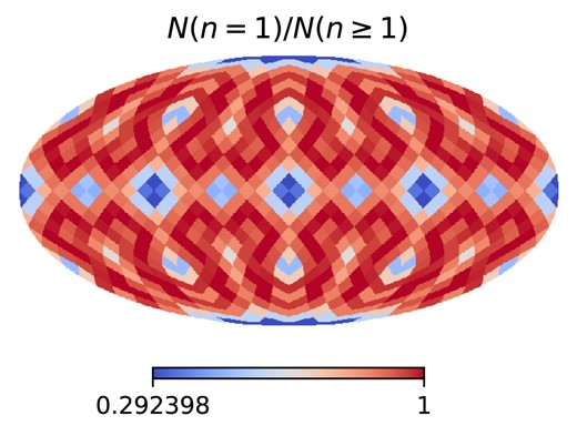
The full-sky unique index map for |$N_\mathrm{side}=8$|. Each pixel represents a pencil-beam light-cone whose sky coverage is about |$54~\mathrm{deg^2}$|.
6 CONCLUSIONS
Within the scope of this study, we have examined the influence of the box replication effect on convergence power spectra and high-order moments of lensing fields. The origin of this effect can be traced back to the finite simulated volume, thereby impacting both post-processing and on-the-fly light-cone constructions.
To satisfy the requirement of Stage-IV surveys, we used the high-resolution N-body simulation evolving |$3072^3$| particles with large box sizes |$1.2\ h^{-1}\, {\rm Gpc}$| to construct light-cones along different directions by tiling the simulation boxes. The measurements of convergence power spectra and higher order moments of the light-cones along three kinds of special orientations are compared with the results of random line-of-sight directions in Section 4. For small patch size |$25~\deg ^2$|, noticeable deviations can be observed in the power spectrum at |$\ell \ \lt\ 200$|, as well as in second- and fourth-order moments for |$z_\mathrm{ s}=3$| and 1100. However, the impact of the box replication effect remains confined within the bounds of statistic error for these statistics with |$z_\mathrm{ s} = 1.5$|, as shown in Figs 3 and 5. The visual inspection reveals that the tessellation geometry employed in weak gravitational lensing simulations can introduce kaleidoscopic structures, particularly in directions where multiple copies of the simulation box are present at high source redshifts.
To assess the systematic bias in weak lensing statistics, a univariate model is utilized to fit estimations obtained from random samples to measurements derived from light-cones oriented towards specific viewing angles. Significant bias arising from the aforementioned repeated structures is observed primarily in the fourth-order moments of smoothed CMB lensing convergence fields. However, this bias diminishes below the level of statistical errors as the size of the mask is increased from |$25$| to |$400~\mathrm{deg^2}$|. Consequently, it is concluded that the impact of the box replication effect on the four lensing statistics is statistically insignificant for Stage-III and Stage-IV surveys when employing current dark matter simulations featuring a box size of |$L \gtrsim 600 h^{-1} \,{\rm Mpc}$|. None the less, this effect becomes significant because of the extended box replication time N for the simulation with |$L \lesssim 250 h^{-1} \,{\rm Mpc}$|, a prevalent choice for hydrodynamic simulations. Given the presence of repeated structures along special directions, caution is advised when evaluating high-order statistics derived from light-cones with limited sky coverage.
In such instances, these artificial features rapidly vanish when the viewing angles deviate from specific directions, as indicated in Fig. 6. Thus, unbiased construction of light-cones can be achieved by avoiding these particular lines of sight. We developed a code to find the unique light-cones to avoid structure repetition spanning the whole sky and make it publicly available. In summary, the box replication effect is trivial for generating a mock of the current galaxy survey (effectively |$z_\mathrm{ s} \sim 1.5$|) through cosmological simulation with a large box (|$L \gtrsim 600~h^{-1} {\rm Mpc}$|; e.g. Sgier et al. 2021; Ferlito et al. 2023; Kacprzak et al. 2023; Broxterman et al. 2024; Omori 2024).
For the purpose of precision cosmological constraints, the box replication effect on the covariance of different lensing statistics should also be quantified well. The generation of multiple realizations of lensing convergence maps is indeed necessary for estimating covariance matrices precisely. Therefore, we defer this task to future investigation. Another possible extension of this work is to investigate the box replication effect on other statistics, especially for some morphological tools, i.e. Minkowski functionals. The incorporation of novel statistical methodologies should facilitate a more comprehensive modelling of these anomalous artificial features.
ACKNOWLEDGEMENTS
We thank Pengjie Zhang for the useful discussions. This work was supported by the National Key R&D Program of China (2023YFA1607800 and 2023YFA1607802), the National Science Foundation of China (grant number 12273020), the China Manned Space Project with number CMS-CSST-2021-A03, the ‘111’ Project of the Ministry of Education under grant number B20019, and the sponsorship from the Yangyang Development Fund. This work made use of the Gravity Supercomputer at the Department of Astronomy, Shanghai Jiao Tong University.
DATA AVAILABILITY
All data included in this study are available upon reasonable request by contacting the corresponding author.
Footnotes
The corresponding side length of the simulation box is |${\sim} 600~h^{-1} \,{\rm Mpc}$|, which only reaches four times box replications for galaxy catalogue at a |$z\sim 1$|. This should increase according to the redshift distribution for the future survey.
REFERENCES
APPENDIX A: RANDOMIZATION PROCEDURE
In this appendix, we examine the impact of three different rotation strategies on the convergence power spectrum.
No Rotation: no rotation is applied to each mass shell which is our fiducial choice in the main text.
Box Rotation: shells are randomly rotated in bundles of a box length |$1200~h^{-1} {\rm Mpc}$|.
Shell Rotation: each mass shell undergoes a random rotation to mitigate repeated structures in the light-cone construction.
The mass shells pixelated by healpix are rotated in the spherical harmonic space rather than rotating the particles directly to save computational cost. To reduce cosmic variance, we generate 25 realizations for each of the three methods.
Fig. A1 illustrates the ratios of full-sky convergence power spectrum and moments for these strategies relative to no-rotation results at three source redshifts. In the first to fourth columns, the results of the power spectrum, second-order moments, third-order moments, and fourth-order moments are shown in sequence. Correspondingly, from the first to the third rows, the data for the source redshifts at 1.5, 3.0, and 1100 are exhibited in turn. The mean measurement and statistical error of no rotation results is shown by the blue shadow. In contrast, the rotation of every box length and the rotation of each individual shell are indicated by green and yellow circles, respectively.
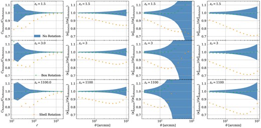
The impact of three rotation strategies on four statistics for source galaxies at |$z_\mathrm{ s} = 1.5, 3.0, 1100$|. The first to fourth columns present the results of the power spectrum, second-order moments, third-order moments, and fourth-order moments, respectively. The statistical uncertainty from 25 non-rotation light-cones is shown by the shaded region. The circles denote for the rotated shells for every box length, and for each rotated shell.
For the power spectrum, the approximately 2 per cent suppression at |$\ell \lesssim 100$| introduced by the second rotation strategy is negligible compared to cosmic variance. However, for second and fourth-order moments, we observe that this strategy induces |$1\sigma$| level deviations for |$\theta \lt 10~^\prime$|. Rotating each mass shell in the light-cone construction has a considerable impact on large scales for all statistics. The power spectrum result here is consistent with Upadhye et al. (2024). The more times of rotations in this method result in a greater loss of correlation between different mass shells. Given that the rotation changes the amplitude of the high-order moments comparable to the statistical uncertainty at small scales, we do not utilize the rotation method to set the reference.
APPENDIX B: VALIDATION OF RANDOM SAMPLE
In Section 4, we treat the light-cones towards 192 random angles as the fiducial sample where the box replication effects are minimized, though some still suffer from repeated structures. The reliability of this approach needs examination. Fortunately, we can obtain 128 unique light-cones by implementing the pipeline with |$N_\mathrm{side} = 8$| described in Section 5. Although the geometrical configuration of the healpix pixel differs from the mask utilized by us, the area of a single pixel, which is |$53.7~\mathrm{deg^2}$|, can cover the mask. Moreover, a more uniform sample is generated by splitting the whole sky into 768 directions. Four statistics of three random samples are shown in Fig. B1. The statistical means and errors are all consistent, indicating that our fiducial choice is reliable.
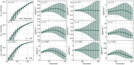
Convergence power spectrum and moments of three random samples. To enhance visualization, we multiplied the x-axis variables of the 768 samples by 1.1. The three random samples are statistically indistinguishable.
