Understanding the phenomenological and intrinsic blazar sequence using a simple scaling model

ABSTRACT

The blazar sequence, including negative correlations between radiative luminosity L_rad and synchrotron peak frequency ν, and between Compton dominance Y and ν, is widely adopted as a phenomenological description of spectral energy distributions (SEDs) of blazars, although its underlying cause is hotly debated. In particular, these correlations turn positive after correcting Doppler boosting effect. In this work, we revisit the phenomenological and intrinsic blazar sequence with three samples, which are historical sample (SEDs are built with historical data), quasi-simultaneous sample (SEDs are built with quasi-simultaneous data) and Doppler factor corrected sample (a sample with available Doppler factors), selected from literature. We find that phenomenological blazar sequence holds in historical sample, but does not exist in quasi-simultaneous sample, and intrinsic correlation between L_rad and ν becomes positive in Doppler factor corrected sample. We also analyse if the blazar sequence still exists in subclasses of blazars, i.e. flat-spectrum radio quasars and BL Lacertae objects, with different values of Y. To interpret these correlations, we apply a simple scaling model, in which physical parameters of the dissipation region are connected to the location of the dissipation region. We find that the model generated results are highly sensitive to the chosen ranges and distributions of physical parameters. Therefore, we suggest that even though the simple scaling model can reproduce the blazar sequence under specific conditions that have been fine-tuned, such results may not have universal applicability. Further consideration of a more realistic emission model is expected.

radiation mechanisms: non-thermal, galaxies: active, galaxies: jets

1 INTRODUCTION

Blazars are the most extreme active galactic nuclei (AGNs) with relativistic jets aligned to our line of sight (Urry & Padovani 1995). The spectral energy distribution (SED) of blazars consists of two broad non-thermal emission components in the log ν−log νL_ν diagram. The low-energy component, peaking between the infrared to X-ray bands, is believed to originate from the synchrotron emission of relativistic electrons within the jet. The high-energy component, peaking in the γ-ray band, is believed to originate from the inverse Compton (IC) emission of the same electron population that up-scatter, either the synchrotron photons emitted by the same population of relativistic electrons (synchrotron self-Compton, SSC; Konigl 1981) or external photons (external Compton, EC; Ghisellini & Maraschi 1989; Dermer, Schlickeiser & Mastichiadis 1992; Dermer & Schlickeiser 1993; Sikora et al. 2002) from an accretion disc, a broad-line region (BLR), or a dusty torus (DT). Based on the equivalent width (EW) of the emission lines, blazars are divided into flat-spectrum radio quasars (FSRQs) with strong broad emission lines (EW > 5 Å), and BL Lacertae objects (BL Lacs) with absent or weak emission lines (EW ≤ 5 Å; Marcha et al. 1996; Landt et al. 2004; Xiong & Zhang 2014). Ghisellini et al. (2011) introduce a physical distinction between these two subclasses based on the BLR luminosity L_BLR in units of the Eddington luminosity L_Edd of the central supermassive black hole (SMBH). FSRQs are objects whose L_BLR ≳ 5 × 10⁻⁴L_Edd, and BL Lacs are the others. In addition to the FSRQs and BL Lacs classification, Abdo et al. (2010a) divide blazars into high-synchrotron-peaked (HSP) blazars if their synchrotron peak |$\nu _{\rm s}^{\rm p}\gt 10^{15}~\rm Hz$|⁠, intermediate-synchrotron-peaked (ISP) blazars if their synchrotron peak |$10^{14}~\rm Hz\lt \nu _{\rm s}^{\rm p}\lt 10^{15}~\rm Hz$| and low-synchrotron-peaked (LSP) blazars if their synchrotron peak |$\nu _{\rm s}^{\rm p}\lt 10^{14}~\rm Hz$|⁠.

Based on a sample of 126 blazars, Fossati et al. (1998) identified that their observed radiative luminosity, and the Compton dominance (the ratio of fluxes or luminosities of high- and low-energy components) are both anticorrelated to the observed synchrotron peak frequency. These two negative correlations are referred to as the well-known ‘blazar sequence’. The first physical explanation is proposed by Ghisellini et al. (1998). They suggested that if the intrinsic jet power is connected to L_BLR, one would expect the synchrotron peak frequency shifts from high frequency to low frequency by increasing the intrinsic jet power and increasing the radiative cooling dominated by the EC scattering. If this interpretation is correct, it provides a powerful tool for understanding the evolution of blazars’ SEDs, similar to the evolution of stars on the Hertzsprung–Russel diagram. Theoretical models suggest that the jet power is generated from accretion and the extraction of rotational energy or angular momentum from the disc/black hole (Blandford & Znajek 1977; Blandford & Payne 1982); therefore, the jet properties and emissions are linked to the black hole mass and accretion rate. Ghisellini & Tavecchio (2008) further highlight that the black hole mass and accretion rate are connected to the jet power and the shape of SED, providing a framework that could help explain the existence of both low-luminosity ‘blue’ quasars and low-luminosity ‘red’ quasars. The importance of the accretion rate is also pointed out by Meyer et al. (2011). They find that AGNs in the blazar sequence diagram is mainly composed of two groups, the primary difference between these groups being the accretion rate. The group with a high accretion rate consists mostly of LSP blazars and FR II radio galaxies, while the group with a low accretion rate corresponds to the majority of BL Lacs and FR I radio galaxies. In addition, many other studies endeavor to come up with physical interpretations of the blazar sequence. For instance, Böttcher & Dermer (2002) propose a simple analytical model, suggesting that the reduction of gas and dust in external environment causes the evolutionary sequence from FSRQ to BL Lacs-LSPs, and then to BL Lacs-HSPs. Björnsson (2010) propose that the blazar sequence can be well understood in the case of multiple IC scatterings, and the energy density of relativistic electrons is the main factor influencing the formation of the blazar sequence. Finke (2013) construct a simple model to explain the blazar sequence in the 2LAC clean sample, suggesting that the difference between sources is associated with the magnetic field of the jet’s dissipation region, the energy density of the external photon field, and the jet’s viewing angle. Note that all sources in the modelling are assumed to have the same bulk Lorentz factor. Potter & Cotter (2013b) propose a relativistic continuous jet model, which suggests that the blazar sequence could be interpreted if the radius of the transition region and bulk Lorentz factor of the jet increase with the jet power. According to their interpretation, FSRQs have large bulk Lorentz factors, and scatter external cosmic microwave background photons at large distances, resulting in larger Compton dominance and lower IC peak frequency. On the other hand, BL Lacs, which have lower jet powers, possess stronger magnetic fields in the bright synchrotron transition region compared to high-power FSRQs, leading to higher peak frequency synchrotron and SSC emissions.

Since the discovery of the blazar sequence, its underlying cause and if it is a result of selection effect have been widely discussed, but even so it is still frequently adopted as a description of the blazar population. With the improvement of detector sensitivity and the expansion of samples, the blazar sequence has been confirmed and developed (Ghisellini & Tavecchio 2008; Chen & Bai 2011; Finke 2013; Xiong et al. 2015a; Ghisellini 2016; Mao et al. 2016; Ghisellini et al. 2017; Savard, Ruan & Haggard 2022; Kerby & Falcone 2023; Ouyang et al. 2023). Finke (2013) suggests that the redshift selection effect cannot explain the blazar sequence. In Ghisellini et al. (2017), a revised version of the blazar sequence, named the ‘Fermi blazar sequence’, is propose by using a clean sample of 747 blazars (299 BL Lacs and 448 FSRQs) from the third catalogue of AGN detected by Fermi-LAT (Ackermann et al. 2015). In this large blazar sample, the existence of the blazar sequence is confirmed. However it is also pointed out that when considering BL Lacs and FSRQs separately, the sequence still holds for BL Lacs but not for FSRQs. On the other hand, the blazar sequence is questioned by the discovery of ‘outlier’ blazars (e.g. luminous HSP blazars) and the evidence of selection effects (Nieppola, Tornikoski & Valtaoja 2006; Padovani, Giommi & Rau 2012; Giommi et al. 2012a, b; Giommi & Padovani 2015; Raiteri & Capetti 2016; Cerruti et al. 2017; Keenan et al. 2021).

In the original physical interpretation (Ghisellini et al. 1998), radiative cooling is suggested as the main cause of the two negative correlations in the phenomenological blazar sequence. If so, these two negative correlations should firstly hold in the comoving frame; therefore, it has to be assumed that all blazars have similar values of the Doppler factor, or the Doppler factor is not related to other physical parameters (Ghisellini et al. 2017; Prandini & Ghisellini 2022). However, some studies argue that the phenomenological blazar sequence is an artefact of the Doppler boosting, since these two correlations with Doppler-corrected values turn positive or disappear (Landt & Bignall 2008; Nieppola et al. 2008; Wu, Gu & Jiang 2009; Xiong et al. 2015b; Fan, Bai & Mao 2016a; Fan et al. 2017; Chen et al. 2021; Yang et al. 2022b). It poses a challenge to the physical understanding of the blazar sequence.

In this work, we are motivated to revisit the phenomenological and intrinsic blazar sequence of samples in the literature, and propose a theoretical interpretation to these correlations. In previous studies, the blazar sequence is studied with historical SEDs. However, since blazars are highly variable objects, we also check if the blazar sequence holds for the quasi-simultaneous SEDs. This paper is organized as follows. In Section 2, we revisit the blazar sequence with three samples. In Section 3, we propose a theoretical consideration to understand the phenomenological and intrinsic blazar sequence. Finally, we end with the conclusion in Section 4. Throughout the paper, the cosmological parameters |$H_{0}=69.6\ \rm km\ s^{-1}\, Mpc^{-1}$|⁠, Ω₀ = 0.29, and Ω_Λ= 0.71 are adopted (Bennett et al. 2014).

2 REVISITING THE BLAZAR SEQUENCE WITH THE Fermi BLAZAR

The original blazar sequence is a phenomenological description of the blazars’ SED, including the negative correlations between the synchrotron peak frequency and the radiative luminosity, and between the synchrotron peak frequency and Compton dominance. In this section, we revisit these two correlations both in the observers’ frame and in the comoving frame with different samples.

When studying the correlation between the radiative luminosity and the synchrotron peak frequency in the blazar sequence, radio luminosity was originally used (e.g. Fossati et al. 1998) since it is less variable than other bands luminosity (Giommi et al. 2012b) and can serve as a good indicator of the radiative luminosity (Wang et al. 2017). However, it should be noted that using radio luminosity may introduces two sources of bias: (i) radio emission is generally believed to originate from the extended jet because of the synchrotron self-absorption, while emissions from other bands come from the inner jet, indicating that they originate from different locations of the jet and have different physical origins (Ghisellini, Tavecchio & Ghirlanda 2009; Ghisellini et al. 2010); (ii) blazars are highly variable objects, with significant variations in both the luminosities and the peak frequencies of the two humps (e.g. Massaro et al. 2004; Acciari et al. 2011; Xiong et al. 2017, 2020). Although radio luminosity may serve as a long-term proxy for radiative luminosity, there is no quantity available to serve as a long-term proxy for the synchrotron peak frequency. Therefore, we suggest using the integrated full-band jet luminosity as a proxy for radiative luminosity instead of radio luminosity, which can mitigate the first bias. The bias due to variability is difficult to avoid, but this approach can at least ensure that the full-band integrated luminosity and the synchrotron peak frequency originate from the same snapshot of SED, making their physical connection more intimate. Thanks to the abundant multiwavelength observations at present, a more accurate estimate of the radiative luminosity can be obtained by fitting the full-band SED. To investigate the impact of variability on correlations of the blazar sequence, it would be intriguing to test if non-simultaneous and quasi-simultaneous SEDs exhibit similar behaviour.

2.1 Samples

This work focuses on the blazar sequence and uses Fermi blazars as samples, since γ-ray luminosity is a good indicator of radiative luminosity (Wang et al. 2017) and is crucial for calculating Compton dominance. We study three samples selected from the literature using linear correlations:

The ‘historical sample’, compiled by Yang et al. (2022a, 2023) from the Fourth Fermi-LAT 12-year Source catalogue (Abdollahi et al. 2022), contains 750 FSRQs and 844 BL Lacs with measured redshifts. The historical SEDs of all blazars are constructed, and a parabolic equation is used to fit them,¹ enabling the derivation of Compton dominance Y, as well as synchrotron peak frequency ν^obs and radiative luminosity |$L_{\rm rad}^{\rm obs}$| in observers’ frame.
Xue et al. (2016) collect quasi-simultaneous multiwavelength data of 279 blazars from the second Fermi-LAT AGN catalogue (Ackermann et al. 2011). In their sample, 81 FSRQs and 28 BL Lacs have the full-waveband quasi-simultaneous SEDs, which are also fitted using a parabolic equation. This sample is referred to as the ‘quasi-simultaneous sample’ hereafter.
By cross-matching the Fermi-4FGL blazars collected in Yang et al. (2022a, 2023) with the sample of Liodakis et al. (2018), Yang et al. (2022b) find 180 blazars, including 129 FSRQs and 51 BL Lacs, with available Doppler factors δ_D and measured redshifts. Hereafter, this sample is referred to as the ‘δ_D-corrected sample’. Due to the beaming effect, the synchrotron peak frequency ν and radiative luminosity L_rad in the comoving frame can be obtained through |$\nu \simeq \nu ^{\rm obs} \delta _{\rm D}^{-1}$| and |$L_{\rm rad}\simeq L_{\rm rad}^{\rm obs}\delta _{\rm D}^{-4}$|⁠, respectively. Please note that this δ_D-corrected sample is highly biased, as there are only three sources with Y < 1. This implies that there are clear selection biases when using this sample for correlation studies. If a more complete sample can be collected in the future, the corresponding correlation results could be more reliable and meaningful.

In the above samples, the synchrotron peak frequency, the radiative luminosity, and Compton dominance are all obtained by fitting SEDs with parabolic equations. However, one may argue that fitting a non-standard parabola SED with the parabolic equation may introduce bias in correlation studies. In Xue et al. (2016), they respectively fit apparent asymmetrical SEDs of some specific blazars using the parabolic equation and the cubic polynomial, and find that the difference in obtained luminosities is insignificant. In Yang et al. (2022a), they compare the synchrotron peak frequency derived from parabolic equation with those derived from the cubic polynomial of Abdo et al. (2010b). They find that the difference of the average peak frequency obtained by different fitting methods is minor. Therefore, we suggest that it is reasonable to use the parameters obtained by the parabolic equation to revisit the blazar sequence.

In the following, we use historical and quasi-simultaneous samples to revisit the phenomenological blazar sequence and compare their correlation results. The δ_D-corrected sample enables us to study the intrinsic blazar sequence. It should be noted that the obtained Doppler factor is based on the variability brightness temperature of radio observations (Liodakis et al. 2018). Although Finke (2019) finds that Doppler factors in parsec-scale jets obtained from the conical jet model (Blandford & Königl 1979) are basically in agreement with those obtained from radio observations (Hovatta et al. 2009), the agreement is within quite significant errors. It should be noted that obtaining accurate δ_D for the dominant dissipation region is incredibly difficult, and even the values measured by radio observations at different times for the same source can vary greatly. For example, for the same sample of blazars, values of δ_D obtained by Liodakis et al. (2018) has a large discrepancy with those obtained by Hovatta et al. (2009) and Liodakis et al. (2017). Therefore, using δ_D measured by radio observation to study the intrinsic blazar sequence will inevitably introduce a large uncertainty and potential observational biases.

2.2 Correlation results

We analyse the phenomenological blazar sequence in both the historical and quasi-simultaneous samples, and the intrinsic blazar sequence in δ_D-corrected sample. We do not study the phenomenological blazar sequence in δ_D-corrected sample further, since the δ_D-corrected sample is a subsample of historical sample. The theoretical analysis proposed in Section 3 indicates that FSRQs and BL Lacs with Y ≤ 1 and Y > 1 may have different correlations and slopes, so we further divide three samples collected in this work using the dividing line Y = 1. Table 1 shows the statistical correlation results, including slopes of the best linear fitting equations (denoted by s hereafter). Based on the Spearman rank correlation test, our results are described as follows: correlation coefficients between 0.10 and 0.29 indicate a weak correlation, coefficients between 0.30 and 0.49 represent a moderate correlation, and coefficients between 0.50 and 1 represent a strong correlation. If the chance probabilities are p > 0.01, it is suggested that the correlation is not established statistically, which implies that we cannot rule out the possibility that the correlation result is due to chance factors (Cohen et al. 2013).

Table 1.

Open in new tab

Correlation results of historical, quasi-simultaneous and δ_D-corrected samples. Columns from left to right: (1): the sample studied in correlation analysis; (2): the number of blazars in the sample; (3) and (6) are the Spearman test correlation coefficients; (4) and (7) are the chance probabilities; (5) and (8) are the slopes of the best linear fitting equations.

In the observers’ frame	N	log (Y) versus log (ν^obs)			\|$\log (L_{{\rm rad}}^{{\rm obs}})~ {\rm versus}~ \log (\nu ^{{\rm {obs}}})$\|
		τ	p	s	τ	p	s
(1)	(2)	(3)	(4)	(5)	(6)	(7)	(8)
ALL, historical sample	1594	−0.59	5.5 × 10⁻¹⁵²	−0.31 ± 0.009	−0.48	2.0 × 10⁻⁹¹	−0.35 ± 0.02
ALL, quasi-simultaneous sample	109	−0.18	0.06	−0.34 ± 0.07	−0.05	0.63	−0.38 ± 0.12
FSRQs, historical sample
ALL	750	−0.002	0.95	−0.04 ± 0.04	−0.14	7.8 × 10⁻⁵	−0.29 ± 0.06
Y ≤ 1	288	−0.005	0.93	−0.02 ± 0.03	−0.20	5.0 × 10⁻⁴	−0.35 ± 0.08
Y > 1	462	5.28 × 10⁻⁴	0.98	8.05 × 10⁻⁴ ± 0.04	−0.14	0.002	−0.18 ± 0.07
FSRQs, quasi-simultaneous sample
ALL	81	−0.22	0.05	−0.25 ± 0.13	−0.20	0.08	−0.29 ± 0.20
BL Lacs, historical sample
ALL	844	−0.64	9.6 × 10⁻⁹⁷	−0.28 ± 0.01	−0.04	0.19	−0.02 ± 0.03
Y ≤ 1	726	–0.58	3.3 × 10⁻⁶⁵	−0.22 ± 0.01	0.07	0.07	0.08 ± 0.04
Y > 1	118	−0.19	0.04	−0.06 ± 0.02	−0.17	0.07	−0.21 ± 0.14
BL Lacs, quasi-simultaneous sample
ALL	28	−0.53	0.004	−0.32 ± 0.08	−0.18	0.37	−0.22 ± 0.19
Y ≤ 1	11	−0.54	0.09	−0.20 ± 0.10	0.21	0.54	0.13 ± 0.27
Y > 1	17	−0.03	0.90	−0.14 ± 0.14	0.15	0.56	0.20 ± 0.31
in the comoving frame		log (Y) versus log (ν)			log (L_rad) versus log (ν)
ALL, δ_D-corrected sample	180	−0.10	0.17	−0.03 ± 0.05	0.54	8.8 × 10⁻¹⁵	0.91 ± 0.09
FSRQs, Y > 1	126	−0.23	0.12	−0.24 ± 0.08	0.40	4.4 × 10⁻⁶	0.89 ± 0.17
BL Lacs, Y > 1	51	0.16	0.15	0.06 ± 0.05	0.76	8.8 × 10⁻¹⁵	0.95 ± 0.12

In the observers’ frame	N	log (Y) versus log (ν^obs)			\|$\log (L_{{\rm rad}}^{{\rm obs}})~ {\rm versus}~ \log (\nu ^{{\rm {obs}}})$\|
		τ	p	s	τ	p	s
(1)	(2)	(3)	(4)	(5)	(6)	(7)	(8)
ALL, historical sample	1594	−0.59	5.5 × 10⁻¹⁵²	−0.31 ± 0.009	−0.48	2.0 × 10⁻⁹¹	−0.35 ± 0.02
ALL, quasi-simultaneous sample	109	−0.18	0.06	−0.34 ± 0.07	−0.05	0.63	−0.38 ± 0.12
FSRQs, historical sample
ALL	750	−0.002	0.95	−0.04 ± 0.04	−0.14	7.8 × 10⁻⁵	−0.29 ± 0.06
Y ≤ 1	288	−0.005	0.93	−0.02 ± 0.03	−0.20	5.0 × 10⁻⁴	−0.35 ± 0.08
Y > 1	462	5.28 × 10⁻⁴	0.98	8.05 × 10⁻⁴ ± 0.04	−0.14	0.002	−0.18 ± 0.07
FSRQs, quasi-simultaneous sample
ALL	81	−0.22	0.05	−0.25 ± 0.13	−0.20	0.08	−0.29 ± 0.20
BL Lacs, historical sample
ALL	844	−0.64	9.6 × 10⁻⁹⁷	−0.28 ± 0.01	−0.04	0.19	−0.02 ± 0.03
Y ≤ 1	726	–0.58	3.3 × 10⁻⁶⁵	−0.22 ± 0.01	0.07	0.07	0.08 ± 0.04
Y > 1	118	−0.19	0.04	−0.06 ± 0.02	−0.17	0.07	−0.21 ± 0.14
BL Lacs, quasi-simultaneous sample
ALL	28	−0.53	0.004	−0.32 ± 0.08	−0.18	0.37	−0.22 ± 0.19
Y ≤ 1	11	−0.54	0.09	−0.20 ± 0.10	0.21	0.54	0.13 ± 0.27
Y > 1	17	−0.03	0.90	−0.14 ± 0.14	0.15	0.56	0.20 ± 0.31
in the comoving frame		log (Y) versus log (ν)			log (L_rad) versus log (ν)
ALL, δ_D-corrected sample	180	−0.10	0.17	−0.03 ± 0.05	0.54	8.8 × 10⁻¹⁵	0.91 ± 0.09
FSRQs, Y > 1	126	−0.23	0.12	−0.24 ± 0.08	0.40	4.4 × 10⁻⁶	0.89 ± 0.17
BL Lacs, Y > 1	51	0.16	0.15	0.06 ± 0.05	0.76	8.8 × 10⁻¹⁵	0.95 ± 0.12

Table 1.

Open in new tab

In the observers’ frame	N	log (Y) versus log (ν^obs)			\|$\log (L_{{\rm rad}}^{{\rm obs}})~ {\rm versus}~ \log (\nu ^{{\rm {obs}}})$\|
		τ	p	s	τ	p	s
(1)	(2)	(3)	(4)	(5)	(6)	(7)	(8)
ALL, historical sample	1594	−0.59	5.5 × 10⁻¹⁵²	−0.31 ± 0.009	−0.48	2.0 × 10⁻⁹¹	−0.35 ± 0.02
ALL, quasi-simultaneous sample	109	−0.18	0.06	−0.34 ± 0.07	−0.05	0.63	−0.38 ± 0.12
FSRQs, historical sample
ALL	750	−0.002	0.95	−0.04 ± 0.04	−0.14	7.8 × 10⁻⁵	−0.29 ± 0.06
Y ≤ 1	288	−0.005	0.93	−0.02 ± 0.03	−0.20	5.0 × 10⁻⁴	−0.35 ± 0.08
Y > 1	462	5.28 × 10⁻⁴	0.98	8.05 × 10⁻⁴ ± 0.04	−0.14	0.002	−0.18 ± 0.07
FSRQs, quasi-simultaneous sample
ALL	81	−0.22	0.05	−0.25 ± 0.13	−0.20	0.08	−0.29 ± 0.20
BL Lacs, historical sample
ALL	844	−0.64	9.6 × 10⁻⁹⁷	−0.28 ± 0.01	−0.04	0.19	−0.02 ± 0.03
Y ≤ 1	726	–0.58	3.3 × 10⁻⁶⁵	−0.22 ± 0.01	0.07	0.07	0.08 ± 0.04
Y > 1	118	−0.19	0.04	−0.06 ± 0.02	−0.17	0.07	−0.21 ± 0.14
BL Lacs, quasi-simultaneous sample
ALL	28	−0.53	0.004	−0.32 ± 0.08	−0.18	0.37	−0.22 ± 0.19
Y ≤ 1	11	−0.54	0.09	−0.20 ± 0.10	0.21	0.54	0.13 ± 0.27
Y > 1	17	−0.03	0.90	−0.14 ± 0.14	0.15	0.56	0.20 ± 0.31
in the comoving frame		log (Y) versus log (ν)			log (L_rad) versus log (ν)
ALL, δ_D-corrected sample	180	−0.10	0.17	−0.03 ± 0.05	0.54	8.8 × 10⁻¹⁵	0.91 ± 0.09
FSRQs, Y > 1	126	−0.23	0.12	−0.24 ± 0.08	0.40	4.4 × 10⁻⁶	0.89 ± 0.17
BL Lacs, Y > 1	51	0.16	0.15	0.06 ± 0.05	0.76	8.8 × 10⁻¹⁵	0.95 ± 0.12

In the observers’ frame	N	log (Y) versus log (ν^obs)			\|$\log (L_{{\rm rad}}^{{\rm obs}})~ {\rm versus}~ \log (\nu ^{{\rm {obs}}})$\|
		τ	p	s	τ	p	s
(1)	(2)	(3)	(4)	(5)	(6)	(7)	(8)
ALL, historical sample	1594	−0.59	5.5 × 10⁻¹⁵²	−0.31 ± 0.009	−0.48	2.0 × 10⁻⁹¹	−0.35 ± 0.02
ALL, quasi-simultaneous sample	109	−0.18	0.06	−0.34 ± 0.07	−0.05	0.63	−0.38 ± 0.12
FSRQs, historical sample
ALL	750	−0.002	0.95	−0.04 ± 0.04	−0.14	7.8 × 10⁻⁵	−0.29 ± 0.06
Y ≤ 1	288	−0.005	0.93	−0.02 ± 0.03	−0.20	5.0 × 10⁻⁴	−0.35 ± 0.08
Y > 1	462	5.28 × 10⁻⁴	0.98	8.05 × 10⁻⁴ ± 0.04	−0.14	0.002	−0.18 ± 0.07
FSRQs, quasi-simultaneous sample
ALL	81	−0.22	0.05	−0.25 ± 0.13	−0.20	0.08	−0.29 ± 0.20
BL Lacs, historical sample
ALL	844	−0.64	9.6 × 10⁻⁹⁷	−0.28 ± 0.01	−0.04	0.19	−0.02 ± 0.03
Y ≤ 1	726	–0.58	3.3 × 10⁻⁶⁵	−0.22 ± 0.01	0.07	0.07	0.08 ± 0.04
Y > 1	118	−0.19	0.04	−0.06 ± 0.02	−0.17	0.07	−0.21 ± 0.14
BL Lacs, quasi-simultaneous sample
ALL	28	−0.53	0.004	−0.32 ± 0.08	−0.18	0.37	−0.22 ± 0.19
Y ≤ 1	11	−0.54	0.09	−0.20 ± 0.10	0.21	0.54	0.13 ± 0.27
Y > 1	17	−0.03	0.90	−0.14 ± 0.14	0.15	0.56	0.20 ± 0.31
in the comoving frame		log (Y) versus log (ν)			log (L_rad) versus log (ν)
ALL, δ_D-corrected sample	180	−0.10	0.17	−0.03 ± 0.05	0.54	8.8 × 10⁻¹⁵	0.91 ± 0.09
FSRQs, Y > 1	126	−0.23	0.12	−0.24 ± 0.08	0.40	4.4 × 10⁻⁶	0.89 ± 0.17
BL Lacs, Y > 1	51	0.16	0.15	0.06 ± 0.05	0.76	8.8 × 10⁻¹⁵	0.95 ± 0.12

For the correlation between log (Y) and log (ν^obs) in the observers’ frame, we find a strong negative correlation (τ = −0.59) for all blazars in historical sample, consistent with previous studies (Fossati et al. 1998; Chen & Bai 2011). While, for the quasi-simultaneous sample, only a weak negative correlation (τ = −0.18) is found with p = 0.06, which might be attributed to the smaller sample size. When considering FSRQs separately, the correlation disappears in historical sample, while the correlation result for the quasi-simultaneous sample remains basically unchanged, since this sample is dominated by FSRQs. This result is consistent with that of Finke (2013) using data from the second catalogue of AGN detected by Fermi-LAT. For BL Lacs, we find strong negative correlations in both the historical (τ = −0.64) and quasi-simultaneous sample (τ = −0.53), which are consistent with Finke (2013). Strong negative correlations are also found for BL Lacs with Y ≤ 1 in the both the historical (τ = −0.58) and quasi-simultaneous (τ = −0.54) samples. However, it should be noted that a large chance probability (p = 0.09) is obtained for the quasi-simultaneous sample, which may be caused by the small sample size. Also, it is interesting that no significant correlation is found for BL Lacs with Y > 1 in either the historical or quasi-simultaneous sample. The above correlation results are displayed in Fig. 1.

Figure 1.

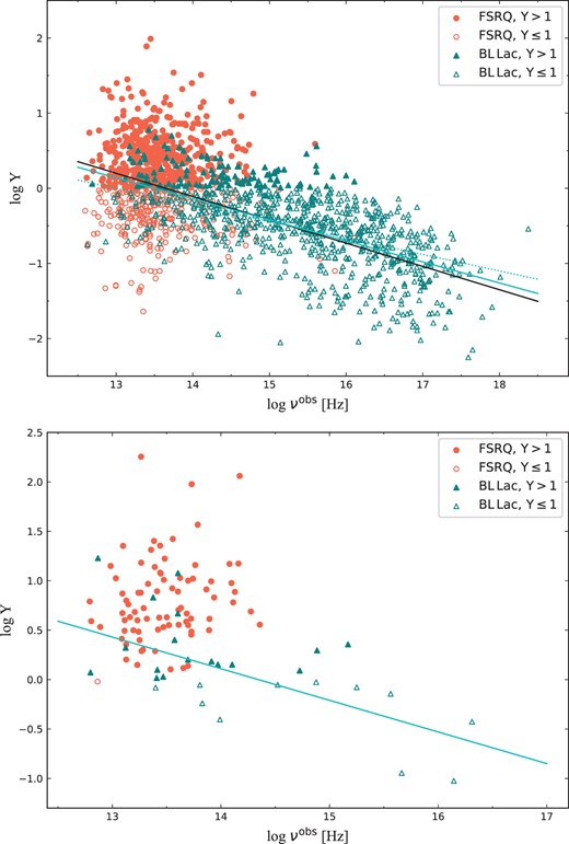
The correlations between log (Y) and log (ν^obs) in the historical sample (upper panel), and in the quasi-simultaneous sample (lower panel). As explained in the inset legends, the red symbol represents the FSRQs; the teal symbol represents the BL Lacs; the full symbol represents the source with Y > 1; and the empty symbol represents the source with Y ≤ 1. If a significant correlation is found (τ > 0.1, p < 0.01) for a specific (sub-) sample statistically, the best linear fitting equation is also shown. The solid black line represents the best-fitting equation for the whole sample. The solid red line represents the best-fitting equation for the whole population of FSRQs, the dashed red line represents the best-fitting equation for the population of FSRQs with Y > 1, and the dotted red line represents the best-fitting equation for the population of FSRQs with Y ≤ 1. The solid teal line represents the best-fitting equation for the whole population of BL Lacs; the dashed teal line represents the best-fitting equation for the population of BL Lacs with Y > 1; and the dotted teal line represents the best-fitting equation for the population of BL Lacs with Y ≤ 1.

Open in new tab Download slide

The correlations between |$\log (L^{\rm obs}_{\rm rad})$| and log (ν^obs) in the observers’ frame for the historical and quasi-simultaneous samples are shown in Fig. 2. A moderate negative correlation (τ = −0.48) is found in historical sample, which is consistent with many previous studies (Fossati et al. 1998; Chen & Bai 2011; Finke 2013; Xiong et al. 2015a; Fan et al. 2016b; Ghisellini et al. 2017), but no correlation (τ = −0.05) is found in quasi-simultaneous sample. When focusing on FSRQs, weak negative correlations are found both in historical (τ = −0.14) and quasi-simultaneous samples (τ = −0.2; also a large chance probability p = 0.08 is obtained for quasi-simultaneous sample). For BL Lacs in historical sample, no correlation is found for the whole sample and for subsample with Y ≤ 1. For BL Lacs with Y > 1, only a weak correlation with a large chance probability (τ = −0.17, p = 0.07) is found. For BL Lacs in quasi-simultaneous sample, weak correlations are found, but the chance probabilities are significant high (p > 0.3), suggesting that these correlations are not significant. Among the above results of the whole sample in the historical sample, our main focus is on the correlation between the full-band radiative luminosity and the peak frequency. In contrast, Yang et al. (2022a) focuses on the correlations between the peak frequency and radio, optical, X-ray, and γ-ray emissions, respectively. Given that most FSRQs have Y > 1, which means the γ-ray luminosity dominates the full-band radiative luminosity, our results are basically consistent with Yang et al. (2022a). However, for BL Lacs, the band that dominates the full-band radiative luminosity is uncertain. Therefore, it is difficult to directly compare our results with Yang et al. (2022a), which focuses on the correlation of a specific band. Our correlation study suggests that no correlation is found for the whole sample of BL Lacs. As can be seen from the upper panel of Fig. 2, no correlation found for the whole sample of BL Lacs may be due to the discovery of many high-luminosity HSPs and low-luminosity LSPs in the Fourth Fermi-LAT 12-yr Source catalogue. It is worth noting that our findings differ from those obtained using data from the third catalogue of AGN detected by Fermi-LAT (3LAC), where correlations are found in BL Lacs instead of FSRQs (Ghisellini et al. 2017). In addition, Fan et al. (2016b) find marginal correlations in BL Lacs-HSPs (τ = 0.1, p = 3.6 × 10⁻³) instead of FSRQs or BL Lacs-LSPs, and Mao et al. (2016) find strong correlations without particular separation between FSRQs and BL Lacs.

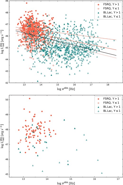
$The correlations between $\log (L_{\rm rad}^{\rm obs})$ and log (νobs) in the historical sample (upper panel), and in the quasi-simultaneous sample (lower panel). The meanings of symbols and line styles are the same as in Fig. 1. Similarly, the best linear fitting equation is only shown when a significant correlation is found.$

Figure 2.

The correlations between |$\log (L_{\rm rad}^{\rm obs})$| and log (ν^obs) in the historical sample (upper panel), and in the quasi-simultaneous sample (lower panel). The meanings of symbols and line styles are the same as in Fig. 1. Similarly, the best linear fitting equation is only shown when a significant correlation is found.

Open in new tab Download slide

Based on the results above, there are similarities and differences in correlation studies of the phenomenological blazar sequence between the historical and quasi-simultaneous samples. Some of these differences may be attributed to the fact that the quasi-simultaneous sample contains different states of SEDs (Xue et al. 2016), while others may be due to the small size of the quasi-simultaneous sample, resulting in p > 0.01. Moreover, for the quasi-simultaneous SED given by (Xue et al. 2016), the observation time for radio, optical, and X-ray is within one week, while the γ-ray data has been integrated over several months. However, variabilities on the scales of days (e.g. Bonning et al. 2012), hours (e.g. Hayashida et al. 2015), and even minutes (e.g. Begelman, Fabian & Rees 2008) have been widely observed in different energy bands of blazars. Therefore, using the quasi-simultaneous data collected by Xue et al. (2016) will introduce potential bias. It is interesting that if the correlation holds both for the historical and quasi-simultaneous samples, their s values are also quite close. In the subsequent theoretical interpretation (see Section 3), we choose to rely on the results of the historical sample. A larger quasi-simultaneous sample with high-quality and same state (high or low) SEDs is needed to check these results in detail.

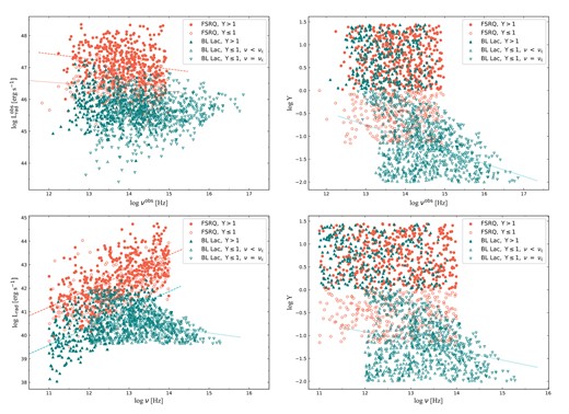
We study the intrinsic blazar sequence using the δ_D-corrected sample, and the correlation results are presented in Fig. 3. For the correlation between log (Y) and log (ν), weak correlations are found, but the obtained large chance probabilities (p > 0.1) suggesting that these correlations might not be significant. In contrast, a strong positive correlation (τ = 0.54) is found for the correlation between log (L_rad) and log (ν). Furthermore, when we study FSRQs and BL Lacs (dominated by ones with Y > 1), respectively, similar correlation results and slopes (s ∼ 1) are derived as well. The obtained positive correlations are consistent with those obtained by some previous works (Nieppola et al. 2008; Wu, Gu & Jiang 2009; Fan, Bai & Mao 2016a; Chen et al. 2021), and the obtained slopes are consistent with our previous studies (Fan et al. 2017; Yang et al. 2022b). It is noteworthy that δ_D used by Chen et al. (2021) are derived from the conventional one-zone leptonic model (Chen 2018). However, it is unfortunate that the slope of the best linear fitting equation is omitted in their study.

Figure 3.

The upper panel shows the correlations between log (L_rad) and log (ν), and the lower panel shows the correlations between log (Y) and log (ν) in the δ_D-corrected sample. The meanings of symbols and line styles are the same as in Fig. 1. Similarly, the best linear fitting equation is only shown when a significant correlation is found.

Open in new tab Download slide

3 THEORETICAL ANALYSIS

3.1 Simple scaling model

In the study of blazars, many phenomenological models have been proposed. However, most of these models contain numerous free parameters, even the simplest conventional one-zone model has at least seven free parameters that are coupled to each other. This may not be inappropriate for studying the global properties of blazars, such as the blazar sequence. In radio and X-ray observations, bright knots have been observed along the jet of blazars and radio galaxies (e.g. Marscher & Jorstad 2011; Mertens et al. 2016). In other words, significant dissipation regions can potentially appear at any location along the jet (Worrall et al. 2007; Ghisellini & Tavecchio 2009; Liu et al. 2023). This kind of framework that considers the dominant dissipation region appearing at different positions has been applied by Potter (2018) and Wang et al. (2022) to explain the orphan flares of blazars. Following this phenomenological framework, we assume that one single spherical dissipation region appearing at different position of the jet dominates the whole jet emission, which is certainly an oversimplified assumption (for a multizone view, please see Liu et al. 2023). This dominant dissipation region is composed of a plasma of charged particles in a uniform magnetic field B with radius R and moving with bulk Lorentz factor Γ = (1 − β²)^−1/2, where βc is the jet speed, along the jet, at a viewing angle θ^obs with respect to observers’ line of sight. By assuming θ^obs ≲ 1/Γ for blazars, we have δ_D ≈ Γ. Let us envision that the dominant dissipation regions of all blazars can be placed within one jet. In this way, these dominant dissipation regions are distributed at different positions within this jet. Based on some reasonable assumptions that usually applied in the continuous jet model (e.g. Blandford & Königl 1979), physical parameters of these dissipation regions are connected with each other. Radio observations have found that AGNs jets have an approximate conical (Kovalev et al. 2007; Sokolovsky et al. 2011) or parabolic structure (Nakamura & Asada 2013; Algaba et al. 2017; Giovannini et al. 2018; Hodgson et al. 2018). If assuming that the dissipation region occupies the entire jet cross-section, we have R∝r^α, where r is the distance between SMBH and the dissipation region. More specifically, α = 1 represents the jet has a conical structure, and 0 < α < 1 means the jet has a parabolic structure. For the magnetic field B, we have B∝R⁻¹∝r^−α by assuming the magnetic power is conserved in the jet (Blandford & Königl 1979), which is a crucial assumption for reproducing the flat radio spectrum (Potter & Cotter 2012). In addition, if considering the jet’s continuous acceleration or deceleration as suggested by phenomenological model, magnetohydrodynamic simulation, and observation (Blandford & Königl 1979; Hawley & Krolik 2006; Potter & Cotter 2013a; Mościbrodzka et al. 2014; Roychowdhury et al. 2024), we assume a simplified acceleration/deceleration profile, i.e. δ_D∝r^x, where x > 0 for an accelerating jet, x < 0 for a decelerating jet, and x = 0 for a constant-speed jet or δ_D does not related to other parameters. In this way, power-law scaling connections of R, B, δ_D, and r can be established. With this simple scaling model, the potential physical origins of the statistical correlation of the blazar sequence can be investigated. Of course, one should bear in mind that the jet each dissipation region located in is actually different; therefore; the normalization of each power-law correlations is still a free parameter. In this section, parameters with superscript ‘obs’ are measured in observers’ frame, whereas the parameters without the superscript are measured in the comoving frame, unless specified otherwise.

Assuming that accelerated relativistic electrons are injected in the dissipation region with a specific spectral shape Ω(γ) at a constant rate given by |$\dot{Q}(\gamma)=\dot{Q}_0\Omega (\gamma), \gamma _{\rm min}\lt \gamma \lt \gamma _{\rm max},$| where γ_min is the minimum electron Lorentz factor, γ_max is the maximum electron Lorentz factor, and |$\dot{Q}_0$| is the normalization in units of |$\rm cm^{-3}~s^{-1}$|⁠. By giving an electron injection luminosity L_inj, |$\dot{Q}_0$| can be calculated by

$$\begin{eqnarray} \dot{Q}_0=\frac{L_{\rm inj}}{V_{\rm b}mc^2\int _{\gamma _{\rm min}}^{\gamma _{\rm max}} \gamma \Omega (\gamma)d\gamma }, \end{eqnarray}$$

(1)

where m is the rest mass of an electron, c is the speed of light, and V_b is the volume of the dissipation region. The radiative luminosity (i.e. the bolometric luminosity) in the comoving frame can be calculated as

$$\begin{eqnarray} L_{\rm rad}=V_{\rm b}mc^2\int _{\gamma _{\rm min}}^{\gamma _{\rm max}} f(\gamma)\gamma \dot{Q}(\gamma){\rm d}\gamma , \end{eqnarray}$$

(2)

where |$f(\gamma)=\rm min\lbrace \frac{{\it t}_{\rm dyn}}{{\it t}_{\rm cool}}, 1\rbrace$| is the cooling efficiency of electrons. More specifically, t_dyn = ηR/c with η > 1 is the dynamical time-scale² and t_cool = 3mc/[4γσ_TU_B(1 + Y)] is the radiative cooling time-scale, where σ_T is the Thomson scattering cross-section, U_B = B²/(8π) is the energy density of the magnetic field, and Y is the Compton dominance. In this work, we aim to study if radiative cooling is responsible for the blazar sequence, so it is more appropriate to use the full-band radiative luminosity L_rad.

Substituting equation (1) into equation (2), we have

$$\begin{eqnarray} L_{\rm rad}&=&\frac{L_{\rm inj}}{\int _{\gamma _{\rm min}}^{\gamma _{\rm max}} \gamma \Omega (\gamma){\rm d}\gamma }\int _{\gamma _{\rm min}}^{\gamma _{\rm max}}f(\gamma)\gamma \Omega (\gamma){\rm d}\gamma \\ &=&\frac{L_{\rm inj}}{\int _{\gamma _{\rm min}}^{\gamma _{\rm max}} \gamma \Omega (\gamma){\rm d}\gamma } \bigg \lbrace \int _{\gamma _{\rm c}}^{\gamma _{\rm max}} \gamma \Omega (\gamma){\rm d}\gamma + \frac{f(\gamma)}{\gamma }\int _{\gamma _{\rm min}}^{\gamma _{\rm c}}\gamma ^2 \Omega (\gamma){\rm d}\gamma \bigg \rbrace \\ &&\propto L_{\rm inj}(\gamma \gt \gamma _{\rm c})+L_{\rm inj}(\gamma \lt \gamma _{\rm c})B^2R(1+Y),\\ \end{eqnarray}$$

(3)

where |$\gamma _{\rm c}=\frac{3mc^2}{4\sigma _{\rm T}RU_{\rm B}(1+Y)}$| represents the cooling break at which t_dyn = t_cool.

Following the physical interpretation of Ghisellini et al. (1998), if we believe that the peak of the low-energy component is caused by radiative cooling, the peak frequency in the comoving frame can be estimated using the monochromatic approximation (Tavecchio, Maraschi & Ghisellini 1998)

$$\begin{eqnarray} \nu &\approx 3.7\times 10^6 \gamma _{\rm c}^2B \\ &\propto B^{-3}R^{-2}(1+Y)^{-2}. \end{eqnarray}$$

(4)

From equations (3) and (4), it can be seen that expressions of L_rad, ν, and Y (its expression will be given later) consist of several physical parameters coupled together, including R, B, and δ_D. Considering connections of R, B, δ_D, and r in the framework of the simple scaling model, L_rad becomes

$$\begin{eqnarray} L_{\rm rad} \propto L_{\rm inj}(\gamma \gt \gamma _{\rm c})+L_{\rm inj}(\gamma \lt \gamma _{\rm c})(1+Y)r^{-\alpha }, \end{eqnarray}$$

(5)

and ν becomes

$$\begin{eqnarray} \nu \propto r^{\alpha }(1+Y)^{-2}. \end{eqnarray}$$

(6)

For FSRQs, the Compton dominance Y can be evaluated as

$$\begin{eqnarray} Y&\simeq \frac{\delta _{\rm D}^2U_{\rm ext}}{U_{\rm B}} \\ &\propto \left\lbrace \begin{array}{rl}r^{2\alpha +2x}, r\lt r_{\rm ext} \\ r^{2\alpha +2x-n}, r\gt r_{\rm ext} \end{array} \right., \end{eqnarray}$$

(7)

where U_ext is the energy density of the external photon field in the AGN frame, and r_ext represents the characteristic distance of external photon fields that is found to scale with the disc luminosity L_D as r_ext∝L_D^1/2 through reverberation mapping (Suganuma et al. 2006; Kishimoto et al. 2011; Bentz et al. 2013; Pozo Nuñez et al. 2014). When the dissipation region is located within r_ext, |$U_{\rm ext}=L_{\rm D}/(4\pi r_{\rm ext}^2c)$| would be a constant value (Harvey, Georganopoulos & Meyer 2020); when the dissipation region is located beyond r_ext, U_ext decreases with the index n (Sikora et al. 2009; Hayashida et al. 2012). From equations (6) and (7), the non-linear correlation between the synchrotron peak frequency and the Compton dominance in logarithmic space can be obtained

$$\begin{eqnarray} \nu \propto \left\lbrace \begin{array}{rl}Y^{\frac{\alpha }{2\alpha +2x}}(1+Y)^{-2}, r\lt r_{\rm ext} \\ Y^{\frac{\alpha }{2\alpha +2x-n}}(1+Y)^{-2}, r\gt r_{\rm ext} \\ \end{array} \right. \end{eqnarray}$$

(8)

in the comoving frame, and

$$\begin{eqnarray} \nu ^{\rm obs} \propto \left\lbrace \begin{array}{rl}Y^{\frac{1}{2}}(1+Y)^{-2}, r\lt r_{\rm ext} \\ Y^{\frac{\alpha +x}{2\alpha +2x-n}}(1+Y)^{-2}, r\gt r_{\rm ext} \\ \end{array} \right. \end{eqnarray}$$

(9)

in the observers’ frame. If considering Y ≪ 1 and Y ≫ 1,³ above correlations become linear in logarithmic space, i.e.

$$\begin{eqnarray} Y\propto \left\lbrace \begin{array}{rl}\nu ^{\frac{2\alpha +2x}{\alpha }}, r\lt r_{\rm ext} \\ {\nu }^{\frac{2\alpha +2x-n}{\alpha }}, r\gt r_{\rm ext} \end{array} \right., Y\ll 1\\ Y\propto \left\lbrace \begin{array}{rl}\nu ^{\frac{2\alpha +2x}{-3\alpha -4x}}, r\lt r_{\rm ext} \\ {\nu }^{\frac{2\alpha +2x-n}{2n-3\alpha -4x}}, r\gt r_{\rm ext} \end{array} \right., Y\gg 1 \end{eqnarray}$$

(10)

in the comoving frame, and

$$\begin{eqnarray} Y\propto \left\lbrace \begin{array}{rl}{\nu ^{\rm obs}}^2, r\lt r_{\rm ext} \\ {\nu ^{\rm obs}}^{\frac{2\alpha +2x-n}{\alpha +x}}, r\gt r_{\rm ext} \end{array} \right., Y\ll 1\\ Y\propto \left\lbrace \begin{array}{rl}{\nu ^{\rm obs}}^{-2/3}, r\lt r_{\rm ext} \\ {\nu ^{\rm obs}}^{\frac{2\alpha +2x-n}{2n-3\alpha -3x}}, r\gt r_{\rm ext} \end{array} \right., Y\gg 1 \end{eqnarray}$$

(11)

in the observers’ frame. It should be noted that due to the actual correlation being non-linear, when Y ∼ 1, under certain combinations of α, n, and x, the true slope may have significant errors compared to those when Y ≪ 1 and Y ≫ 1. From equation (5), it can be seen that if the first term on the right is dominant, the correlation between ν and L_rad depends on if there is a correlation between ν and L_inj. Assuming that the first term on the right is not dominant and values of L_inj do not have a large dispersion, we have

$$\begin{eqnarray} L_{\rm rad}\propto \left\lbrace \begin{array}{rl}&{\nu }^{-1}, {\it Y}\ll 1 \\ &{\nu }^{\frac{2x+\alpha }{-3\alpha -4x}}, {\it Y}\gg 1, r\lt r_{\rm ext} \\ &{\nu }^{\frac{2x+\alpha -n}{2n-3\alpha -4x}}, {\it Y}\gg 1, r\gt r_{\rm ext} \end{array} \right. \end{eqnarray}$$

(12)

in the comoving frame, and

$$\begin{eqnarray} L_{\rm rad}^{\rm obs}\propto \left\lbrace \begin{array}{rl}&{\nu ^{\rm obs}}^{\frac{4x-\alpha }{x+\alpha }}, {\it Y}\ll 1 \\ &{\nu ^{\rm obs}}^{\frac{6x+\alpha }{-3\alpha -3x}}, {\it Y}\gg 1, r\lt r_{\rm ext} \\ &{\nu ^{\rm obs}}^{\frac{6x+\alpha -n}{2n-3\alpha -3x}}, {\it Y}\gg 1, r\gt r_{\rm ext} \end{array} \right. \end{eqnarray}$$

(13)

in the observers’ frame. Note that the above analysis is based on the assumption that radiative cooling induces the spectrum break. However, cooling induced change of spectral index is rarely discovered in observations (Baheeja et al. 2022). Therefore, it is necessary to re-study these two correlations for ν < ν_c. In this scenario, electrons are cooled in slow cooling regime, so the break of the electron energy distribution corresponding to the peak frequency of the low-energy component might be ascribed to multiple acceleration processes (Bell 1978b; Tan, Liu & Böttcher 2023). In the diffusive shock acceleration, the electron Lorentz factor can be evaluated as γ ∝ BR (Axford, Leer & Skadron 1977; Blandford & Ostriker 1978; Bell 1978a, b; Kirk & Schneider 1988; Rieger, Bosch-Ramon & Duffy 2007), therefore ν∝B³r²∝r^−α. Then, for the correlation between the synchrotron peak frequency and the Compton dominance, we have

$$\begin{eqnarray} Y\propto \left\lbrace \begin{array}{rl}\nu ^{-\frac{2\alpha +2x}{\alpha }}, r\lt r_{\rm ext} \\ {\nu }^{-\frac{2\alpha +2x-n}{\alpha }}, r\gt r_{\rm ext} \end{array} \right. \end{eqnarray}$$

(14)

in the comoving frame, and

$$\begin{eqnarray} Y\propto \left\lbrace \begin{array}{rl} {\nu ^{\rm obs}}^{\frac{2\alpha +2x}{x-\alpha }}, r\lt r_{\rm ext}\\ {\nu ^{\rm obs}}^{\frac{2\alpha +2x-n}{x-\alpha }}, r\gt r_{\rm ext} \end{array} \right. \end{eqnarray}$$

(15)

in the observers’ frame. For the correlation between the synchrotron peak frequency and the radiative luminosity, we have

$$\begin{eqnarray} L_{\rm rad}\propto \left\lbrace \begin{array}{rl}&\nu , {\it Y}\ll 1 \\ &{\nu }^{-\frac{2x+\alpha }{\alpha }}, {\it Y}\gg 1, r\lt r_{\rm ext} \\ &{\nu }^{-\frac{2x+\alpha -n}{\alpha }}, {\it Y}\gg 1, r\gt r_{\rm ext} \end{array} \right. \end{eqnarray}$$

(16)

in the comoving frame, and

$$\begin{eqnarray} L_{\rm rad}^{\rm obs}\propto \left\lbrace \begin{array}{rl}&{\nu ^{\rm obs}}^{\frac{4x-\alpha }{x-\alpha }}, {\it Y}\ll 1 \\ &{\nu ^{\rm obs}}^{\frac{6x+\alpha }{x-\alpha }}, {\it Y}\gg 1, r\lt r_{\rm ext} \\ &{\nu ^{\rm obs}}^{\frac{6x+\alpha -n}{x-\alpha }}, {\it Y}\gg 1, r\gt r_{\rm ext} \end{array} \right. \end{eqnarray}$$

(17)

in the observers’ frame.

For BL Lacs, the Compton dominance Y can be evaluated as

$$\begin{eqnarray} Y\simeq \frac{U_{\rm syn}}{U_B}, \end{eqnarray}$$

(18)

where |$U_{\rm syn}=L_{\rm rad}^{\rm syn}/(4\pi R^2c)$| is the energy density of synchrotron photons, |$L_{\rm rad}^{\rm syn}$| represents the radiative synchrotron luminosity

$$\begin{eqnarray} L_{\rm rad}^{\rm syn}=V_{\rm b}mc^2\int _{\gamma _{\rm min}}^{\gamma _{\rm max}} f_{\rm syn}(\gamma)\gamma \dot{Q}(\gamma){\rm d}\gamma , \end{eqnarray}$$

(19)

where |$f_{\rm syn}(\gamma)=\rm min\lbrace \frac{{\it t}_{\rm dyn}}{{\it t}_{\rm syn}}, 1\rbrace$| is the cooling efficiency of synchrotron emission. Then Y can be written as

$$\begin{eqnarray} Y\propto L_{\rm inj}(\gamma \gt \gamma _{\rm c})+L_{\rm inj}(\gamma \lt \gamma _{\rm c})r^{-\alpha }. \end{eqnarray}$$

(20)

First, we study the correlations of the blazar sequence for ν = ν_c. If Y’s the first term on the right is dominant, the correlation between ν and Y depends on if there is a correlation between ν and L_inj. If the first term on the right is not dominant, we derive the correlation between ν and Y,

$$\begin{eqnarray} Y\propto \left\lbrace \begin{array}{rl}&{\nu }^{-1}, Y\ll 1 \\ &{\nu }^{-\frac{1}{3}}, {\it Y}\gg 1 \end{array} \right. \end{eqnarray}$$

(21)

in the comoving frame, and

$$\begin{eqnarray} Y\propto \left\lbrace \begin{array}{rl}&{\nu ^{\rm obs}}^{-\frac{\alpha }{\alpha +x}}, Y\ll 1 \\ &{\nu ^{\rm obs}}^{-\frac{\alpha }{3\alpha +x}}, {\it Y}\gg 1 \end{array} \right. \end{eqnarray}$$

(22)

in the observers’ frame. Similarly, we derive the correlation between the synchrotron peak frequency and the radiative luminosity, i.e.

$$\begin{eqnarray} L_{\rm rad}\propto \left\lbrace \begin{array}{rl}&{\nu }^{-1}, {\it Y}\ll 1 \\ &{\nu }^{-2/3}, {\it Y}\gg 1 \end{array} \right. \end{eqnarray}$$

(23)

in the comoving frame, and

(24)

in the observers’ frame.

Similar to previous discussion for FSRQs, we also study these two correlations for BL Lacs in the case of ν < ν_c, i.e. ν∝B³r²∝r^−α. For the correlation between the synchrotron peak frequency and the Compton dominance (equation 20), we have

$$\begin{eqnarray} Y\propto {\nu } \end{eqnarray}$$

(25)

in the comoving frame, and

$$\begin{eqnarray} Y\propto {\nu ^{\rm obs}}^{\frac{\alpha }{\alpha -x}} \end{eqnarray}$$

(26)

in the observers’ frame. For the correlation between the synchrotron peak frequency and the radiative luminosity, we have

$$\begin{eqnarray} L_{\rm rad}\propto \left\lbrace \begin{array}{rl}&\nu , {\it Y}\ll 1 \\ &\nu ^{2}, {\it Y}\gg 1 \end{array} \right. \end{eqnarray}$$

(27)

in the comoving frame, and

$$\begin{eqnarray} L_{\rm rad}^{\rm obs}\propto \left\lbrace \begin{array}{rl}&{\nu ^{\rm obs}}^{\frac{4x-\alpha }{x-\alpha }}, {\it Y}\ll 1 \\ &{\nu ^{\rm obs}}^{\frac{4x-2\alpha }{x-\alpha }}, {\it Y}\gg 1 \end{array} \right. \end{eqnarray}$$

(28)

in the observers’ frame.

As deduced above, we obtain equations of the blazar sequence for FSRQs and for BL Lacs in the comoving and observers’ frames, respectively. All equations are summarized in Table 2. By taking the logarithm of the parameters in the correlations, we can get the corresponding slopes, which can be compared with the statistical linear regression results.

Table 2.

Open in new tab

Deduced equations of the correlations in the blazar sequence.

The simple scaling model proposed in this subsection is quite similar to the conventional one-zone model, where all the jet emission is represented by one single dissipation region. Compared to the conventional one-zone model, the advantage of this simple scaling model is that power-law relationships have been established among several physical parameters based on reasonable assumptions. However, normalizations of power-law relationships for each blazar remains unknown and varies. This will greatly increase the dispersion of the correlation intercept, even if the correlation slope predicted by the model is the same. Moreover, the simple scaling model, compared to the conventional one-zone model, takes many shortcuts. For example, to establish the power-law correlations among multiple physical parameters, a crude assumption is introduced, i.e. the electron injected luminosities of all blazars do not have a large dispersion. However, as suggested by Ghisellini & Tavecchio (2008), the black hole mass and the accretion rate would be crucial for interpreting the blazar sequence, since the jet power is always linked with the accretion rate. Therefore, such an assumption is likely to generate potential bias. Also, blazars have a complex environment with various external photon fields, such as the BLR, the DT, etc., each with its own unique influence distance. Gathering information on each blazar’s external photon field is tough, so we make an simplification that there is just one main external photon field. When using the conventional one-zone model to interpret blazars’ SEDs, the evolution of the relativistic electron energy distribution is a factor that cannot be ignored. However, in our attempt to understand the blazar sequence using the simple scaling model, we do not specify the particular shape for the electron energy distribution, nor do we study its evolution. This simplification is feasible because the study of the blazar sequence only requires information about the synchrotron peak frequency and integrated luminosity, both of which can be obtained through analytical calculations.

3.2 Theoretical implications

In this subsection, we apply the simple scaling model described in Section 3.1 to interpret the statistical correlation results of the phenomenological and intrinsic blazar sequence derived in Section 2.

First of all, let us investigate if statistical results can be interpreted under the conditions that ν = ν_c, i.e. cooling is important. As mentioned before, values of δ_D given by radio observation may have a great discrepancy with the actual values of δ_D. If one consider that radio δ_D is significantly influential and unreliable, or if we believe that the distribution of actual δ_D is irregular, i.e. x = 0, then it can be seen from Table 2 that the synchrotron peak frequency is both anticorrelated with the Compton dominance and the radiative luminosity in the observers’ and comoving frames. This is consistent with the original physical interpretation proposed by Ghisellini et al. (1998). If here we trust the radio δ_D and believe in the correlation results of the intrinsic blazar sequence, then the physical explanation of cooling might faces difficulties. From the statistical results in Table 1, it can be seen that no correlation is found between the Compton dominance and the synchrotron peak frequency for all (sub-)samples of FSRQs, whether in the observers’ frame or the comoving frame. It indicates that indexes of the deduced equations (10) and (11) are zero, i.e. r > r_ext and 2α + 2x − n = 0. Consequently, the indexes of equation (12) between L_rad and ν in the comoving frame become −1. In addition, equation (23) suggests that L_rad is negatively correlated with ν for BL Lacs in the comoving frame (even when considering the actual non-linear correlation). However, moderate and strong positive correlations between L_rad and ν are found for FSRQs and BL Lacs, respectively, implying a different physical origin of these correlations. In the following, we will discuss if deduced equations under the condition that ν < ν_c have the potential to account for the phenomenological and intrinsic blazar sequence simultaneously.

For FSRQs, if we consider r < r_ext, equations (14) and (15) suggest that x should be equal to −α, since no correlation is found between the Compton dominance and the synchrotron peak frequency both in the observers’ frame and the comoving frame. Consequently, the index of equation (16) becomes unity (including the case Y ≪ 1), which is consistent with the statistical results. However, the index of equation (17) will be 5/2, which is inconsistent with the statistical results that found s = −0.35 when Y ≤ 1 and s = −0.18 when Y > 1. Therefore, we need to further discuss the case of r > r_ext. In this case, since statistical studies find that the Compton dominance and the synchrotron peak frequency are not correlated, equations (14) and (15) suggest that 2α + 2x − n = 0. Moreover, by making the indexes of equations (16) and (17) equal to the slopes obtained in the statistical studies (including errors), we can get combinations of x, n, and α that satisfies all conditions, which are shown in Fig. 4. It can be seen that the size of effective intersection area is proportional to the value of α. It implies that the effective parameter space can only be obtained when x > 0, i.e. the dissipation region has to be located in the accelerating jet. We emphasize that any combinations of x, n, and α that satisfies 2α + 2x − n = 0 are possible. In Fig. 4, we present five sets of parameter combinations, which are α = 1, n ≃ 2.6, x ≃ 0.3; α = 0.8, n ≃ 2.1, x ≃ 0.24; α = 0.6, n ≃ 1.56, x ≃ 0.18; α = 0.4, n ≃ 1.04, x ≃ 0.12; and α = 0.2, n ≃ 0.52, x ≃ 0.06. Please note that our discussion here is based on the assumption of a single external photon field, which is a simplification. In the actual AGNs’ environment, it is generally believed that there are two external photon fields, i.e. the BLR and the DT, both of which could have significant implications for jet emission. For the BLR, n = 3 has been suggested as a model assumption by Sikora et al. (2009). For the DT, n = 4 has been found by Hayashida et al. (2012) for a specific observation of an FSRQ 3C 279. While it may not be the case that n = 3 or n = 4 works for every AGN, our results clearly suggest that the majority of AGNs cannot have an n greater than 3. Otherwise, α would be larger than 1, implying that the jet profile becomes hyperbolic. This is evidently in contradiction with the conical or parabolic structure found by radio observations (see Blandford, Meier & Readhead 2019, for a review). On the other hand, the covering factors, which represent the fractions of the disc luminosity reprocessed into the BLR and DT radiation, evidently vary among different AGNs. For instance, values such as 0.1, 0.2, and 0.5 have been suggested (Maiolino et al. 2007; Ghisellini & Tavecchio 2009; Hao et al. 2010, 2011). This degree of variability introduces complexity into the model interpretation attempted here, and may even preclude the possibility of reaching definitive conclusions. Therefore, the assumption of a single external photon field in this work is a simplifying approximation. In general, our model suggests that the phenomenological and intrinsic blazar sequence of FSRQs can be explained only when the condition 2α + 2x − n = 0 is satisfied, implying that the dissipation region is in an accelerating jet located beyond the external photon field in the slow-cooling regime.

Figure 4.

Parameter spaces for FSRQs with different value of α when r > r_ext. Solid curves represent that the indexes of equations (14) and (15) are equal to zero, as statistical analysis find that Y and ν (or ν^obs) are not correlated. Dashed, dotted, and dash–dotted curves are obtained by setting the indexes of equations (16) and (17) equal to slopes obtained from statistical analysis, respectively. Since errors of slopes are also taken into account, the intersection area between two curves of each type represents the effective parameter space. After considering the intersection of all line types, we find the corresponding combinations of n, x, and α, which are marked by red circles.

Open in new tab Download slide

For BL Lacs, the physical interpretation of phenomenological and intrinsic blazar sequence appears to be complicated. For BL Lacs with Y > 1, the derived correlation results and slopes (if correlations exist) are similar to those of FSRQs. On the other hand, we find that BL Lacs with Y > 1 in different samples are dominated by LSPs (61/118 = 52 per cent for historical sample, 14/17 = 82 per cent for quasi-simultaneous sample, and 23/51 = 45 per cent for δ_D-corrected sample), which may suggest that their high-energy components are mainly from the EC emission rather than the SSC emission (Böttcher 2007; Böttcher et al. 2013; Wang & Xue 2021; Deng & Jiang 2023). Blazars are classified as FSRQs and BL Lacs based on whether broad emission lines are detected. However, there are many blazars with comparable jet and broad emission lines intensities that are classified into either subclass depending on the jet activity during observation. For instance, if the jet emission is in a low state during observation, the blazar will be observed with broad emission lines and classified as FSRQs. On the other hand, if the jet emission is in a high state, the emission lines will be masked, then the blazar will be classified as BL Lacs. Such blazars are known as ‘changing-look’ blazars (Matt, Guainazzi & Maiolino 2003; Bianchi et al. 2005). Additionally, some blazars with broad emission lines are classified as BL Lacs because their broad emission lines are outshone by the jet emission. These blazars are suggested as ‘masquerading’ BL Lacs (Giommi, Padovani & Polenta 2013). In our sample, eighteen blazars (including 4FGL J0238.6 + 1637, 4FGL J0334.2 − 4008, 4FGL J0407.5 + 0741, 4FGL J0428.6 − 3756, 4FGL J0438.9 − 4521, 4FGL J0516.7 − 6207, 4FGL J0538.8 − 4405, 4FGL J0629.3 − 1959, 4FGL J0710.9 + 4733, 4FGL J0831.8 + 0429, J1001.1 + 2911, 4FGL J1058.4 + 0133, 4FGL J1147.0 − 3812, 4FGL J1751.5 + 0938, 4FGL J1800.6 + 7828, 4FGL J1954.6 − 1122, 4FGL J2134.2 − 0154, and 4FGL J2152.5 + 1737) are suggested as changing-look blazars (Xiao et al. 2022), which can be seen as the direct evidence of presence of external photon fields. Our recent work also suggests that BL-LSPs are masquerading BL Lacs (Hu et al.2024). Therefore, we suggest that the phenomenological and intrinsic blazar sequence of BL Lacs with Y > 1 can also be explained by the dissipation region in accelerating jet (located beyond the external photon field) emitting in the slow-cooling regime, as in FSRQs. For BL Lacs with Y ≤ 1, we do not find enough BL Lacs with measured δ_D in the literature, so we only study the phenomenological blazar sequence. For the phenomenological correlations, no correlation is found between |$\log (L_{{\rm rad}}^{{\rm obs}})~ {\rm vs.}~ \log (\nu ^{{\rm {obs}}})$|⁠, indicating the indexes of equation (24, 28) are zeros, i.e. 4x − α = 0. Since 0 < α ≤ 1, it indicates that the dissipation region is in an accelerating jet with 0 < x ≤ 0.25 (no matter ν = ν_c or ν < ν_c). If defaulting x = 0.25, the obtained strong negative correlation between log (Y) and log (ν^obs) can be explained in the case of ν = ν_c. Such a cooling scenario is quite possible for BL Lacs with Y ≤ 1, since HSPs are dominant in the historical (472/726 = 65 per cent) and quasi-simultaneous (5/11 = 45 per cent) samples. On the other hand, it is necessary to note that the model predicted slope (−0.8) for the correlation between log (Y) and log (ν^obs) is lower than that derived by the statistical analysis (∼−0.2). We suppose that this might be due to the BL Lacs in two samples having mixed cooling regimes, since the model predicted correlations under two cooling scenarios are opposite as shown in Table 2. Here, we emphasize that the above discussion assumes x = 0.25 merely for the convenience of showing that the statistical correlations could be reproduced based on some specific conditions. In fact, any combination of x and α that satisfies 4x − α = 0 is plausible. Furthermore, the attempt of introducing mixed cooling scenarios arises from the single cooling scenario’s inadequacy to account for the slope derived from statistical analysis.

3.3 Reproducing the blazar sequence

In previous, our theoretical analysis of the blazar sequence focuses on the power-law relation between various parameters (summarized in Table 2), as the obtained indexes can be compared with slopes given by correlation studies. However, specific values of normalization in power-law relations are ignored, which will inevitably increase the dispersion of the correlation. In addition, we do not provide specific values for each physical parameter, so one may worry that special and unreasonable physical parameters will be introduced. On the other hand, as shown in Section 3.1, the two correlations of the blazar sequence under some conditions are non-linear, which will have a certain impact on the slope and dispersion of the correlation. In this subsection, we would like to apply the simple scaling model to reproduce the blazar sequence shown in Figs 1–3, and provide the distribution of important physical parameters. In the following, we default that the jet has a conical structure (i.e. α = 1) as the benchmark case, as found in observations (Kovalev et al. 2007; Sokolovsky et al. 2011) and assumed in theoretical models (Kaiser 2006; Potter & Cotter 2012).

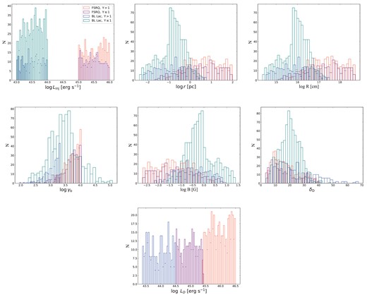
Applying the simple scaling model, 1800 blazars, including 300 FSRQs with Y ≤ 1, 500 FSRQs with Y > 1, 700 BL Lacs with Y ≤ 1 and 300 BL Lacs with Y > 1, are generated that are similar in composition to the historical sample. The physical parameters of these FSRQs and BL Lacs are assigned by generating random numbers from a certain range of values, following either a normal or uniform distribution. It is expected that model generated slopes are consistent with those in Table 1, so we assume that values of n and x of FSRQ and BL Lacs with Y > 1, respectively, conform to normal distributions with a mean of 2.6 and a standard deviation of 0.1, and a mean of 0.3 and a standard deviation of 0.05. For BL Lacs with Y < 1, values of x conform to a normal distribution with a mean of 2.5 and a standard deviation of 0.1. Values of the other physical parameters conform to uniform distributions within physically plausible ranges. For all blazars, uniform distributions of some parameters have the same range: 0.1^○ ≤ θ_open ≤ 3^○ (θ_open represents the jet half opening angle; Finke 2019); |$r_{\rm ext} \leqslant {\it r} \leqslant \rm 10^{2}~ pc$|⁠; 1 ≤ η ≤ 10 (Inoue & Takahara 1996; Mücke & Protheroe 2001; Gao, Pohl & Winter 2017); 1 ≤ δ_D,0 ≤ 3 (δ_D,0 represents the initial δ_D); and 2 ≤ s_e ≤ 4⁴ (s_e represents the spectral index of electrons energy distribution). In addition, there are some differences in the range of uniform distributions of L_inj, B, and L_D. For FSRQs, we set |$10^{45}~\rm erg~s^{-1} \leqslant {\it L}_{\rm inj} \leqslant \rm 10^{46}~erg~s^{-1}$|⁠; |$0.1~\rm G \leqslant {\it B}_{\rm 1pc} \leqslant \rm 1~G$| (B_1pc represents the magnetic field at 1 pc); and |$10^{44.5}~\rm erg~s^{-1} \leqslant {\it L}_{\rm D} \leqslant \rm 10^{46.5}~erg~s^{-1}$|⁠. For BL Lacs with Y > 1, we set |$10^{43}~\rm erg~s^{-1} \leqslant {\it L}_{\rm inj} \leqslant \rm 10^{44}~erg~s^{-1}$|⁠; |$0.01~\rm G \leqslant {\it B}_{\rm 1pc} \leqslant \rm 0.1~G$|⁠; and |$10^{42.5}~\rm erg~s^{-1} \leqslant {\it L}_{\rm D} \leqslant \rm 10^{44.5}~erg~s^{-1}$|⁠. For BL Lacs with Y < 1, we set |$10^{43}~\rm erg~s^{-1} \leqslant {\it L}_{\rm inj} \leqslant \rm 10^{44}~erg~s^{-1}$| and |$0.05~\rm G \leqslant {\it B}_{\rm 1pc} \leqslant \rm 0.5~G$|⁠. Based on the chosen ranges and distributions of parameters described above, the phenomenological and intrinsic blazar sequence generated by the simple scaling model are shown in Fig. 5, and the corresponding correlation results are given in Table 3. It can be seen that although the model generated correlation results and slopes are basically consistent with those of historical sample and δ_D-corrected sample, there are morphological differences between the data distribution obtained from the model and the observed data when viewed with the naked eye. For the correlation results, one major difference is that the slope of the correlation between |$\log (L_{{\rm rad}}^{{\rm obs}})$| and log (ν^obs) for FSRQs with Y ≤ 1 generated by the model is −0.10 ± 0.04, while the slope obtained from the historical sample is −0.35 ± 0.08. This may be due to the fact that the EC emission of these FSRQs with Y ≤ 1 no longer dominates the high-energy peak, which has changed the slope to some extent. On the other hand, our model, under the current settings, gives the predicted correlation results of FSRQs and BL Lacs with Y ≤ 1, respectively, which can be checked in the future with larger and more complete samples. Distributions of physical parameters are shown in Fig. 6. It can be seen that parameters distributions are generally reasonable and consistent with those suggested in the conventional leptonic model (Chen 2018; Cerruti 2020; Tan et al. 2020). However, it should be noted that the parameters distributions obtained here are only used to show that the phenomenological and intrinsic blazar sequence can be reproduced by the simple scaling model within a reasonable parameter range, and may not necessarily represent the actual physical properties of blazars. In fact, the blazar sequence currently reproduced using this simple scaling model may not necessarily have universal applicability. Although power-law correlations are built between physical parameters with reasonable assumptions, the normalizations are all random numbers, which greatly increases the dispersion and weakens the correlation. For example, as shown in Table 3, except for log (L_rad) versus log (ν), all others are weakly correlated or uncorrelated. If the range of parameter distributions continues to expand, e.g. L_inj, all the relevant correlations will disappear or the slope will change largely. Actually, Ghisellini & Tavecchio (2008) suggest that the accretion rate, which is directly related to L_inj, is important for the explanation of the blazar sequence. Therefore, the model generated results are highly sensitive to the chosen ranges and distributions of parameters. Further study is needed to identify the parameters that truly dominate. In addition, the actual blazar radiation mechanism must be more complex than the model we currently used. For example, the AGN environment contains multiple external photon fields, rather than the current single external photon field assumption; the jet acceleration profile is more complex and not even continuous; observations indicate that some jets have a parabolic structure (Nakamura & Asada 2013; Algaba et al. 2017; Giovannini et al. 2018). As a result, correlations of the historical sample are mostly weakly correlated or uncorrelated as well, and the correlation obtained from different samples also varies, as discussed in Section 2.2.

Figure 5.

The phenomenological (upper two panels) and intrinsic (lower two panels) blazar sequence generated by the simple scaling model. Similar to Figs 1–3, if a significant correlation is found (τ > 0.1, p < 0.01) for a specific subsample statistically, the best linear fitting equation is also shown. Red and teal dashed lines represent the best-fitting equation for the populations of FSRQs and BL Lacs with Y > 1, respectively. Red and teal dotted lines represent the best-fitting equation for the populations of FSRQs and BL Lacs with Y ≤ 1, respectively. The meanings of symbols are explained in the inset legends.

Open in new tab Download slide

$Distributions of the electron injection luminosity log Linj, the distance between SMBH and the dissipation region log r, the radius of the dissipation region log R, the electron Lorentz factor corresponding to the synchrotron peak frequency log γb, the magnetic field in the dissipation region log B, the Doppler factor of the dissipation region log δD, and the disc luminosity log LD. Mean values for FSRQs are, $\bar{L}_{\rm inj}=3.2\times 10^{45}\rm ~erg~s^{-1}$, $\bar{r}=3.5~\rm pc$, $\bar{R}=1.9\times 10^{17}\rm ~cm$, $\bar{\gamma }_{\rm b}=4.8\times 10^3$, $\bar{B}=0.3\rm ~G$, $\bar{\delta }_{\rm D}=16.8$, $\bar{L}_{\rm D}=3.6\times 10^{45}\rm ~erg~s^{-1}$, respectively. Mean values for BL Lacs are $\bar{L}_{\rm inj}=3.3\times 10^{43}\rm ~erg~s^{-1}$, $\bar{r}=0.14\rm ~pc$, $\bar{R}=7.8\times 10^{15}\rm ~cm$, $\bar{\gamma }_{\rm b}=2.3\times 10^3$, $\bar{B}=1.7\rm ~G$, $\bar{\delta }_{\rm D}=21.2$, $\bar{L}_{\rm D}=8.7\times 10^{43}\rm ~erg~s^{-1}$, respectively. The meanings of histograms with different colours are explained in the inset legends.$

Figure 6.

Distributions of the electron injection luminosity log L_inj, the distance between SMBH and the dissipation region log r, the radius of the dissipation region log R, the electron Lorentz factor corresponding to the synchrotron peak frequency log γ_b, the magnetic field in the dissipation region log B, the Doppler factor of the dissipation region log δ_D, and the disc luminosity log L_D. Mean values for FSRQs are, |$\bar{L}_{\rm inj}=3.2\times 10^{45}\rm ~erg~s^{-1}$|⁠, |$\bar{r}=3.5~\rm pc$|⁠, |$\bar{R}=1.9\times 10^{17}\rm ~cm$|⁠, |$\bar{\gamma }_{\rm b}=4.8\times 10^3$|⁠, |$\bar{B}=0.3\rm ~G$|⁠, |$\bar{\delta }_{\rm D}=16.8$|⁠, |$\bar{L}_{\rm D}=3.6\times 10^{45}\rm ~erg~s^{-1}$|⁠, respectively. Mean values for BL Lacs are |$\bar{L}_{\rm inj}=3.3\times 10^{43}\rm ~erg~s^{-1}$|⁠, |$\bar{r}=0.14\rm ~pc$|⁠, |$\bar{R}=7.8\times 10^{15}\rm ~cm$|⁠, |$\bar{\gamma }_{\rm b}=2.3\times 10^3$|⁠, |$\bar{B}=1.7\rm ~G$|⁠, |$\bar{\delta }_{\rm D}=21.2$|⁠, |$\bar{L}_{\rm D}=8.7\times 10^{43}\rm ~erg~s^{-1}$|⁠, respectively. The meanings of histograms with different colours are explained in the inset legends.

Open in new tab Download slide

Table 3.

Open in new tab

Correlation results of the phenomenological and intrinsic blazar sequence generated by the simple scaling model.

	r	p	s
FSRQ, Y > 1
\|$\log (L_{{\rm rad}}^{{\rm obs}})~ {\rm versus}~ \log (\nu ^{{\rm {obs}}})$\|	−0.21	2.5 × 10⁻⁵	−0.16 ± 0.04
log (Y) versus log (ν^obs)	−0.08	0.08	−0.05 ± 0.03
log (L_rad) versus log (ν)	0.64	2.2 × 10⁻⁵³	0.74 ± 0.04
log (Y) versus log (ν)	−0.09	0.05	−0.05 ± 0.02
FSRQ, Y ≤ 1
\|$\log (L_{{\rm rad}}^{{\rm obs}})~ {\rm vs.}~ \log (\nu ^{{\rm {obs}}})$\|	−0.15	6.7 × 10⁻³	−0.10 ± 0.04
log (Y) versus log (ν^obs)	−0.04	0.51	−0.02 ± 0.03
log (L_rad) versus log (ν)	0.68	6.6 × 10⁻⁴³	0.77 ± 0.05
log (Y) versus log (ν)	−0.07	0.22	−0.03 ± 0.02
BL Lac, Y > 1
\|$\log (L_{{\rm rad}}^{{\rm obs}})~ {\rm vs.}~ \log (\nu ^{{\rm {obs}}})$\|	−0.14	0.02	−0.14 ± 0.05
log (Y) versus log (ν^obs)	−0.08	0.16	−0.05 ± 0.04
log (L_rad) versus log (ν)	0.64	3.5 × 10⁻³⁵	0.76 ± 0.05
log (Y) versus log (ν)	−0.12	0.05	−0.07 ± 0.03
BL Lac, Y ≤ 1
\|$\log (L_{{\rm rad}}^{{\rm obs}})~ {\rm versus}~ \log (\nu ^{{\rm {obs}}})$\|	0.07	0.05	0.08 ± 0.02
log (Y) versus log (ν^obs)	−0.34	4.8 × 10⁻²⁴	−0.28 ± 0.02
log (L_rad) versus log (ν)	−0.22	4.6 × 10⁻¹⁰	−0.24 ± 0.03
log (Y) versus log (ν)	−0.22	4.6 × 10⁻¹⁰	−0.20 ± 0.02

	r	p	s
FSRQ, Y > 1
\|$\log (L_{{\rm rad}}^{{\rm obs}})~ {\rm versus}~ \log (\nu ^{{\rm {obs}}})$\|	−0.21	2.5 × 10⁻⁵	−0.16 ± 0.04
log (Y) versus log (ν^obs)	−0.08	0.08	−0.05 ± 0.03
log (L_rad) versus log (ν)	0.64	2.2 × 10⁻⁵³	0.74 ± 0.04
log (Y) versus log (ν)	−0.09	0.05	−0.05 ± 0.02
FSRQ, Y ≤ 1
\|$\log (L_{{\rm rad}}^{{\rm obs}})~ {\rm vs.}~ \log (\nu ^{{\rm {obs}}})$\|	−0.15	6.7 × 10⁻³	−0.10 ± 0.04
log (Y) versus log (ν^obs)	−0.04	0.51	−0.02 ± 0.03
log (L_rad) versus log (ν)	0.68	6.6 × 10⁻⁴³	0.77 ± 0.05
log (Y) versus log (ν)	−0.07	0.22	−0.03 ± 0.02
BL Lac, Y > 1
\|$\log (L_{{\rm rad}}^{{\rm obs}})~ {\rm vs.}~ \log (\nu ^{{\rm {obs}}})$\|	−0.14	0.02	−0.14 ± 0.05
log (Y) versus log (ν^obs)	−0.08	0.16	−0.05 ± 0.04
log (L_rad) versus log (ν)	0.64	3.5 × 10⁻³⁵	0.76 ± 0.05
log (Y) versus log (ν)	−0.12	0.05	−0.07 ± 0.03
BL Lac, Y ≤ 1
\|$\log (L_{{\rm rad}}^{{\rm obs}})~ {\rm versus}~ \log (\nu ^{{\rm {obs}}})$\|	0.07	0.05	0.08 ± 0.02
log (Y) versus log (ν^obs)	−0.34	4.8 × 10⁻²⁴	−0.28 ± 0.02
log (L_rad) versus log (ν)	−0.22	4.6 × 10⁻¹⁰	−0.24 ± 0.03
log (Y) versus log (ν)	−0.22	4.6 × 10⁻¹⁰	−0.20 ± 0.02

Table 3.

Open in new tab

Correlation results of the phenomenological and intrinsic blazar sequence generated by the simple scaling model.

	r	p	s
FSRQ, Y > 1
\|$\log (L_{{\rm rad}}^{{\rm obs}})~ {\rm versus}~ \log (\nu ^{{\rm {obs}}})$\|	−0.21	2.5 × 10⁻⁵	−0.16 ± 0.04
log (Y) versus log (ν^obs)	−0.08	0.08	−0.05 ± 0.03
log (L_rad) versus log (ν)	0.64	2.2 × 10⁻⁵³	0.74 ± 0.04
log (Y) versus log (ν)	−0.09	0.05	−0.05 ± 0.02
FSRQ, Y ≤ 1
\|$\log (L_{{\rm rad}}^{{\rm obs}})~ {\rm vs.}~ \log (\nu ^{{\rm {obs}}})$\|	−0.15	6.7 × 10⁻³	−0.10 ± 0.04
log (Y) versus log (ν^obs)	−0.04	0.51	−0.02 ± 0.03
log (L_rad) versus log (ν)	0.68	6.6 × 10⁻⁴³	0.77 ± 0.05
log (Y) versus log (ν)	−0.07	0.22	−0.03 ± 0.02
BL Lac, Y > 1
\|$\log (L_{{\rm rad}}^{{\rm obs}})~ {\rm vs.}~ \log (\nu ^{{\rm {obs}}})$\|	−0.14	0.02	−0.14 ± 0.05
log (Y) versus log (ν^obs)	−0.08	0.16	−0.05 ± 0.04
log (L_rad) versus log (ν)	0.64	3.5 × 10⁻³⁵	0.76 ± 0.05
log (Y) versus log (ν)	−0.12	0.05	−0.07 ± 0.03
BL Lac, Y ≤ 1
\|$\log (L_{{\rm rad}}^{{\rm obs}})~ {\rm versus}~ \log (\nu ^{{\rm {obs}}})$\|	0.07	0.05	0.08 ± 0.02
log (Y) versus log (ν^obs)	−0.34	4.8 × 10⁻²⁴	−0.28 ± 0.02
log (L_rad) versus log (ν)	−0.22	4.6 × 10⁻¹⁰	−0.24 ± 0.03
log (Y) versus log (ν)	−0.22	4.6 × 10⁻¹⁰	−0.20 ± 0.02

	r	p	s
FSRQ, Y > 1
\|$\log (L_{{\rm rad}}^{{\rm obs}})~ {\rm versus}~ \log (\nu ^{{\rm {obs}}})$\|	−0.21	2.5 × 10⁻⁵	−0.16 ± 0.04
log (Y) versus log (ν^obs)	−0.08	0.08	−0.05 ± 0.03
log (L_rad) versus log (ν)	0.64	2.2 × 10⁻⁵³	0.74 ± 0.04
log (Y) versus log (ν)	−0.09	0.05	−0.05 ± 0.02
FSRQ, Y ≤ 1
\|$\log (L_{{\rm rad}}^{{\rm obs}})~ {\rm vs.}~ \log (\nu ^{{\rm {obs}}})$\|	−0.15	6.7 × 10⁻³	−0.10 ± 0.04
log (Y) versus log (ν^obs)	−0.04	0.51	−0.02 ± 0.03
log (L_rad) versus log (ν)	0.68	6.6 × 10⁻⁴³	0.77 ± 0.05
log (Y) versus log (ν)	−0.07	0.22	−0.03 ± 0.02
BL Lac, Y > 1
\|$\log (L_{{\rm rad}}^{{\rm obs}})~ {\rm vs.}~ \log (\nu ^{{\rm {obs}}})$\|	−0.14	0.02	−0.14 ± 0.05
log (Y) versus log (ν^obs)	−0.08	0.16	−0.05 ± 0.04
log (L_rad) versus log (ν)	0.64	3.5 × 10⁻³⁵	0.76 ± 0.05
log (Y) versus log (ν)	−0.12	0.05	−0.07 ± 0.03
BL Lac, Y ≤ 1
\|$\log (L_{{\rm rad}}^{{\rm obs}})~ {\rm versus}~ \log (\nu ^{{\rm {obs}}})$\|	0.07	0.05	0.08 ± 0.02
log (Y) versus log (ν^obs)	−0.34	4.8 × 10⁻²⁴	−0.28 ± 0.02
log (L_rad) versus log (ν)	−0.22	4.6 × 10⁻¹⁰	−0.24 ± 0.03
log (Y) versus log (ν)	−0.22	4.6 × 10⁻¹⁰	−0.20 ± 0.02

4 CONCLUSION

In this work, we revisit correlations in the phenomenological and intrinsic blazar sequence across three samples, which are the historical sample, the quasi-simultaneous sample and the δ_D-corrected sample, selected from literature. In attempting to interpret these correlations, we propose the simple scaling model, in which physical parameters of the dissipation region are connected to the location of the dissipation region. Our conclusions are as follows.

4.1 Statistical correlation results

When considering all types of blazars as a whole, the phenomenological blazar sequence holds in the historical sample. In which, a strong negative correlation is found between the Compton dominance and the synchrotron peak frequency, as well as a moderate negative correlations is found between the radiative luminosity and the synchrotron peak frequency. However, the phenomenological blazar sequence does not exist in the quasi-simultaneous sample. It might be caused by the fact that the influence of variability that could cause massive changes in the SED is not considered in Xue et al. (2016). Their main purpose is to make use of the maximum availability of simultaneous data coverage, so SEDs in both low and high states are included. For the intrinsic blazar sequence, correlations between the Compton dominance and the synchrotron peak frequency, and between the radiative luminosity and the synchrotron peak frequency display no correlation and strong positive correlation, respectively. For FSRQs, we find no correlations between the Compton dominance and the synchrotron peak frequency in either observers’ or comoving frame. In addition, we find weak negative correlations (excluding the quasi-simultaneous sample) in the observers’ frame and a moderate positive correlation in the comoving frame between the radiative luminosity and the synchrotron peak frequency. For BL Lacs with Y > 1, we find no correlations between the Compton dominance and the synchrotron peak frequency in either observers’ or comoving frame, and no correlations in the observers’ frame and strong positive correlations in the comoving frame between the radiative luminosity and the synchrotron peak frequency. The derived correlation results and slopes (when correlations exist) are similar to those of FSRQs. For BL Lacs with Y ≤ 1, we find strong negative correlations (excluding the quasi-simultaneous sample) between the Compton dominance and the synchrotron peak frequency, and no correlations between the radiative luminosity and the synchrotron peak frequency in the observers’ frame.

4.2 Theoretical implications

In this work, in attempting to reproduce the correlations of the blazar sequence, we propose a simple scaling model. In this model, a dominant dissipation region, which takes into account radiative cooling, is considered to occur along the jet. Consequently, under reasonable assumptions, the physical parameters of the dissipation region are linked to the location of the dissipation region itself. In the modelling, we find that the correlations in the blazar sequence cannot be reproduced satisfactorily unless considering some specific conditions that have been fine-tuned. This implies that radiative cooling alone may not be the primary cause of the blazar sequence. It further indicates that additional physical processes not considered in the simple scaling model is needed to interpret the blazar sequence within a more physically plausible framework. Based on a sensible range of physical parameters, we employ our simple scaling model to generate a population of blazars. The objective is to ascertain whether the observed correlations in the blazar sequence can be accurately replicated with the generated blazar population. Whilst this method is promising to test different hypotheses of the underlying physical mechanism of the blazar sequence, we find that the model generated results are so sensitive to the chosen ranges and distributions of parameters that it may not be able to accurately reproduce the broad properties of the observed blazar population. This demonstrates that this simple scaling model lacks the complexity required to interpret the blazar sequence. Further consideration of black hole mass, accretion rate and a more realistic emission calculation may be required to explain the underlying physics of the blazar sequence.

ACKNOWLEDGEMENTS

We thank the anonymous referees for insightful comments and constructive suggestions. We thank Prof. J. H. Yang for his kindly help and sharing data. This work is supported by the National Natural Science Foundation of China (NSFC) under the grant no. 12203043. Ze-Rui Wang acknowledges the support by the NSFC under the grant no. 12203024. Hu-Bing Xiao acknowledges the support by the NSFC under the grant no. 12203034 and by Shanghai Science and Technology Fund under the grant no. 22YF1431500. Jun-Hui Fan acknowledges the support by the NSFC under the the Grants No. U2031201.

DATA AVAILABILITY

The data underlying this article will be shared on reasonable request to the corresponding author.

Footnotes

The low-energy component is fitted in Yang et al. (2022a) and the high-energy component is fitted in Yang et al. (2023).

Undoubtedly, this is clearly an oversimplification, since the modelling of the particle escape requires a detailed specification of the geometry, the boundary conditions, the magnetic-field configuration. The particle’s dynamical time-scale is likely to be energy dependent of the energy-dependent diffusion. In phenomenological blazar model, the form applied here is to represent the average dynamical time-scale (e.g. Ghisellini 2013), when considering the escaping electrons at different position of the spherical blob.

In the following, whenever symbols ‘Y ≪ 1’ or ‘Y ≫ 1’ appear, it implies that the actual correlation is non-linear in logarithmic space when Y ∼ 1.

Please note that the range of s_e here is for the convenience of simulation, and it at odds with the simplest diffusion shock acceleration (e.g. Bednarz & Ostrowski 1998). The value of s_e affects the ratio of L_inj(γ > γ_c)/L_rad. As mentioned before equation (12), if L_inj(γ > γ_c) dominates, all correlations will depend only on if there is a correlation between ν and L_inj, which will inevitably change the correlation or increase the dispersion of the correlation largely. When applying the simple scaling model to reproduce the blazar sequence, we only retain blazars with L_inj(γ > γ_c)/L_rad ≤ 0.5 to ensure that the final correlation would not be affected too much. Note that, the value of L_inj(γ > γ_c)/L_rad is jointly determined by s_e and γ_c. The removal of blazars with L_inj(γ > γ_c)/L_rad > 0.5 does not contradict the condition ν < ν_c applied in the simulation.

References

Abdo

A. A.

et al. ,

2010a

ApJ

710

1271

Month:	Total Views:
February 2024	60
March 2024	79
April 2024	39
May 2024	59
June 2024	47
July 2024	21
August 2024	24
September 2024	19
October 2024	26
November 2024	18
December 2024	23
January 2025	18
February 2025	12
March 2025	17
April 2025	8
May 2025	20

Article Contents

Understanding the phenomenological and intrinsic blazar sequence using a simple scaling model Open Access

ABSTRACT

1 INTRODUCTION

2 REVISITING THE BLAZAR SEQUENCE WITH THE Fermi BLAZAR

2.1 Samples

2.2 Correlation results

3 THEORETICAL ANALYSIS

3.1 Simple scaling model

3.2 Theoretical implications

3.3 Reproducing the blazar sequence

4 CONCLUSION

4.1 Statistical correlation results

4.2 Theoretical implications

ACKNOWLEDGEMENTS

DATA AVAILABILITY

Footnotes

References

Citations

Views

Altmetric

Email alerts

Astrophysics Data System

Citing articles via

Latest

Most Read

Most Cited

This Feature Is Available To Subscribers Only

Understanding the phenomenological and intrinsic blazar sequence using a simple scaling model