


ABSTRACT
Effective yields, yeff, are defined by fundamental galaxy properties (i.e. stellar mass M⋆, gas mass Mgas, and gas-phase metallicity). For a closed-box model, yeff is constant and equivalent to the mass in metals returned to the gas per unit mass locked in long-lived stars. Deviations from such behaviour have been often considered observational signatures of past feedback events. By analysing eagle simulations with different feedback models, we evaluate the impact of supernovae (SNe) and active galactic nuclei (AGNs) feedback on yeff at redshift z = 0. When removing supermassive black holes (BHs) and, hence, AGN effects, in simulations, galaxies are located around a plane in the M⋆–Mgas–O/H parameter space (being O/H a proxy for gas metallicity, as usual), with such a plane roughly describing a surface of constant yeff. As the ratio between BH mass and M⋆ increases, galaxies deviate from that plane towards lower yeff as a consequence of AGN feedback. For galaxies not strongly affected by AGN feedback, a stronger SN feedback efficiency generates deviations towards lower yeff, while galaxies move towards the opposite side of the plane (i.e. towards higher values of yeff) as SN feedback becomes weaker. Star-forming galaxies observed in the Local Universe are located around a similar 3D plane. Our results suggest that the features of the scatter around the observed plane are related to the different feedback histories of galaxies, which might be traced by yeff.
1 INTRODUCTION
The simplest model proposed for the metal enrichment of a galaxy is the so-called ‘closed-box’, which assumes that the system is isolated from its environment. Clearly, there is no mass flow towards or outwards the system and, as a consequence, the baryonic mass remains constant with time. Following the prescriptions of a closed-box model, the evolution of a system comes down to the synergy between the stellar and gas components, whose variations are regulated only by star formation and stellar yields (Pagel & Patchett 1975). On the one hand, stars are created after the collapse of molecular clouds at a certain rate that depends on the availability of cold gas reservoirs. On the other hand, as a fair number of stars in each generation reaches the end of their lifetime, successive events of supernovae (SNe) and stellar winds enrich the interstellar medium (ISM) with heavier elements. If we further assume that the ejected material from stars is homogeneously and instantaneously mixed, the evolution of the metallicity of the gas obeys a simple analytical expression:
where yZ denotes the true stellar yield, defined as the mass of newly produced metals (via nucleosynthesis) expelled by a generation of stars with regard to the total mass that remains inside of long-lived stars and compact remnants. |$\tilde {Z}_{\rm gas}(t)$| and |$\tilde{\mu } (t)= \tilde{M}_{\rm gas}(t)/(\tilde{M}_\star (t) + \tilde{M}_{\rm gas}(t))$| are the gas metallicity and gas mass fraction at time t, respectively, where |$\tilde {M}_\star$| is the stellar mass.
There is abundant observational evidence that a closed-box behaviour does not constitute a suitable formation scenario for most galaxies. Instead, a more appropriate description can be achieved considering the interaction between them and the surrounding environment, through inflows and outflows of mass (e.g. Edmunds & Pagel 1984; Edmunds 1990; Tremonti et al. 2004; Dalcanton 2007; Erb 2008; Tortora, Hunt & Ginolfi 2022). In this context, by comparing the predictions of a closed-box model with the behaviour of real galaxies, different works have tried to address the relative impact of feedback effects (e.g. outflows) on galaxies of different masses (e.g. Lara-López et al. 2019). Nevertheless, such approach relies on the validity of other closed-box model approximations. Regarding the instantaneous mixing assumption, it is expected to be accurate when the metallicity of galaxies is estimated by means of the oxygen abundance in H ii regions (e.g. Dalcanton 2007). Since the production of oxygen is predominantly related to winds of massive stars and SN events, a short time- scale for recycling mixing is a reasonable approximation. As O is the most common gas-phase metallicity tracer, such assumption is generally valid. With respect to perfect mixing, the existence of metallicity gradients within galaxies indicates that mixing scales seem to be long. Nevertheless, it is expected that the latter issues lead to smaller deviations from the closed-box model than those generated by gas flows (e.g. Tremonti et al. 2004). We notice, however, that some works suggest that gas-rich dwarfs might require a more careful inspection (e.g. Werk et al. 2011).
If we invert equation (1) and evaluate the expression using the gas metallicity (Zgas) and gas mass fraction [μ = Mgas/(M⋆ + Mgas), being M⋆ the stellar mass] of observed galaxies, we can define the effective yield as usual (e.g. Dalcanton 2007):
The effective yield is constant and equal to the true stellar yZ for galaxies that evolve as closed-box systems. On the contrary, Edmunds (1990) demonstrated that inflows and outflows of material lead to yeff ≤ yZ as a result of metal-enriched outflows and/or the accretion of primordial gas. The only exception that can generate the opposite trend is the accretion of gas with metallicity similar to or higher than the system. Nevertheless, this situation is highly unlikely and it is usually not considered. Furthermore, Dalcanton (2007) showed that in gas-rich galaxies the most effective mechanism for lowering the value of effective yields are metal-rich outflows. Conversely, metal-poor accreted gas does not have a significant impact on the effective yield of galaxies with high gas mass fraction (Dalcanton 2007). In this case, even though the accretion will lower the gas metallicity, Zgas, the gas mass fraction will increase as well, leaving yeff almost unaffected. This particular scenario is known as a pseudo-closed-box equilibrium.
Hydrodynamical simulations have proved to be powerful tools for explaining observations and gaining more insight into the intertwined processes that occur during the evolution of real galaxies (e.g. Ma et al. 2016; Torrey et al. 2019). In particular, it has been shown that feedback processes powered up by SN events and active galactic nucleus (AGN) are essential in shaping galaxy metallicity scaling relations (e.g. De Rossi et al. 2017). In general, different works based on simulations show that SN feedback plays an important role on the regulation of the star formation activity of low-mass galaxies, generating a decrease in their star formation rate (SFR) and, hence, in their metallicity (e.g. Brooks et al. 2007).
State-of-the-art cosmological simulations predict also a critical role of AGN feedback on the determination of metallicity scaling relations of massive galaxies. For example, De Rossi et al. (2017) carried out a detailed analysis of the ‘Evolution and Assembly of GaLaxies and their Environments’ (eagle, Crain et al. 2015; Schaye et al. 2015) suite of cosmological hydrodynamical simulations, showing that they are able to broadly describe the observed flattening of the mass–metallicity relation (M⋆ZgR) for massive galaxies in the Local Universe.1 These authors reported that AGN feedback plays a central role in regulating the chemical evolution of massive galaxies, driving such behaviour. The primary cause of these effects appears to be the energy and momentum released by AGN, leading to a depletion of cold gas reservoirs in their host galaxies by heating and/or the ejection of metal-enriched material. Consequently, the process inhibits both star formation and chemical evolution.
In the last decades, a key relationship between yeff and the baryonic mass, Mbar = M⋆ + Mgas, has been widely studied. At the low-mass end, several works have reported that effective yields increase with baryonic mass (Garnett 2002; Tremonti et al. 2004; Lee et al. 2006; Ekta & Chengalur 2010). Three different plausible channels have been often proposed to explain the decrease of yeff towards lower Mbar: the more efficient removal of metals, via galactic winds, from shallower potential wells (Silich & Tenorio-Tagle 2001; Garnett 2002; Tremonti et al. 2004); the infall of pristine gas (Sánchez Almeida et al. 2014, 2015); and a higher ISM mixing efficiency, driven by the migration of metal-poor gas from the galaxy outskirts towards the more metal-enriched central region (Ekta & Chengalur 2010). As higher masses are considered, Tremonti et al. (2004) first reported a change in the behaviour of observed galaxies at |$M_{\rm bar} \gtrsim 10^{10}~\rm {M}_\odot$|, which show a flatter Mbar–yeff relation, on average. According to De Rossi et al. (2017), eagle simulations predict that yeff tends to decrease above a similar characteristic mass. In the simulations, such a trend appears to be the result of the cumulative effects of previous AGN feedback, which operate through the following mechanisms: heating the star-forming (SF) gas component, thereby suppressing star formation and leading to a passive galaxy, as well as expelling metal-enriched material through galactic outflows.
Lara-López et al. (2019) performed a detailed comparison between the observed Mbar–yeff relation and that obtained from eagle at |$M_\star \gt 10^9~\rm {M}_\odot$|, which is consistent with the mass range studied by De Rossi et al. (2017). Lara-López et al. (2019) reported, for the first time, an anticorrelation at the high-mass end for both observed and simulated galaxies. In addition, their results showed a clear bimodal behaviour when galaxies are separated by stellar age. On the one hand, younger galaxies present higher values of yeff as we consider higher masses. They also exhibit higher gas mass fractions, specific star formation rates (sSFRs), and lower star formation efficiencies (SFEs; SFE = SFR/Mgas). On the other hand, old galaxies tend to have high Mbar and, as the considered stellar age increases, the Mbar–yeff relation becomes flatter until an anticorrelation appears. This population is characterized by low gas fractions, sSFRs, and SFEs, that is to say, is composed of passive galaxies whose star formation has been quenched.
Using eagle simulations, in this article, we provide new insights about the origin of the Mbar–yeff relation, considering different feedback models. We also try to assess the capability of yeff to diagnose the accumulated effects of SN and/or AGN feedback processes on 2D and 3D metallicity scaling relations. Given that the eagle set of simulations are publicly available and offer results from different models of SN and AGN feedback efficiencies, they are suitable for our study. Furthermore, eagle simulations were used in the work upon which we based our study (Lara-López et al. 2019; hereafter, LL19), and show very good agreement with the observed values of yeff. Our paper is divided into the following sections. In Section 2, we present a brief description of eagle simulations and our galaxy sample. In Section 3, we explore the role of SN and AGN feedback processes on yeff and other related quantities, such as oxygen abundance, stellar mass, and gas fraction. In Section 4, we analyse the 3D scaling relation defined by M⋆, oxygen abundance and gas mass, exploring the impact of feedback on its features. We discuss results from simulations and perform a comparison with observations in Section 5. Finally, our conclusions are summarized in Section 6.
2 THE eagle SIMULATIONS
The eagle cosmological hydrodynamical simulations were run with a modified version of the treepm-sph gadget3 code (Springel 2005). The joint evolution of dark matter and baryons are tracked within cosmological representative volumes, considering different periodic co-moving boxes, mass resolutions, and sub-grid physics models. The sub-grid prescriptions take into account unresolved processes, such as star formation, stellar evolution, radiative cooling, photoionization heating, metal enrichment, and feedback associated with massive stars. Most eagle models include seeding, growth, and merging of supermassive black holes (BHs), and AGN feedback; see Schaye et al. (2015) and Crain et al. (2015), for full details.
A Lambda Cold Dark Matter (ΛCDM) cosmology is adopted, with parameters consistent with Planck Collaboration XIII (2015), namely ΩΛ = 0.693, Ωm = 0.307, Ωb = 0.0483, ns = 0.961, Y = 0.248, and h = 0.677, where symbols have their usual meaning. A glass-like particle initial configuration was implemented as initial condition, with a second-order Lagrangian perturbation following Jenkins (2010), using the public Panphasia Gaussian white noise field (Jenkins & Booth 2013). Full details about the generation of the initial conditions can be found in appendix B of Schaye et al. (2015).
Dark matter haloes are identified using the Friends-of-Friends algorithm (FoF, Davis et al. 1985), and baryonic particles are assigned to the same FoF halo as their nearest dark matter neighbour. Galaxies containing baryons and dark matter are then identified with the subfind algorithm (Springel 2005; Dolag et al. 2009). The galaxy that hosts the most bound dark matter particle in a halo is defined as the central galaxy of that halo, and the remaining subhaloes are classified as satellite galaxies.2
Within the eagle suite, different simulations are identified according to the linear co-moving extent L of the simulated cubic volume and the particle count N. For example, a simulation with label L0025N0376 corresponds to a cubic box with 25 co-moving megaparsecs (cMpc) of side length, performed with 3763 dark matter particles and an equal initial number of gas particles. Also, the complete label of a given eagle simulation includes a prefix that indicates the sub-grid model adopted. The reference model (‘Ref’ prefix) was calibrated to reproduce z ≈ 0 observations (see Section 2.1). A recalibrated model (‘Recal’ prefix) was also considered, which improves the agreement with observational data for the highest resolution simulations within eagle suite. In this article, we particularly analyse the simulations RefL0025N0376 and RefL0050N0752, in order to compare them with the runs corresponding to different feedback parameters but similar L–N combinations. For the sake of simplicity, the former simulations will be regarded as ‘RefL25’ and ‘RefL50’, respectively. Variations with respect to the reference model were tested by modifying one or more parameters of the sub-grid modules (Crain et al. 2015). In this work, in addition to the reference case, we analyse models that assume a weaker and a stronger efficiency of SN feedback (‘WeakFB’ and ‘StrongFB’ models, respectively), no AGN feedback (‘NoAGN’ model), and an enhancement of the gas temperature increase due to AGN feedback (|$\Delta T_{\rm {AGN}} = 10^9~\rm {K}$|; i.e. ‘AGNdT9’ model); see Section 2.1, for details. Simulations that apply variations of SN and AGN feedback parameters were run with a similar numerical resolution, but using simulated boxes of L = 25 cMpc and L = 50 cMpc, respectively. Hence, given the smaller volume, the former simulations include a lower number of galaxies. In the following sections, we summarize the main sub-grid models and physical parameters included in eagle that are relevant for our study. For a more complete explanation, the reader is referred to Schaye et al. (2015) and Crain et al. (2015).
2.1 Summary of eagle subgrid implementation
In this section, we briefly describe the most relevant aspects of sub-grid physics in eagle simulations. In particular, we provide a detailed description of the key subgrid parameters involved in the different feedback models examined in this study, which are summarized in Table 1. Parameters corresponding to the reference model were calibrated considering the following z ≈ 0 observables: the galaxy stellar mass function (GSMF), galaxy sizes, and the relation between BH mass and stellar mass. Other models used in this work test the predictions of single-parameter variations with respect to the reference implementation.
Main physical parameters of the eagle simulations used in this work. From left to right, the columns show the simulation identifier, side length of the co-moving volume (L), number of dark matter particles (N, which is similar to the initial number of gas particles), initial baryonic particle mass (mg), dark matter particle mass (mDM), asymptotic maximum (fth, max) and minimum (fth, min) values of fth (see equation 3), the parameters that control the characteristic density and the power-law slope of the density dependence of the energy feedback from star formation (nH, 0 and nn, respectively), the (sub-grid) accretion disc viscosity parameter (Cvisc), the temperature increment of stochastic AGN heating (ΔTAGN), and the number of galaxies extracted from the simulation (Ngal, see Section 2.2). The upper section corresponds to simulations run with the reference model, which has been calibrated to reproduce z ≈ 0 observations (RefL25 and RefL50 simulations). The lower section comprises simulations run with models featuring single-parameter variations with respect to the reference one. The numbers in bold indicate such variations.
| Identifier | L | N | mg | mDM | fth, max | fth, min | nH, 0 | nn | Cvisc/2π | ΔTAGN | Ngal |
|---|---|---|---|---|---|---|---|---|---|---|---|
| [cMpc] | [|$\rm {M}_\odot$|] | [|$\rm {M}_\odot$|] | [cm−3] | log10 [K] | |||||||
| Calibrated models | |||||||||||
| RefL25 | 25 | 3763 | 1.81 × 10⁶ | 9.70 × 10⁶ | 3.0 | 0.3 | 0.67 | 2/ln 10 | 100 | 8.5 | 194 |
| RefL50 | 50 | 7523 | 1.81 × 10⁶ | 9.70 × 10⁶ | 3.0 | 0.3 | 0.67 | 2/ln 10 | 100 | 8.5 | 1444 |
| Reference model variations | |||||||||||
| WeakFB | 25 | 3763 | 1.81 × 10⁶ | 9.70 × 10⁶ | 1.5 | 0.15 | 0.67 | 2/ln 10 | 100 | 8.5 | 231 |
| StrongFB | 25 | 3763 | 1.81 × 10⁶ | 9.70 × 10⁶ | 6.0 | 0.6 | 0.67 | 2/ln 10 | 100 | 8.5 | 115 |
| NoAGN | 50 | 7523 | 1.81 × 10⁶ | 9.70 × 10⁶ | 3.0 | 0.3 | 0.67 | 2/ln 10 | – | – | 1505 |
| AGNdT9 | 50 | 7523 | 1.81 × 10⁶ | 9.70 × 10⁶ | 3.0 | 0.3 | 0.67 | 2/ln 10 | 100 | 9.0 | 1382 |
2.1.1 Star formation and chemical enrichment
Radiative cooling, photoheating, and chemical enrichment are implemented element by element following Wiersma, Schaye & Smith (2009a) and Wiersma et al. (2009b), tracking individually 11 chemical elements (H, He, C, N, O, Ne, Mg, Si, S, Ca, and Fe). The model also assumes an optically thin gas component in ionization equilibrium, which is exposed to both an ionizing UV/X-ray background (Haardt & Madau 2001) and the cosmic microwave background. The simulations track stellar mass-losses of the aforementioned elements considering three channels: stellar winds and Type II SNe (SNII) from |$M_\star \gt 6~\rm {M}_\odot$| stars, Type Ia SNe (SNIa) originated in catastrophic mass transfer between close binary stars, and winds from stars belonging to the asymptotic giant branch (AGB). Stellar yields that depend on the initial metal abundance are adopted: yields from Portinari, Chiosi & Bressan (1998) that consider mass-loss from massive stars were used for SNII, while yields of Marigo (2001) and Wiersma et al. (2009b) were implemented for AGB stars and SNIa, respectively.
Following Schaye & Dalla Vecchia (2008), star formation in eagle is implemented stochastically, assuming a volume density threshold of total hydrogen |$n_{\rm {H}}^\ast$| that depends on metallicity Z (Crain et al. 2015; Schaye et al. 2015). The hydrogen number density, nH, is related to the overall gas density, ρg, considering nH ≡ Xρg/mH, where X is the hydrogen mass fraction and mH is the mass of a hydrogen atom (Crain et al. 2015). A temperature floor Teos, associated with the equation of state |$P_{\rm eos} \propto \rho _{\rm g}^{4/3}$|, is also applied, which is normalized to |$T_{\rm eos}=8\times 10^3~\rm {K}$| at |$n_{\rm H}=10^{-1}~\rm {cm}^{-3}$|. When gas particles fulfil the conditions |$n_{\rm H} \gt n_{\rm {H}}^\ast$| and log10(T/K) < log10(Teos/K) + 0.5, they are considered SF gas particles, and are assigned an SFR that follows the Kennicutt–Schmidt relation (Kennicutt 1998).
2.1.2 Energy feedback from star formation
Thermal feedback from star formation is applied stochastically, adopting the feedback model of Dalla Vecchia & Schaye (2012). This model carries out a stochastic selection of neighbouring gas particles that are heated by a temperature increment of 107.5 K. In particular, a fraction fth of energy from core-collapse SNe (SNII) is injected, taking into account the local metallicity and gas density. Such energy is released into the ISM 30 Myr after the birth of a stellar population (Crain et al. 2015; Schaye et al. 2015), and is given by
where Z⊙ = 0.0127 is the solar metallicity, nH, birth is the density inherited by the star particle from its parent gas particle, Z is the metallicity, fth, min and fth, max are the asymptotic values of fth, and nZ, nn and nH, 0 are free parameters that were chosen to reproduce the z ≈ 0 GSMF and the galaxy mass–size relation (see Schaye et al. 2015, for details). In the model, nZ = nn is assumed.
In eagle, galaxy formation and evolution is governed primarily by the supply of gas into the ISM, being this process regulated by feedback. Changing the efficiency of star formation feedback has a significant impact on many galaxy properties (e.g. Crain et al. 2015 and references therein; De Rossi et al. 2017). The reference eagle model adopts fth, max = 3 and fth, min = 0.3, while, in the WeakFB and StrongFB models, these values are scaled by a factor of 0.5 and 2, respectively (see Table 1). We note that the StrongFB model predicts significant changes in the stellar mass fraction (M⋆/Mh) as a function of halo mass (Mh) when compared with the reference model (Crain et al. 2015), which is the one calibrated against observations. In particular, the StrongFB model predicts the formation of galaxies with significantly lower M⋆ and metallicities, at a given Mh, than the reference prescription. In this article, the StrongFB and WeakFB models are considered to test the effects of varying SN feedback efficiencies on metallicity scaling relations but, given that they are not adjusted to reproduce observations, caution should be taken if using them to interpret the behaviour of real galaxy populations.
2.1.3 AGN feedback
In eagle simulations (except for the NoAGN model), feedback from AGN quenches star formation in massive galaxies, shapes the gas profiles in the inner parts of their host haloes, and regulates the growth of BHs. When the host halo mass of a given galaxy increases above |$10^{10}~h^{-1}~\rm {M}_\odot$|, a seed BH of mass |$10^5~h^{-1}~\rm {M}_\odot$| is placed inside it following Springel, Di Matteo & Hernquist (2005). The BH then grows as a result of mergers and gas accretion. The model assumes a modified Bondi–Hoyle accretion rate (Rosas-Guevara et al. 2015; Schaye et al. 2015) that is regulated with a viscosity parameter Cvisc. AGN feedback is implemented thermally and stochastically, choosing random neighbouring particles and heating them with a temperature increment ΔTAGN. A higher value of ΔTAGN implies more energetic and intermittent feedback events, leading to reduced radiative losses within the ISM. As shown by De Rossi et al. (2017), a higher ΔTAGN drives a stronger AGN feedback impact on metallicity scaling relations of massive galaxies.
With the exception of the NoAGN model, the eagle simulations analysed here adopt a value of Cvisc = 2π. In the reference model, |$\Delta T_{\rm AGN}=10^{8.5}~\rm {K}$| is assumed, while, in the AGNdT9 model (higher AGN feedback temperature increment), |$\Delta T_{\rm AGN}=10^9~\rm {K}$|. In the NoAGN model, the BH growth and AGN feedback implementations are entirely turned off.
Finally, it is worth mentioning two caveats. Throughout this study, we assess the characteristics of BHs associated with each galaxy by utilizing the galaxy catalogues publicly available through the eagle data base. As mentioned in McAlpine et al. (2016), the variable representing the BH mass (denoted MBH, in this article) does not correspond to the mass of the central BH in a galaxy, but rather represents the cumulative value of all BHs assigned to that subhalo. Nonetheless, for |$M_{\rm BH} \gt 10^6~\rm {M}_\odot$|, this closely approximates the mass of the most massive BH. Additionally, care should be taken when interpreting the variable used to quantify the accretion rate of BHs (|$\dot{M}_{\rm BH,acc}$|, in this paper). The time sampling of the simulation outputs may not capture the high temporal variability of BH accretion rates accurately.
As previously indicated, Table 1 summarizes the values of the main subgrid parameters implemented in the eagle simulations used in this paper.
2.2 Galaxy sample and definitions
Following De Rossi et al. (2017), we selected simulated galaxies with |$M_\star \geqslant 10^9~\rm {M}_\odot$| to avoid resolution issues. The number of systems resulting from this selection criteria in our different simulations is indicated in the last column of Table 1. Note that both central and satellite galaxies are included in our galaxy samples.
As different feedback models predict galaxy populations with different galaxy size distributions (see e.g. Crain et al. 2015), our main analysis is based on integrated galaxy properties calculated without imposing aperture limits (i.e. all particles identified as belonging to the galaxy by subfind are considered). In this way, we can focus on the general effects of feedback on the global properties of galaxies and not on their spatial distribution. Thus, unless stated otherwise, we do not apply aperture corrections to galaxy properties. However, for the purpose of comparing our results with observations presented in LL19 (Section 5.3), we recompute simulated quantities within similar apertures as those employed in their fiducial sample, to which we will refer to as ‘LL19 sample’. As shown in De Rossi et al. (2017) and LL19, aperture effects do not significantly affect the main features of yeff and metallicity scaling relations, but can generate moderate changes in their slopes and absolute normalizations.
In this work, the effective yield yeff of a simulated galaxy is defined by equation (2). Since gas-phase metal abundances are usually inferred from SF regions, unless otherwise specified and for the sake of consistency, we derive yeff, μ, and Mbar considering only the SF gas component of our simulated galaxies. Besides, throughout this article, Mgas and Zgas stand for the mass and metallicity of the SF gas component of a given galaxy, respectively. In addition, for the sake of comparison with previous works, we characterize the metallicity in terms of oxygen abundance (O/H), since oxygen is generally the most abundant heavy element in mass (Maiolino & Mannucci 2019). We estimate O/H as usual: 12 + log(O/H) = 12 + log(NO/NH), where Ni represents the number density of the chemical element i in the SF gas component of a galaxy. A comparison with similar quantities obtained from the total gas component is carried out in Section 5.2.
3 FEEDBACK EFFECTS ON EFFECTIVE YIELDS AND ASSOCIATED 2D SCALING RELATIONS
The effective yields of galaxies combine information regarding relevant properties of these systems, such as their gas and stellar content, and the corresponding metallicities. In this section, we study the effects of SN and AGN feedback on 2D fundamental scaling relations that involve such quantities. We try to determine how different feedback models affect yeff.
3.1 Effective yield–baryonic mass relation
As mentioned in the Introduction, the well-known yeff–Mbar relation has been frequently used in the literature to evaluate the relative accumulated effects of feedback in observed galaxies of different masses.
In Fig. 1, we analyse the yeff–Mbar relation for our set of simulations. Symbols are colour-coded with MBH/M⋆, which quantifies the dominance of the BH in each galaxy. MBH/M⋆ can be regarded as a rough measure of the accumulated effects of AGN feedback during the evolution of a galaxy, in the sense that, at a fixed total stellar mass, galaxies with larger (smaller) MBH are expected to have been more (less) significantly affected by AGN feedback along their formation histories.
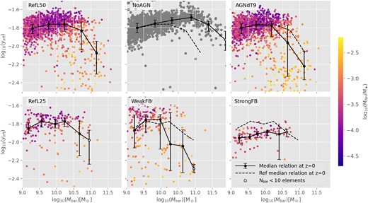
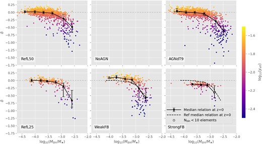
Mbar–yeff relation colour-coded according to the ratio between BH and stellar mass (MBH/M⋆) for z = 0 eagle galaxies. The top (bottom) panels show results for models with different AGN (SN) feedback parameters (see Table 1, for details), as indicated in the legend. The solid lines represent the z = 0 median relation, and the dotted lines in the middle and left panels depict the z = 0 median relation for the reference model. The error bars denote the 25th and 75th percentiles. Mass bins populated with less than 10 elements (Nbin < 10) are marked with white circles.
According to the top panels in Fig. 1 and consistently with results from LL19, variations of the AGN feedback model affect mostly yeff of massive galaxies (Mbar ≳ 1010 M⊙). At low masses, where MBH/M⋆ ≲ 10−3.5 for the bulk population, all simulations predict similar weak yeff–Mbar correlations with low scatter and high yeff. At higher Mbar ≳ 1010 M⊙, the NoAGN model predicts the highest yeff at a given mass. On the other hand, the RefL50 and AGNdT9 models predict a strong median decrease of yeff with Mbar, caused by the presence of massive galaxies with dominant BH (MBH/M⋆ ≳ 10−3.5) and very low yeff. The scatter at high masses also increases with ΔTAGN. For the RefL50 and AGNdT9 simulations, the low yeff of massive galaxies can be associated with the accumulated impact of AGN feedback driven by their dominant BH, which can heat SF gas, suppress star formation and chemical evolution, and drive outflows of metal-enriched material out of galaxies (see De Rossi et al. 2017 and LL19, for a discussion). Thus, our findings suggest a close connection between yeff and MBH/M⋆.
The effects of varying the SN feedback efficiency are presented in the bottom panels of Fig. 1. In the case of the strong SN feedback model, all galaxies show low MBH/M⋆ and yeff, which are below those corresponding to systems of similar masses in the RefL25 model. On the other hand, the WeakFB model predicts a higher percentage of galaxies with high MBH/M⋆ at all masses. At low masses, the WeakFB and RefL25 models predict similar median yeff–Mbar relations, whereas, at higher masses, the WeakFB simulation shows a stronger yeff–Mbar anticorrelation, as a consequence of the higher number of galaxies with dominant BH. The WeakFB model also predicts a larger scatter. Hence, it is important to highlight that the impact of SN feedback extends beyond the direct removal of metal-enriched material, as observed in the StrongFB simulation. SN feedback also appears to affect yeff through the regulation of the BH-to-stellar mass growth: interestingly, a weaker SN feedback tends to drive a more pronounced impact from AGN feedback, whereas a stronger SN feedback diminishes the relevance of AGN feedback. As already discussed by Henriques et al. (2019), SN feedback has a critical role in regulating the efficiency of AGN feedback; when the stellar mass reached by the galaxy is large enough to avoid mass ejection by SN feedback, more cold gas becomes available for star formation and BH growth, thus giving place to AGN feedback.
According to the aforementioned findings, both SN and AGN feedback seem to affect the shape, normalization, and scatter of the yeff–Mbar relation in different ways, which suggests that its features can provide clues about the relative accumulated effects of feedback in real galaxies of different masses. Considering the predictions of our simulations, (1) at a given |$M_{\rm bar }\gtrsim 10^{10}~{\rm M}_{\odot }$|, lower yeff can be associated with a stronger impact of AGN feedback, (2) at a given |$M_{\rm bar }\lesssim 10^{10}~{\rm M}_{\odot }$|, galaxies with higher than the median yeff can be associated with a weaker SN feedback efficiency and a weaker AGN feedback impact, and (3) at a given |$M_{\rm bar }\lesssim 10^{10}~{\rm M}_{\odot }$|, galaxies with yeff well below the median correspond generally to systems with a strong AGN impact and a weak SN feedback efficiency.
Finally, we note that some previous works that analyse eagle galaxies in the context of analytical models adopt a ‘true stellar yield’ parameter yZ = 0.04 [log10(yZ) ≈ −1.4; e.g. Sharma & Theuns 2020; Zenocratti et al. 2022], which seems to be suitable for describing the behaviour of most simulated systems. Such value is consistent with the net yields expected for simple stellar populations (SSPs) with a Chabrier IMF (e.g. Madau & Dickinson 2014). The effective yields shown in Fig. 1 are below the aforementioned true yield parameter, a fact that is expected as simulated galaxies are not closed boxes. In addition to SN and AGN feedback, they are affected by the accumulated effects of past mergers and gas flows. Besides, simulated galaxies are composed by a mix of SSPs with different metallicities and, thus, different net yields.
3.2 Metallicities, stellar masses, and gas fractions
As effective yields are calculated from metallicities, stellar masses, and gas fractions (equation 2), the study of feedback effects on such quantities is relevant to explain their impact on yeff. In this section, we start exploring well-known 2D galaxy scaling relations involving O/H, M⋆, and μ. Consequences of varying AGN and SN feedback models on such relations are analysed in Figs 2 and 3, respectively, where scatter plots are colour-coded by yeff, and symbols are scaled to the value of MBH/M⋆.

Simulations that evaluate the effects of varying the AGN feedback model (see Table 1, for details). Left panels: M⋆–O/H relation. Middle panels: M⋆–μ relation. Right panels: μ–O/H relation. The connection between each of these relations and the effective yields is highlighted by colour-coding symbols according to the values of yeff. Symbols are also scaled to the value of MBH/M⋆. The solid lines represent the z = 0 median relation, and the dotted lines in lower panels depict the z = 0 median relation for the reference model. The error bars denote the 25th and 75th percentiles. Mass bins populated with less than 10 elements (Nbin < 10) are marked with white circles.
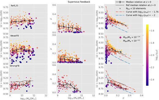
Simulations that evaluate the effects of varying SN efficiency (see Table 1, for details). Left panels: M⋆–O/H relation. Middle panels: M⋆–μ relation. Right panels: μ–O/H relation. The connection between each of these relations and the effective yields is highlighted by colour-coding symbols according to the values of yeff. Symbols are also scaled to the value of MBH/M⋆. The solid lines represent the z = 0 median relation, and the dotted lines in lower panels depict the z = 0 median relation for the reference model. The error bars denote the 25th and 75th percentiles. Mass bins populated with less than 10 elements (Nbin < 10) are marked with white circles.
3.2.1 AGN feedback effects
The left panels of Fig. 2 show the M⋆ZgR for different AGN feedback models. At the low-mass end, different feedback prescriptions predict high yeff and a slightly similar positive M⋆ZgR slope. We notice a break-point at M⋆ ∼ 1010.3M⊙, where the RefL50 and AGNdT9 models predict a transition from a correlation to an anticorrelation for higher masses. On the other hand, a steeper correlation is obtained for the NoAGN model at such intermediate masses, with a gradual flattening towards M⋆ ≳ 1011.5 M⊙. The steeper negative slope of the high-mass end of the M⋆ZgR with increasing ΔTAGN is accompanied by an increasing number of metal-poor galaxies with low yeff. In fact, comparing the three simulations, galaxies with the lowest yeff are obtained in the RefL50 and AGNdT9 implementations, and correspond to systems with high M⋆ and low O/H. In addition, the scatter plots symbols in Fig. 2 are scaled with MBH/M⋆. It is clear that massive galaxies with lower metallicities have more dominant BHs, indicating that they could have been more affected by AGN feedback. On the contrary, we note that the highest values of yeff are obtained in the simulation NoAGN and correspond to systems with low M⋆, high O/H, and null MBH/M⋆. Our findings are in agreement with De Rossi et al. (2017), who claimed that the negative slope of the M⋆ZgR at high M⋆ can be driven by AGN feedback through two different main channels: (i) the heating of SF gas and its subsequent change to a non-star-forming (NSF) phase, which drives the quenching of star formation and, consequently, the suppression of chemical evolution; (ii) the ejection of metal-enriched gas out of galaxies. yeff seem to be good tracers of this situation, reaching lower and lower values as the global metallicity decreases due to the increasing AGN feedback influence.
As seen in the middle panels of Fig. 2, all AGN feedback models generate similar median M⋆–μ anticorrelations, with μ ranging between 0 and 0.5 for smaller galaxies, and showing almost negligible values, for massive ones. Although weaker, there is a trend for massive galaxies of decreasing their SF gas fraction with increasing ΔTAGN. Such a behaviour is expected given that AGN feedback heats the gas, fostering its transition to an NSF phase. It is also worth noting that, as ΔTAGN increases, there is a higher number of galaxies with low yeff and very low μ, specially for high-mass galaxies. Therefore, considering equation (2) and our previous analysis of the M⋆ZgR, the lower yeff at the high-mass end are a consequence of both the lower μ and lower metallicity of the corresponding galaxies.
Finally, the right panels of Fig. 2 show the μ–O/H relation. Consistently with the findings of De Rossi et al. (2017) for the eagle ‘Recal’ model, our simulations predict a tight decrease of metallicity with increasing SF gas fraction, showing a larger scatter towards lower values of μ. Typical galaxies with |$\mu \gtrsim 0.1$| depict a median relation that follows roughly a curve corresponding to a constant log10(yeff) ≈ −1.76. Interestingly, such tight relation represents well the behaviour of galaxies derived from our three different AGN feedback models, with the only exception of gas-poor systems. In particular, when AGN feedback is turned off, a higher number of gas-poor systems show higher metallicities and yeff. On the other hand, the RefL50 model predicts a significant population of gas-poor systems with lower than average metallicity and lower than average yeff. And, the latter population is even larger for the AGNdT9 model. As shown before, very low yeff are related to the presence of galaxies with dominant BH (i.e. high MBH/M⋆ values) and, hence, probably more affected by AGN feedback. In particular, three ranges of yeff are clearly distinguished in the μ–O/H plane: (1) galaxies with high yeff follow the log10(yeff) ≈ −1.76-curve, showing slightly higher than average metallicity at a given μ; (2) galaxies with intermediate yeff also follow the same curve, showing slightly lower than average metallicity at a given μ; (3) low yeff correspond to galaxies with low metallicities and low gas fractions, significantly departing from the log10(yeff) ≈ −1.76-curve. The latter region is only significantly populated when AGN feedback is turned on and corresponds to massive galaxies (|$M_\star \gtrsim 10^{10}~\rm {M}_\odot$|) with the most dominant BHs.
3.2.2 SN feedback effects
In this section, we explore the effects of varying SN feedback efficiency on O/H, M⋆, and μ. Given the smaller box of the simulations analysed here (RefL25, WeakFB, StrongFB; see Section 2), the number of galaxies in our selected samples is smaller than those studied in the previous section (RefL50, NoAGN, AGNdT9; see Table 1). We also note that, in the case of the StrongFB simulation, the number of galaxies is a factor of ≈2 lower than for the WeakFB run (Table 1). This is related to the stronger efficiency of feedback in the former case, which leads to a decrease in the star formation of galaxies due to gas heating and SN-driven winds. These effects prevent that many galaxies surpass our imposed lower mass limit of M⋆ = 109 M⊙.
In Fig. 3 (left panels), the effects of different SN feedback prescriptions on the M⋆ZgR are compared. We clearly see distinct patterns for the different simulations. As reported in previous works, the RefL25 model predicts a flat median relation with moderate scatter. Regarding the WeakFB model, it leads to a higher normalization for the median M⋆ZgR, which shows slightly higher positive (negative) slope at low (high) M⋆. The WeakFB model also produces a larger scatter in metallicity at all masses. Such scatter is mostly generated by the appearance of a population of galaxies with low metallicities, low yeff, and dominant BHs (larger symbols, see also Fig. 1). But, in contrast with RefL50 and AGNdT9 simulations (see Fig. 3), a significant number of dominant BHs are located in low-mass galaxies in the WeakFB simulation. This could be caused by the weaker SN efficiencies in the latter case, which allows more gas to cool down and reach the galaxy centre, enhancing the growth of the central BH (see, also, the discussion in Section 3.1). According to these results, a weak feedback efficiency can lead to significant AGN feedback impact in galaxies of all masses, contributing to lower metallicity even for low-mass systems. On the other hand, the StrongFB model do not lead to the formation of dominant BHs, driving an M⋆ZgR with a positive slope along the whole mass range. These trends support again a scenario where dominant BHs are required for reproducing the flattening of the M⋆ZgR at high masses (De Rossi et al. 2017). In addition, the normalization of the M⋆ZgR is lower for the StrongFB model, which is expected as a stronger SN feedback fosters the ejection of metal-enriched material out of galaxies.
In the middle panels of Fig. 3, we compare the μ–M⋆ relation for our three SN feedback scenarios. In the case of the reference model, μ decreases with increasing M⋆, with a large scatter around the median relation. Low values of yeff can be associated with gas-poor galaxies. A similar behaviour is obtained for the WeakFB model but, with a lower normalization for μ, and a higher number of gas-poor galaxies with low yeff. This is consistent with a more efficient SF process and gas consumption in the WeakFB simulation: given the less significant influence of SN feedback, galaxies tend to form their stellar component earlier. In addition, as previously discussed, low-yeff galaxies in these simulations also have dominant BHs, which prevent further gas cooling, quenching star formation, and chemical evolution. It is interesting to see that only systems with dominant BHs reach negligible μ. In the case of the StrongFB simulations and contrary to expectations, low-mass galaxies show higher median μ than in the other simulations. This can be due to a stronger SN feedback heating during the peak of the SF histories of these systems, which could cause the ejection of gas from the shallower potential well of these galaxies, with the ejected material remaining in the outer part of them. As the potential wells become deeper at later epochs, the ejected material could have been re-accreted, driving an increase in μ and a decrease in metallicity; this explains the presence of a more significant population of galaxies with low O/H and high μ in the StrongFB simulation.
With respect to the μ–O/H relation (Fig. 3, right panels), the RefL25 model predicts similar trends to those discussed before for the RefL50 simulation: O/H decreases with increasing μ, a larger scatter is obtained at lower μ, and, once more, the median μ–O/H relation follows a curve of constant log10(yeff) ≈ −1.76. But, in contrast to the results obtained from variations of ΔTAGN, variations in SN feedback efficiencies generate more significant departures from the log10(yeff) ≈ −1.76 curve. For the WeakFB model, the μ–O/H relation is flatter, shows larger scatter, and exhibits a small offset towards higher metallicities (and, hence, higher yeff) with respect to the RefL25 model. On the other hand, for the StrongFB model, the μ–O/H relation presents a similar slope to that associated with the RefL25 model, but departs around 0.2 dex towards lower metallicities (following roughly the curve of constant log10(yeff) ∼ −2).
3.3 Effective yield-BH connection
The results obtained so far suggest the existence of an anticorrelation between yeff and MBH/M⋆. This is verified in Fig. 4, which presents a scatter plot of the dependence of yeff on MBH/M⋆ for all models considered. Note that symbols are colour-coded according to M⋆.
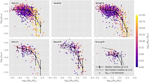
yeff versus MBH/M⋆ for different AGN (top panels) and SN (bottom panels) feedback models (see Table 1, for details). Symbols are colour-coded according to M⋆. The solid curves correspond to the median relations and the error bars depict the 25th and 75th percentiles. For the sake of comparison, the median relation corresponding to the reference model for each simulation set is shown in each panel.
It is clear that, for galaxies with high MBH/M⋆ ≳ 10−3.5, all simulations predict a strong anticorrelation between yeff and MBH/M⋆. Although the median yeff–MBH/M⋆ relation seems not to depend on the feedback model, the number of galaxies with higher MBH/M⋆ increases for higher AGN heating temperatures. Besides, galaxies with MBH/M⋆ ≳ 10−3.5 tend to have M⋆ ≳ 1010 M⊙ in all simulations, with the only exception of the WeakFB run. For the latter model, lower mass galaxies can have dominant BHs, as we showed before. Our results indicate that AGN feedback seems to be mainly responsible for the decrease of yeff as MBH/M⋆ increases at |$M_{\rm BH}/M_{\star } \gtrsim 10^{-3.5}$|.
On the other hand, SN feedback has an influence on the BH growth through the regulation of the gas reservoir. Clear signatures of SN feedback impact on yeff are evident at low MBH/M⋆, where lower M⋆ and an almost constant yeff value are obtained for all simulations. At MBH/M⋆ ≲ 10−3.5, the StrongFB and WeakFB models predict a median yeff of ∼10−1.9 and ∼10−1.7, respectively. On the other hand, the reference and AGNdT9 models show, for similar MBH/M⋆, yeff ∼ 10−1.76, which corresponds to the median yeff for the NoAGN case. Additionally, it is interesting to note that the StrongFB model predicts yeff within a narrow range of intermediate values (≈10−2.2–10−1.8) for almost all galaxies, compared with the wider range of yeff values covered by other feedback models (≈10−2.4–10−1.6). Our trends could be explained considering that a strong SN feedback efficiency prevents from reaching very high yeff, whereas the lack of very massive BHs (required for a strong AGN feedback impact), in the case of a strong SN feedback, prevents from reaching very low yeff. To sum up, Fig. 4 suggests that, in the case of galaxies with no dominant BH, yeff seem to be mostly determined by the efficiency of SN feedback, while, for galaxies with dominant BH, yeff show a strong anticorrelation with MBH/M⋆ due, mainly, to AGN feedback.
Finally, we note that the MBH/M⋆ range obtained from our analysis is consistent with recent observations of massive galaxies (e.g. Graham & Sahu 2023). This is not a surprise as the reference model in eagle simulations was calibrated using the relation between BH mass and stellar mass in a similar mass range (Section 2).
Summarizing the results from Section 3, AGN feedback tends to favour the simultaneous decrease of the SF gas fraction and metallicity of high-mass galaxies, leading to lower yeff. On the other hand, a stronger SN feedback efficiency leads to lower yeff at all stellar masses as a consequence of the decrease of metallicity at a given SF gas fraction. And, a weak SN feedback efficiency drives a more complex behaviour, fostering the formation of dominant BHs for a significant number of galaxies even at low M⋆: galaxies with dominant BH show lower O/H, lower SF gas fractions and, hence, lower yeff, while galaxies with low MBH/M⋆ exhibit higher metallicities at a given SF gas fraction, and, hence, higher yeff.
4 THE STELLAR MASS–METALLICITY–GAS MASS PARAMETER SPACE
Lara-López et al. (2010) found a fundamental metallicity plane for SF galaxies, relating SFR, M⋆, and O/H (see also Ellison et al. 2008; Mannucci et al. 2010). Considering the results reported by Lara-López et al. (2013), such a plane could be a consequence of an underlying relation between M⋆, O/H, and μ (see also Bothwell et al. 2013 for another observational work and, e.g. Lagos et al. 2016 and De Rossi et al. 2017 for related analysis using eagle simulations). As yeff are defined from these key galaxy properties and taking into account the results discussed in the previous section, it is reasonable to expect that yeff could trace the impact of feedback processes on the features of the aforementioned 3D galaxy metallicity scaling relations. In this section, we examine the relation between M⋆, |${\rm 12+\log _{10}({\rm O/H})}$| and Mgas (hereafter, M⋆, gZgR), for our complete set of eagle simulations. We aim at evaluating how feedback processes affect the relations between these three fundamental properties and try to assess the role of yeff as a feedback indicator.
Figs 5 and 6 show the M⋆, gZgR for simulations with different AGN and SN feedback prescriptions, respectively. Different symbols are colour-coded according to MBH/M⋆. For the NoAGN simulation, MBH is always zero so galaxies are shown with an uniform grey colour. Comparing results from different panels, we see that AGNdT9 and WeakFB simulations present the largest dispersion. On the other hand, the smallest dispersion is obtained for the NoAGN simulation, which, indeed, predicts an M⋆, gZgR that can be well represented by a plane. Such NoAGN plane also seems to be a good representation of the bulk of galaxies with no dominant BH (i.e. low MBH/M⋆) in other simulations.
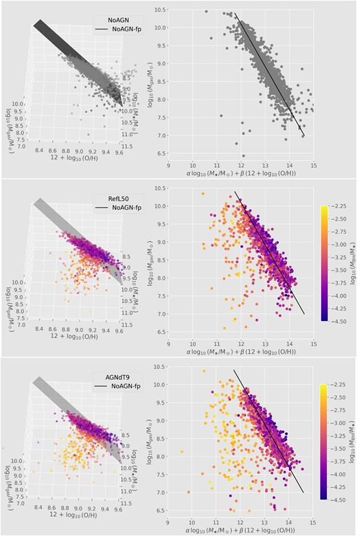
Scatter plot of galaxies in the M⋆–O/H–Mgas space for simulations that evaluate the effects of varying AGN feedback (see Table 1, for details). Left panel: 3D visualization. Right panel: 2D projection with α = −1 and β = C2 = 2.49. Symbols are colour-coded with MBH/M⋆ as an indicator of the dominance of the BH mass in each galaxy. Note that, for the NoAGN simulation, MBH is null for all galaxies, so they are shown with an uniform grey colour. For more viewing angles, see the Supplementary Material.

Similar to Fig. 5, but for the simulations that evaluate the effects of varying SN efficiency (see Table 1, for details). For more viewing angles, see the Supplementary Material.
We determined the characteristic plane associated with the NoAGN model by performing a least-square fit, of a second-order polynomial, with the R hyperplane fitting package hyper-fit (Robotham & Obreschkow 2015). The plane is well described by the following expression:
where the parameters C1, C2, and C3 are shown in Table 2 for different data samples. The first row in the table corresponds to the plane plotted in Figs 5 and 6, and discussed here. We will refer to this plane as the NoAGN fitting plane (hereafter, ‘NoAGN-fp’).
Output parameters (C1, C2, and C3; fifth to seventh columns, respectively) from the fitting of equation (4) to the NoAGN simulated sample, as indicated in the first column. The 2D plane fit of the 3D data was performed using the R package hyper-fit (Robotham & Obreschkow 2015). The eighth column indicates the intrinsic scatter orthogonal to the hyperplane (ϵ). The second column indicates the stellar component used in the calculations: total stellar mass or stellar mass used in LL19 (i.e. the component enclosed within a radius of 30 kpc, for simulations). The third column shows the considered gas component: total gas component, total SF gas phase, or the gas component used in LL19 (i.e. total hydrogen mass enclosed within a radius of 70 kpc, for simulations). The fourth column indicates the gas component used for estimates of O/H: total gas component, total SF gas phase, or that used in LL19 (i.e. SF gas within a radius of 30 kpc, for simulations).
| Data sample | Stellar mass | Gas mass | Gas metallicity | C1 | C2 | C3 | ϵ | Plane identifier |
|---|---|---|---|---|---|---|---|---|
| NoAGN simulation | total | total SF | total SF | 0.844 (± 0.013) | 2.49 (± 0.05) | −20.5 (± 0.5) | 0.320 | NoAGN-fp |
| NoAGN simulation | total | total | total | 0.949 (± 0.010) | 1.35 (± 0.02) | −11.0 (± 0.2) | 0.248 | NoAGN-fp-tot-gas |
| NoAGN simulation | LL19 | LL19 | LL19 | 0.773 (± 0.011) | 2.59 (± 0.04) | −21.1 (± 0.4) | 0.299 | NoAGN-fp-LL19 |
The departures (residuals) from the NoAGN-fp can be quantified by calculating the orthogonal deviation of each galaxy i from such a plane as
where the subscript i indicates quantities corresponding to the given galaxy i.
For the sake of clarity, the following convention will be adopted in this work: at a fixed M⋆ and O/H, galaxies with higher (lower) Mgas than the value corresponding to the NoAGN-fp are assumed to be located ‘over’ (‘under’) the plane, presenting positive (negative) deviations with respect to it.
A comparison between the NoAGN-fp and the features of the M⋆, gZgR for different feedback models is carried out in Section 4.1. In Section 4.2, we analyse the connection between the latter findings and the distribution of yeff values for galaxy populations in different simulations. In Section 4.3, we evaluate how different feedback scenarios can affect the deviations of the M⋆, gZgR from the NoAGN-fp.
4.1 Feedback impact on the M⋆, gZgR
In Figs 5 and 6, we compare the best-fitting plane obtained for the NoAGN simulation (grey surface) with the M⋆, gZgR associated with different feedback models. We see that the NoAGN-fp can roughly describe the behaviour of the vast majority of galaxies with no dominant BH. In addition, when varying SN or AGN feedback prescriptions, clear distinct trends are obtained for the location of galaxies with respect to the NoAGN-fp.
Fig. 5 evaluates the impact of AGN feedback on the M⋆, gZgR. As previously discussed, the increase of ΔTAGN leads to a more significant number of galaxies with higher MBH/M⋆. At the same time, the AGNdT9 model predicts the highest number of galaxies spread below the NoAGN-fp, displaying also the most substantial negative deviations. Another key feature is the dependence of the distance to the plane on the dominance of the BH, which is quantified by the parameter MBH/M⋆. Galaxies with lower MBH/M⋆ tend to be located closer to the plane, with almost null deviations with respect to it or even slightly positive ones. Conversely, systems with higher MBH/M⋆ show larger negative deviations. Therefore, our findings suggest that galaxies tend to deviate down from the NoAGN-fp as they are more affected by the heating of gas by AGN feedback.
The consequences of varying SN feedback are analysed in Fig. 6. In principle, we can clearly see that a change in the SN feedback efficiency affects not only the scatter of the M⋆, gZgR but also the displacement of the bulk of the galaxy population with respect to the NoAGN-fp. For the StrongFB model, all galaxies tend to be located below the NoAGN-fp. As discussed before, a stronger SN feedback leads to a moderate average decrease in O/H, at a given μ, for most of the galaxies (Section 3), which explains their moderate displacement down the NoAGN-fp. For such galaxies, MBH/M⋆ ∼ 10−4–10−3, which are values well below the maximum ones reached by galaxies in other simulations (MBH/M⋆ ∼ 10−2.5–10−2). Thus, in the case of the StrongFB model, larger deviations from the NoAGN-fp are not possible given that AGN feedback effects seem to be limited. As SN feedback efficiency decreases (see plots corresponding to the simulation WeakFB), most of the galaxies move, on average, closer to the NoAGN-fp, some of them reaching positive deviations with respect to it. It is interesting to highlight that, in the WeakFB simulation, galaxies above the NoAGN-fp (purple galaxies) are those characterized by low values of MBH/M⋆ (|$\lesssim 10^{-3.5}$|). Thus, these galaxies more closely resemble a closed box model for two main reasons. First, the low SN feedback efficiency implemented in this model ensures a weak effect of stellar winds and energy injection due to SN feedback. Secondly, the low values of MBH/M⋆ indicate that they should not have been strongly affected by gas outflows caused by AGN feedback. On the other hand, the WeakFB model also predicts a significant number of galaxies with high MBH/M⋆, which tend to be located at larger distances below the NoAGN-fp. As mentioned before, SN and AGN feedback processes seem to be indirectly intertwined for such galaxies: due to their lower SN feedback efficiency, they could have evolved faster due to an early efficient consumption of their cold gas reservoir, reaching z = 0 with higher MBH/M⋆ and, thus, having been more affected by AGN feedback.
A comprehensive analysis of the differences between galaxies in proximity to the NoAGN-fp and those situated at greater distances is undertaken in greater depth within Section 5.1.
4.2 Effective yields as feedback tracers
To evaluate the connection between yeff and the feedback-driven features of the M⋆, gZgR in Figs 5 and 6, we can compare the M⋆, gZgR predicted by different feedback models with the yeff distribution of simulated galaxies. In this sense, we note that, since yeff is given by gas metallicity and gas mass fraction (equation 2), a unique yeff value is associated with each point within the 3D parameter space defined by M⋆, O/H, and Mgas. Interestingly, simulated galaxies located around the NoAGN-fp show a roughly constant yeff ≈ 10−1.76, being these trends consistent with the flatter Mbar–yeff relation described by galaxies in the NoAGN simulation (see Fig. 1). Such characteristic value yeff ≈ 10−1.76 approximates the average yeff of galaxies in the NoAGN model. In addition, the bulk of the galaxy population in all simulations is located within a region where the NoAGN-fp seems to be a good local representation of a surface defined by yeff ≈ 10−1.76. In this context, orthogonal deviations from the NoAGN-fp in our 3D parameter space can be associated, locally, with variations in the values of yeff. As we will show in next section, the highest yeff are reached by those galaxies with the largest positive deviations with respect to the plane, which correspond to systems with lower MBH/M⋆. On the other hand, galaxies that are located under the NoAGN-fp plane with larger deviations from it show higher MBH/M⋆ and lower yeff (see, also, Fig. 4).
It is important to remember that our galaxy samples include both central and satellite galaxies of haloes (Section 2.2). We verify that similar general trends would be obtained if only central galaxies were considered for our analysis; specially, a similar NoAGN-fp would emerge since few satellites lie within the considered mass range in the NoAGN simulation. Satellite galaxies only tend to increase the dispersion towards lower masses as a consequence of the presence of systems with high yeff. This is consistent with the enhanced metallicity of eagle satellite galaxies reported by Bahé et al. (2017). These authors studied the eagle reference model and concluded that satellite galaxies tend to be more metal-enriched than equally massive centrals. They demonstrated that this phenomenon is primarily driven by the removal of metal-poor SF gas from the outer regions of galaxies, accompanied by the suppression of metal-poor inflows resulting from the removal of gas from the galaxy halo. Consequently, satellite galaxies in eagle simulations present higher metallicities than central galaxies of the same mass, showing positive deviations from the NoAGN-fp.
4.3 Residual analysis
In this section, we quantify the deviations from the NoAGN-fp using the residuals δ defined in equation (5). We remind that, at a given M⋆ and metallicity, δ is taken to be positive (negative) for higher (lower) values of Mgas with respect to the NoAGN-fp.
Fig. 7 shows δ as a function of MBH/M⋆ for different feedback models. Symbols are colour-coded according to yeff. For models including the reference SN feedback efficiency (RefL25, RefL50, AGNdT9), galaxies with less dominant BHs (|$M_{\rm BH}/M_{\star } \lesssim 10^{-3.5}$|) show negligible median residuals. This is expected since the NoAGN feedback model, from which the NoAGN-fp is derived, adopts a reference SN feedback efficiency and considers no AGN feedback effects; hence, such a behaviour should be recovered for galaxies with low MBH/M⋆ in simulations with the default SN feedback model. On the other hand, for galaxies with no dominant BH, the residuals become negative (positive) when implementing a stronger (weaker) SN feedback efficiency relative to the reference model. In the case of galaxies with more dominant BH (MBH/M⋆ ≳ 10−3.5), δ decreases with MBH/M⋆ in all simulations, as it is also evident from Figs 5 and 6; this is a consequence of the increasing relevance of AGN feedback.
Residuals from the NoAGN-fp, δ, versus log10(MBH/M⋆), colour-coded with yeff. The top (bottom) panels compare different AGN (SN) feedback models (see Table 1, for details). The horizontal dotted lines highlight the null distance to the NoAGN-fp. Note that for the NoAGN model, MBH is null, so no galaxies are plotted in this case.
The tight relation between yeff and δ is clear in Fig. 7 (compare it, also, with Fig. 4), which can be well described by a linear function, as we checked. By performing a linear least squares fit to the data obtained in the NoAGN model, this relation takes the form
being valid for galaxies in all simulations. As discussed before, the NoAGN-fp locally represents a surface of constant yeff in our 3D parameter space. δ measures the length of an orthogonal vector from the plane to a given galaxy, so that this vector should be parallel to the gradient of the scalar field defined by yeff. Hence, increasing δ, implies continuously crossing isosurfaces associated with different yeff values.
5 DISCUSSION
Our results suggest a close connection between the accumulated effects of AGN and SN feedback, and the features of scaling relations involving stellar mass, metallicity, and gas mass. In addition, given that yeff is defined from those quantities, it seems to be a good tracer to constrain different feedback scenarios. In particular, we detect a characteristic plane in the 3D parameter space defined by the aforementioned properties, which is surrounded by galaxies with a reference SN feedback and a negligible impact of AGN feedback. Interestingly, the plane locally describes a surface of constant yeff, so that orthogonal departures from the plane can be directly associated with variations in yeff (i.e. different yeff isosurfaces are crossed when moving away from the plane). An increasing influence of SN or AGN feedback generates deviations towards lower yeff. On the other hand, a weaker SN feedback can only drive positive variations of yeff for galaxies not significantly affected by AGN (i.e. with low MBH/M⋆); in other case, AGN feedback causes the decrease of yeff.
In this section, we discuss about the nature of our findings and their implications. We also explore our results in the context of observational data.
5.1 The nature of deviations from the NoAGN-fp
In this section, we try to get more insight into the nature of the residuals (δ, see equation 5) from the NoAGN-fp (Section 4), which, in principle, seem to be strongly dependent on the dominance of the BH inside galaxies (Fig. 7). Our aim is to explore plausible important mechanisms that can enhance the growth of the BH mass in our selected galaxies and lead to such deviations.
We address the impact of merger events by analysing the formation histories of galaxies studied in the preceding sections. For this analysis, we consider mergers experienced by the main progenitor branch3 of each galaxy selected at z = 0. The results are summarized in Fig. 8, where δ is plotted against the total baryonic mass (including the stellar, SF gas, and NSF gas components) accumulated through merger events (i.e. Mtot, accr = ∑iMbar, tot, i, where i considers all satellites that merge onto the main progenitor along the galaxy evolution). The upper panel corresponds to simulations which adopt different SN feedback efficiencies, while the lower panel examines the impact of implementing different temperature increases due to AGN feedback.

Residuals (δ) from the NoAGN-fp as a function of the total mass (stars + SF gas + NSF gas) accreted via merger events, colour-coded by the dominance of BH, for models that varies the efficiency of SN feedback (top panel) and AGN feedback (bottom panel) (see Table 1, for details). The curves represent the median relations, and the error bars denote the 25th and 75th percentiles. Symbols corresponding to the NoAGN simulation are coloured grey, since the variable MBH/M⋆ is null for all galaxies in this model.
With the exception of the StrongFB model, a consistent trend appears across the majority of models. Notably, we observe that galaxies with larger negative δ have acquired a more significant amount of baryonic mass through merger events. In addition, a more close inspection suggests also that these galaxy mergers have driven the accretion of gas and BH growth in simulated systems, which reach z = 0 with more than 80 per cent of the total baryonic mass and more than 40 per cent of the total gas in the form of NSF gas. These findings are in agreement with the higher MBH/M⋆ shown by galaxies with δ < 0: merger events can supply significant amounts of gas and potentially generate instabilities which can lead to the migration of material towards the inner galaxy regions, hence boosting the gas accretion rate onto BHs and the injection of energy via AGN feedback. Moreover, mergers between BHs can take place during galaxy mergers, leading to an increase in the BH mass of the remnant systems. This behaviour is not seen in the case of the StrongFB model, likely due to the lower baryonic masses reached by galaxies in this sample (see Fig. 1); merger events are expected to have had a more significant role on the formation of more massive galaxies.
We also analysed the BH accretion rates in our z = 0 galaxies, |$\dot{M}_{\rm BH,accr \, (z=0)}$|, and the median of this quantity along the galaxy lifetime calculated along the main branch of progenitors of each galaxy, |$\langle \dot{M}_{\rm BH,accr \, (z)} \rangle$|.4 The former provides information regarding the current state of the BH, while the latter gives us details about the historical value of the BH accretion rate of each galaxy (see Section 2.1.3, for further details). This information is plotted in Fig. 9. It is clear that, for all models, galaxies with higher MBH/M⋆ tend to show a stronger present and past average BH activity, confirming that such systems have been more significantly affected by AGN feedback.
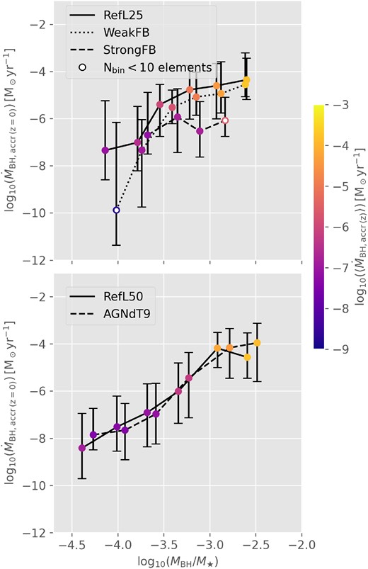
BH accretion rate at z = 0 versus MBH/M⋆, colour-coded by the median BH accretion rate along the galaxy lifetime calculated for the main branch of each galaxy, for models that varies the efficiency of SN feedback (top panel) and AGN feedback (bottom panel) (see Table 1, for details). The curves represent the median relations, and the error bars denote the 25th and 75th percentiles. No data are plotted for the NoAGN simulation due to the null values of MBH for all galaxies in this model.
5.2 Gas heating impact on effective yields
AGN and SN feedback can affect the gas component of galaxies through two main channels: (1) gas heating, which could quench the star formation and, hence, the chemical evolution of galaxies; (2) metal-enriched gas outflows, which deprive the galaxies from fuel for forming new stars and lower the metallicity of the systems (see De Rossi et al. 2017, for a discussion about these effects in eagle). So far, we have defined all our gas quantities considering only the SF gas component of galaxies (Section 2.2), which can vary through the two aforementioned mechanisms. But, a close inspection of our galaxy sample in different simulations reveals that galaxies below the NoAGN-fp tend to have significantly high percentages of NSF gas (≳85 per cent, for the majority of galaxies). On the other hand, galaxies above the plane, which show the highest yeff, tend to have lower amounts of NSF gas. These findings suggest that feedback-driven gas heating is probably the main process responsible for yeff negative variations and deviations down the NoAGN-fp. In this context, it is interesting to explore the behaviour of galaxies if re-defining gas properties in order to include the NSF phase. Thus, we re-estimated all our galaxy properties considering the whole gas component (including SF and NSF gas) within each system. Gas heating can foster the transition from the SF to the NSF gas phase, affecting quantities derived from SF gas, while, by definition, the total gas component is not affected by such transition. Thus, the analysis of the variations of the latter component with feedback allows to probe the relevance of gas heating against that of outflows.
In Fig. 10, we analyse the 3D distribution of galaxies in the parameter space given by the total gas mass (Mgas, tot = Mgas, SF + Mgas, NSF, where Mgas, NSF stands for the NSF gas component), M⋆, and oxygen abundance derived from the total gas component (O/H)tot. Symbols are colour-coded with yeff, tot = Zgas, tot/ln (1/μtot), where Zgas, tot is the metallicity corresponding to the whole gas phase and μtot = Mgas, tot/(M⋆ + Mgas, tot). The left and right panels show results for the NoAGN and RefL50 models, respectively. We see that, when taking into account the total gas component, galaxies in the NoAGN simulation are again located around a plane (NoAGN-fp-tot-gas, hereafter), showing even lower dispersion around the plane than that obtained in Figs 5 and 6. The new output parameters from the fitting of equation (4) to the NoAGN simulated sample and the corresponding scatter can be found in Table 2 (second row).
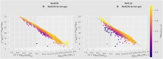
3D scatter plot of galaxies in the |$M_{\star }-{\rm (O/H)_{\rm tot}}-M_{\rm gas,tot}$| space for the NoAGN (left-hand panel) and RefL50 (right-hand panel) simulations (see Table 1, for details), colour-coded with yeff, tot. All quantities are calculated using the total gas component. The grey shadow represents the fitting plane obtained from the NoAGN simulation. More viewing angles are available in the Supplementary Material.
The right panel of Fig. 10 shows the M⋆, gZgR for the RefL50 simulation. We see that, when using the whole gas component for defining our properties, negative deviations from the plane decrease significantly. In fact, the NoAGN-fp-tot-gas seems to constitute a good representation for almost all the galaxy population even for the RefL50 model, with very few systems exhibiting very negative departures. A more in-depth examination of the latter simulation reveals that, for galaxies exhibiting the highest MBH/M⋆ ratios, the median deviation from the NoAGN-fp is δ ≈ −0.5 when calculating properties solely from the SF gas component. Conversely, when calculating properties from the whole gas component, the median departure from the NoAGN-fp-tot-gas is δ ≈ −0.25, consistent with the smaller scatter around the plane (see Table 2). These results are in line with feedback-driven gas heating (which fosters the transition from the SF to the NSF gas phase), being mainly responsible for the negative deviations from the NoAGN-fp (and the associated decrease of effective yields) in Figs 5 and 6.
Finally, we emphasize that findings from this section do not imply that galaxies roughly behave as closed-boxes when taking into account their whole gas component. All simulated galaxies are affected by gas inflows, outflows, and mergers during their evolution. Our results point out the importance of the criteria used for characterizing the gas phase for the correct use of yeff as a tracer of feedback impact on metallicity scaling relations.
5.3 Comparison with observations
LL19 performed a detailed comparison between effective yields in eagle simulations and observations. Regarding the observational sample, they combined optical and radio wavelengths to calculate combine properties, such as gas fractions, baryonic masses, and effective yields. LL19 employed spectroscopic data from the Sloan Digital Sky Survey (SDSS), H i information from the Arecibo Legacy Fast Arecibo L-band Feed Array (ALFALFA) survey, data from the GASS and COLD GASS surveys, and a sample of SF galaxies from the Virgo cluster. For deriving metallicities, they use the approaches in Pilyugin & Grebel (2016) and Pilyugin et al. (2018), applying a correction to account for oxygen locked up in dust. For more details about the estimates of observed properties, the reader is referred to LL19. In the case of simulations, LL19 studied different AGN feedback models. Additionally, these authors analysed the recalibrated high-resolution run (RecalL25) within the eagle suite, which predicts an M⋆ZgR slope that, at low M⋆, agrees better with some observational works.5 However, as shown by LL19, the main general trends obtained for yeff (and its associated scaling relations) are preserved when using intermediate resolution simulations run with the reference model, as those used in this article (Section 2).
In order to compare LL19 observational data with the simulation predictions presented in this article, we followed the methodology described in LL19 to re-calculate our simulated properties in such a way that they are consistent with the instrument apertures and definitions associated with LL19 observations. Very briefly, global quantities typically measured from optical diagnostics (e.g. M⋆, O/H, Zgas) were re-estimated taking into account the mass enclosed by a spherical aperture of radius 30 kpc. As discussed in Schaye et al. (2015), stellar masses obtained in this way are comparable to those derived from a projected circular aperture of the Petrosian radius. Besides, given that gas metallicities of the observed galaxy sample are inferred from H ii SF regions, we evaluate chemical abundances by studying the SF gas component. Regarding gas mass calculations, we apply a larger aperture of |$70\, {\mathrm{kpc}}$| (Crain et al. 2017), which roughly corresponds to the Arecibo L-Band Feed Array (ALFA) full width at half-maximum beam size of ∼3.5 arcmin (Giovanelli et al. 2005) at the median redshift of the GASS sample, z = 0.037 (Catinella et al. 2010). Besides, as in LL19, we quantify the simulated gas mass using the total hydrogen mass enclosed by |$70\, {\mathrm{kpc}}$| (MH, tot, hereafter).
Fig. 11 shows the M⋆, gZgR corresponding to simulations NoAGN (left-hand panel) and RefL50 (right-hand panel), obtained when using quantities calculated consistently with the LL19 observations, as explained above. Again, galaxies corresponding to the NoAGN model tend to be located around a plane, which seems to roughly describe a surface with constant yeff. In Table 2 (third row), we report the output parameters from the fitting of equation (4) to the latter plane (NoAGN-fp-LL19, hereafter). Once more, we obtain that larger negative (positive) deviations from the plane can be associated with lower (higher) yeff. The bulk of galaxies in the RefL50 simulation also aligns closely with the latter plane, with larger deviations observed in galaxies with the lowest yeff. Considering the scatter around the NoAGN-fp-LL19 (ϵ ≈ 0.3, Table 2), we can predict a characteristic value δ0, obs = −0.3 (yeff ≈ 10−2.4), such that observed galaxies with residuals |${\delta } \lesssim {\delta }_{\rm 0,obs}$| (|$y_{\rm eff} \lesssim 10^{-2.4}$|) have been probably affected by a strong AGN feedback.
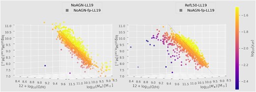
3D scatter plot in the M⋆–O/H–MH, tot space for the NoAGN (left-hand panel) and RefL50 (right-hand panel) simulations (see Table 1, for details), colour-coded with yeff. All quantities are calculated using similar apertures and definitions as in LL19. The grey surface represents the fitting plane (edge-on view) obtained for the NoAGN simulation. More viewing angles are available in the Supplementary Material.
For the sake of comparison with observational samples constituted by SF galaxies, we re-analysed the M⋆, gZgR corresponding to the RefL50 simulation (Fig. 11, right panel) for systems with sSFR > 10−11[yr−1]. Results are shown in Fig. 12. It is clear that very large deviations from the NoAGN-fp-LL19 (edge-on grey surface) are not expected for SF galaxies. These trends align with the notion that such deviations are primarily generated by galaxies that are more affected by AGN feedback, as extensively discussed in previous sections. Nevertheless, we would like to notice that, although host galaxies currently showing AGN activity are usually removed when studying metallicity scaling relations, AGN feedback might have occurred in cyclic episodes that affected the progenitors of observed galaxy populations. In eagle, AGN activity also evolves with time and all BHs are actively accreting gas some part of the time, giving place to the AGN phenomenon. In other words, although the accretion rate onto the BH could be low today, the BH activity could have been more significant in the past. This can be seen in Fig. 9, where it is clear that the BH accretion rates at z = 0 (|$\dot{M}_{\rm BH,accr \, (z=0)}$|) can be much lower than the median of this quantity along the galaxy lifetime (|$\langle \dot{M}_{\rm BH,accr \, (z)} \rangle$|). In the particular case of galaxies shown in Fig. 12, we find that, for |$\approx 50~{{\ \rm per\ cent}}$| of the sample, |$\dot{M}_{\rm BH,accr \, (z=0)}/\langle \dot{M}_{\rm BH,accr \, (z)} \rangle \lt 1$|.
![3D scatter plot in the M⋆–O/H–Mgas space for the RefL50 simulation. Only galaxies with sSFR > 10−11[yr−1] are plotted. The colour bar indicates the MBH/M⋆ of each galaxy. All quantities are calculated using similar apertures and definitions as in LL19. The grey surface represents the best-fitting plane (edge-on view) obtained for the NoAGN simulation. To explore other viewing angles, check the Supplementary Material.](https://oup.silverchair-cdn.com/oup/backfile/Content_public/Journal/mnras/528/4/10.1093_mnras_stae490/1/m_stae490fig12.jpeg?Expires=1750260772&Signature=Zju7hUZYWBUdMlE71jmLYr5PZbspeFM~XHQH-t1oGn2vsdzomdyLftRd1Oc0s7U45TbApQNTIYJOiHbXQWvgCpslTfb5367U8QU0CEVvpemTRQHO0sCu1bCo1TJJ2oSz3tYi65jgUXHp95ARcP9zf5OfyhDDpkCxZ3DorvMXOPgyxXVSet1df28hAjpeZcLVa7a7u6RZx6iFkngxg0PbjPrLI8mzUNTG-gi9SbVFBgyXXSMNyOEw9F~etxfmFqQP4LaRzzha0JITKbbjsHc8Z0FnVchla74kBrnpabB-qZFJbCs49~AkuarjeFercs6McpvjK7CAU7OvgDe0mE~c2w__&Key-Pair-Id=APKAIE5G5CRDK6RD3PGA)
3D scatter plot in the M⋆–O/H–Mgas space for the RefL50 simulation. Only galaxies with sSFR > 10−11[yr−1] are plotted. The colour bar indicates the MBH/M⋆ of each galaxy. All quantities are calculated using similar apertures and definitions as in LL19. The grey surface represents the best-fitting plane (edge-on view) obtained for the NoAGN simulation. To explore other viewing angles, check the Supplementary Material.
Finally, in Fig. 13, we analyse the LL19,observational sample in the 3D parameter space given by gas mass, stellar mass, and O/H.6 Encouragingly, the observed galaxy sample is located around our previously defined NoAGN-fp-LL19, which is shown as a yellow surface in the figure. The good agreement between observations and eagle simulations regarding the behaviour of effective yields has already been noted by LL19. The highest (lowest) observed yeff can be associated with galaxies above (below) the plane, with the residuals δ from such a plane, tracing variations in yeff. And, according to findings in this paper, the behaviour of yeff (and, hence, of δ) is significantly modulated by the joint accumulated effects of SN and AGN feedback. Although disentangling the impact of the latter processes could not be plausible in many cases, the location of galaxies with respect to the plane can provide some hints about their feedback histories, as we discuss in the next section.
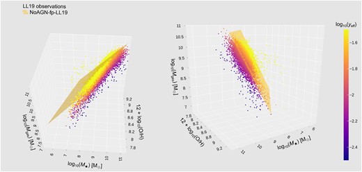
3D scatter plot in the M⋆–O/H–Mgas space for the LL19 observational data, colour-coded with yeff. The yellow surface represents the best-fitting plane obtained for the NoAGN simulation, when quantities are calculated using similar apertures and definitions as in LL19 (see the text for details). We encourage the reader to see the Supplementary Material for more viewing angles.
5.4 Connecting the features of the M⋆, gZgR to the plausible feedback histories of galaxies
Our findings suggest a close connection between feedback, yeff, and the location of galaxies in the 3D M⋆-O/H-Mgas parameter space, which could be useful for proposing feedback scenarios for real galaxy populations.
As extensively discussed, simulated galaxies that were not significantly affected by AGN feedback (MBH/M⋆ ≈ 0) are well represented by a plane in the aforementioned 3D space, with this plane located along a region of an almost constant high yeff. Interestingly, the existence of such a plane seems to be robust against the different variations that we implemented for defining our main properties (i.e. gas mass, stellar mass, and O/H), as explained in previous sections. But, our different definitions lead to moderate changes in the normalization and orientation of the plane (Table 2). In particular, when defining the properties of simulated galaxies according to those of SF galaxies in the Local Universe, galaxies in the latter sample are located around the plane derived from simulations.
Our findings so far suggest that the location of galaxies around such characteristic plane could provide clues about the feedback histories of real galaxies, as indicated below:
Galaxies that are well represented by the plane show an almost constant high yeff and nearly null residuals δ. Such galaxies are not expected to have been significantly affected by AGN feedback (MBH/M⋆ ≈ 0).
Considering the scatter obtained for the plane (e.g. ϵ in Table 2), galaxies with residuals δ below such characteristic value can be considered more affected by the accumulated effects of AGN feedback. Such galaxies are expected to display very high MBH/M⋆ and very low yeff, compared with the median population located closer to the plane.
For a reference AGN feedback efficiency, galaxies more strongly affected by SN feedback tend to lie slightly below the NoAGN-fp (δ ≲ 0) and do not reach very high yeff values. Thus, galaxies with the highest yeff (those above the plane) cannot be regarded as systems strongly affected by SN feedback.
For a reference AGN feedback efficiency but a weak SN feedback, we detect two different trends: (1) galaxies with higher MBH/M⋆ show lower yeff and negative distances to the plane (δ < 0); (2) galaxies with lower MBH/M⋆ have higher yeff and tend to be located above the NoAGN-fp (δ ≳ 0). Hence, galaxies with the highest yeff (those above the plane) can be associated with systems with both a weak SN feedback efficiency and a weak AGN feedback impact.
We note that we do not have information regarding BH masses for our observational sample. Future determination of these masses would be very useful to test the predictions of our simulations.
Finally, it is worth acknowledging that the comparison between simulations and observations could not be so straightforward. As discussed in De Rossi et al. (2017), the normalization of the observed M⋆ZgR is still a matter of discussion, with different observational works reporting a variety of results due to the use of distinct metallicity calibrators. In addition, uncertainties in the nucleosynthetic yields implemented in simulations can also affect the determination of absolute metallicity values. This issue regarding the calibration of absolute metallicities affects also the estimate of yeff (equation 2). In this context, the comparison of global metallicities and yeff between simulations and observations should be addressed with care.
6 SUMMARY AND CONCLUSIONS
We have analysed the effective yields (yeff) of galaxies in eagle cosmological hydrodynamical simulations that implement different SN and AGN feedback prescriptions: reference models calibrated against some observations (simulations RefL50 and RefL25); a model with weaker SN feedback (WeakFB simulation), and another with stronger SN feedback (StrongFB simulation); a simulation without BHs and, hence, without AGN feedback (NoAGN simulation); and a simulation which applies a higher gas temperature increment (ΔTAGN) associated with AGN feedback (AGNdT9 simulation), which drives a stronger AGN feedback impact according to previous works. In particular, we try to evaluate the role of SN and AGN accumulated feedback effects on the determination of yeff and the features of its associated scaling relations. For our main analysis, galaxy properties whose definitions involve gas (e.g. chemical abundances, gas fractions, and yeff) were derived from the SF gas-phase. But, we also explored the effects of using other plausible definitions. Our most relevant findings and conclusions can be summarized as follows:
In agreement with previous works, the reference model predicts an average positive (negative) slope for the yeff–Mbar relation (Fig. 1) at low |$M_{\rm bar} \lesssim 10^{10}~{\rm M}_{\odot }$| (high |$M_{\rm bar} \gtrsim 10^{10}~{\rm M}_{\odot }$|). An increase of ΔTAGN generates a decrease of such a slope at high masses but has a no significant impact for low-mass systems. Interestingly, similar effects are obtained when applying a weaker SN feedback efficiency, given that it fosters the formation of a significant number of galaxies with dominant BH (i.e. with high BH mass–stellar mass ratio, MBH/M⋆). On the other hand, no dominant BHs are formed in the case of a strong SN feedback scenario. In comparison with the reference model, a stronger SN feedback leads to an overall decrease of yeff at all masses and also predicts a positive slope for the yeff–Mbar for the whole simulation mass range.
To understand the origin of yeff behaviour, we analysed the feedback impact on the key galaxy properties involved in the yeff definition: gas-phase metallicity, stellar mass, and gas mass (Figs 2 and 3). AGN feedback seems to drive the simultaneous decrease of the SF gas fraction and metallicity of massive galaxies (which have more dominant BHs), which explains their lower yeff. On the other hand, a stronger SN feedback efficiency favours the decrease of metallicity at fixed SF gas fraction, also leading to lower yeff. In the case of a weak SN feedback efficiency, a more complex behaviour arises because of the formation of BHs in a significant number of galaxies along our whole mass range: as a consequence of AGN feedback, galaxies with dominant BH show lower O/H, lower SF gas fractions and, hence, lower yeff, while galaxies with low MBH/M⋆ tend to have higher metallicities at a given SF gas fraction and, thus, higher yeff.
We found a clear anticorrelation between yeff and the MBH/M⋆ for galaxies in all studied feedback models (Fig. 4): galaxies with |$M_{\rm BH}/M_\star \lesssim 10^{-3.5}$| show a higher and roughly constant yeff, while, for galaxies with |$M_{\rm BH}/M_\star \gtrsim 10^{-3.5}$|, yeff strongly decreases with MBH/M⋆.
We also studied the distribution of galaxies in the 3D parameter space defined by gas-phase metallicity, M⋆, and gas mass (M⋆, gZgR) for different SN and AGN feedback models (Figs 5 and 6). Interestingly, we found that, when AGN feedback is turned off, the M⋆, gZgR is well described by a plane (NoAGN-fp), which is locally situated along a surface of constant yeff. Such a plane can roughly describe the behaviour of galaxies with no dominant BH (low MBH/M⋆) in all simulations, regardless of the implemented feedback model. Orthogonal departures from the plane (δ) can be directly associated with variations in yeff (i.e. different yeff isosurfaces are crossed when moving away from the plane). Deviations from the plane that generates an increase of yeff are regarded as ‘positive’ (i.e. galaxies are considered to be above the plane) in this work, and ‘negative’ (i.e. galaxies are considered to be below the plane), otherwise.
Galaxies highly affected by the accumulated effects of AGN feedback (i.e. systems with high MBH/M⋆) show very low yeff and present large negative deviations from the NoAGN-fp (Figs 4 and 7). If galaxies are not significantly affected by AGN feedback (MBH/M⋆ ≈ 0), they are located close to the NoAGN-fp, having an almost constant high value of yeff.
For a reference AGN feedback efficiency, a strong SN feedback generates a moderate displacement of the bulk galaxy population downward the NoAGN-fp, with such galaxies showing intermediate yeff values. For a reference AGN feedback efficiency but a weak SN feedback, we detect two different regimes: (1) galaxies with higher MBH/M⋆ show lower yeff and negative deviations from the plane; (2) galaxies with lower MBH/M⋆ have higher yeff and tend to be located above the NoAGN-fp (Figs 4 and 7).
A deeper analysis suggests that systems with larger negative δ present higher MBH/M⋆ as a consequence of their more significant amount of mass accreted via galaxy mergers (Fig. 8). This is because galaxy mergers tend to boost the gas accretion rate of the BH and also can drive BH mergers. The present and past average BH accretion rates of galaxies with higher MBH/M⋆ are also higher, indicating that such systems have been more significantly affected by AGN feedback during their evolution (Fig. 9).
Feedback-driven gas heating seems to be the main process responsible for larger yeff negative variations and higher deviations down the NoAGN-fp. Gas heating foster the transition from the SF to the NSF gas phase, affecting all our quantities derived from SF gas. If re-estimating these galaxy properties using the total gas component (including SF and NSF gas), almost the whole galaxy population in all studied simulations is located around a new plane in the 3D space given by gas-phase metallicity, M⋆, and gas mass (Fig. 10). The scatter around this plane is lower and no significant negative deviations from it are obtained.
The M⋆, gZgR of observed galaxies in the Local Universe also seems to be located around a plane, with the highest (lowest) effective yields associated with galaxies above (below) the plane. When we re-calculate our simulated quantities mimicking the observational definitions, the observed and simulated trends show very good agreement. In particular, the new plane derived from the NoAGN model (NoAGN-fp-LL19, Fig. 11) using such quantities represents again a surface of constant yeff and, encouragingly, this plane can characterize well the behaviour of observed galaxies with similar yeff (Fig. 13). In addition, if restricting our simulated galaxy sample to systems with sSFR > 10−11[yr−1] as in observations of SF galaxies, large negative δ are not obtained (Fig. 12).
To sum up, according to the findings in this paper, the evolution of yeff (and, hence, of δ) is significantly affected by the joint accumulated effects of SN and AGN feedback. Thus, the determination of yeff (or, equivalently, δ) and its associated scaling relations could provide relevant hints regarding the different feedback histories of real galaxy populations. Nevertheless, as discussed, caution should be taken when estimating the quantities involved in the definition of yeff, for a correct interpretation of observational data. In a forthcoming article, we will extend this study, addressing the effects of feedback on yeff at z > 0 (for preliminary results, see Zerbo et al. 2022).
ACKNOWLEDGEMENTS
We thank the reviewer for the constructive suggestions and comments that helped improve this paper. MCZ thanks Asociación Argentina de Astronomía for having been awarded with a grant, which partially supported this project. We thank Rodrigo Flores-Freitas for his useful help with some technical details regarding the preparation of the Supplementary Material. SAC acknowledges funding from CONICET (PIP-2876), Agencia Nacional de Promoción de la Investigación, el Desarrollo Tecnológico y la Innovación (Agencia I+D+i, PICT-2018-3743), and the Universidad Nacional de La Plata (G11-150), Argentina. We acknowledge support from PICT-2021-GRF-TI-00290 of Agencia I+D+i (Argentina). We acknowledge the Virgo Consortium for making their simulation data available. The eagle simulations were performed using the DiRAC-2 facility at Durham, managed by the ICC, and the PRACE facility Curie based in France at TGCC, CEA, Bruyères-le-Châtel. This work used the DiRAC@Durham facility managed by the Institute for Computational Cosmology on behalf of the STFC DiRAC HPC Facility (www.dirac.ac.uk). The equipment was funded by BEIS capital funding via STFC capital grants ST/P002293/1, ST/R002371/1, and ST/S002502/1, Durham University, and STFC operations grant ST/R000832/1. DiRAC is part of the National e-Infrastructure.
DATA AVAILABILITY
The eagle simulations are publicly available. Both halo/galaxy catalogues and particle data can be accessed and downloaded at www.icc.dur.ac.uk/Eagle/ (Crain et al. 2015; Schaye et al. 2015; McAlpine et al. 2016). To create the results shown in this publication, Python libraries were used (astropy, numpy, scipy, pyplot, and h5py), including the publicly available read_eagle module (https://github.com/jchelly/read_eagle, The EAGLE team 2017). Additional data and code directly related to this work are available on reasonable request from the corresponding author.
Footnotes
We note, however, that the exact normalization and shape of the M⋆ZgR are still debated. Different observational methods for inferring the key galaxy properties yield significantly different answers (Telford et al. 2016) and, hence, the comparison between simulations and observations is not straightforward.
The main branch of the merger tree is defined as the one with the largest stellar mass summed across all earlier simulation outputs, see McAlpine et al. (2016) for more details.
We remind that caution should be taken when studying the simulated BH accretion rates since the time sampling may not accurately capture their high temporal variability (see Section 2.1.3).
We acknowledge, however, that there are still many controversies regarding the exact value of the slope and zero-point of the M⋆ZgR. The use of different selection criteria and methods for the estimates of stellar masses and metallicities affects the comparison between different observational data.
The reader is refereed to LL19 for a description of the procedures used for deriving galaxy quantities in observations.
