


ABSTRACT
We present and analyse the results of quasi-simultaneous spectroscopic, photometric, and polarimetric observations of hyperbolic comet C/2013 X1 (PANSTARRS) obtained at the 6-m Big Telescope Alt-azimuth (BTA) telescope Special Astrophysical Observatory (SAO) and 2.6-m Shajn telescope Crimean Astrophysical Observatory (CrAO). A wide fan-shaped structure and a weak tail were detected in the comet. The mean V − R colour of the coma was estimated to be neutral compared to the solar value. The Afρ parameter, a proxy to the dust production in the comet, was about 1672 ± 21 cm in the R band. Emissions of the CN, C2, C3, and NH2 molecules were identified in the cometary spectrum, which covers the wavelength range 3800 – 7100 Å. When the comet was at a distance of 2.66 au from the Sun, the minimum degree of polarization of about −1.5 per cent was detected in the near-nucleus region of the coma, in the range up to about 10 000 km from the optocentre. Further, polarization gradually increased (in absolute value) with distance from the nucleus, reaching −6.5 per cent at about 50 000 km. To reproduce the observed values of linear polarization and the phase-angle dependence of polarization for long-period comets, we used the Sh-matrix method with conjugated Gaussian random particles as light scatters, and the chemical composition of dust particles in the coma of 74 per cent amorphous carbon, 25 per cent of Mg-rich silicates, and 1 per cent of water ice.
1 INTRODUCTION
Dynamically new comets, coming from the Oort Cloud at their first passage close to the Sun, are particularly important because their matter is supposed to preserve primordial material not processed by solar radiation. It is believed that short-period comets with orbital periods of Porb < 200 yr contain well-processed materials on their surfaces. Long-period comets are between these two extremes. They could come into the inner part of the Solar system previously, but their orbital periods are comparatively longer (Porb > 200 yr). Therefore, it is possible to investigate not only the primordial matter of our planetary system but also its current state. Moreover, studying long-period comets is also a key element in understanding dust’s evolution from earlier times to nowadays.
Comet C/2013 X1 (PANSTARRS), hereinafter C/2013 X1, was discovered on 2013 December 4 by the Panoramic Survey Telescope and Rapid Response System (Pan-STARRS 1) located at Haleakala Observatory in Hawaii (Bolin et al. 2013), when it was at 8.9 au from the Sun and its magnitude was 20.2 mag. This is a hyperbolic comet with an orbital eccentricity of 1.001 026 ± 0.000 002 and an inclination of 163.23°.1 Manzini et al. (2016) assumed that it could be a dynamically old comet. At the same time, Combi et al. (2018) classified the comet as a young long-period comet in the Oort sense (see A’Hearn et al. 1995). Comet C/2013 X1 reached a perihelion distance of 1.31424 au on 2016 April 20.
Since comet C/2013 X1 was expected to be bright near perihelion, it has been actively studied since its discovery. Several groups carried out monitoring observations to investigate the evolution of its activity. Sárneczky et al. (2016) performed observations during several nights in 2013–2014 and revealed an increase in the dust production rate almost three times. They also noticed the fuzzy appearance of the coma during observations and the beginning of tail formation. Manzini et al. (2016) and Trigo-Rodríguez et al. (2016) performed observations in the same time period. The former group of the authors provided a detailed analysis of the coma morphology. They reported a faint dust tail and wide triangular fan which was fairly stable during four months of observations. Trigo-Rodríguez et al. (2016) provided multiband photometry of the comet and detected the outburst on 2016 January 2.79. Another pre-perihelion outburst was reported by Combi et al. (2018) based on the water production rate during the pre- and post-perihelion passage of the comet. After perihelion, the water production rate in the comet gradually decreased as the heliocentric distance increased. High-resolution spectra of comet C/2013 X1 were obtained in the near-infrared (IR) spectral range 0.9–2.5 μm, and a detailed study of the red CN system in the 1.1 μm range, as well as many other emission lines, was carried out (Faggi et al. 2016). Post-perihelion observations of comet C/2013 X1 also showed a slightly lower level of dust production rate than that observed in 2013–2014 (Moulane et al. 2017). Based on mid-IR 6.0 µm ≤ λ ≤ 40 μm spectrophotometric observations, Woodward et al. (2021) determined the composition of the dust in the coma, which was dominated by dark dust particles (modelled as amorphous carbon) with a carbon-to-silicate ratio of 7.781 ± 6.091. Wooden et al. (2021) have concluded that this comet is carbon-rich. A high-resolution spectrum and HCN image of comet C/2013 X1 were acquired in the submillimetre range on 2016 June 10 (Primiani et al. 2016). The detected HCN molecule may be one of the parent molecules of the CN radical identified in the optical spectrum of this comet. The authors noted that the HCN emission peaked around the nucleus but with a clear extension towards the antisolar direction.
This work presents the results of quasi-simultaneous spectroscopic, photometric, and polarimetric observations of comet C/2013 X1 performed with the 6-m Big Telescope Alt-azimuth (BTA) telescope Special Astrophysical Observatory (SAO), as well as polarimetric observations with the 2.6-m Shajn telescope Crimean Astrophysical Observatory (CrAO), before its perihelion passage. These observations and the data reduction techniques are described in Section 2. The results of spectroscopy and photometry of the comet are given in Section 3. The Sh-matrix model with conjugated random Gaussian particles used to interpret the polarimetric data is presented in Section 4. Our findings are summarized in conclusions.
2 OBSERVATIONS AND DATA REDUCTION
The pre-perihelion observations of comet C/2013 X1 were carried out at the 6-m telescope BTA of the SAO on 2015 November 4 and at the 2.6-m Shajn telescope of the CrAO on 2015 November 13 and 2016 January 13. The multimode focal reducer SCORPIO-22 (Afanasiev & Moiseev 2011; Afanasiev & Amirkhanyan 2012) attached to the prime focus of the 6-m telescope was used. On 2015 November 4, observations of the comet were carried out in the packet mode which allowed us to make a sequence of exposures to obtain direct CCD images, spectra with a long slit, and imaging linear polarimetry. We used the CCD chip E2V-42-90 with 4612 × 2048 square pixels of 13.5 μm corresponding to 0.18 arcsec on the sky plane without binning.
Image processing, including bias subtraction, flat-field correction, and other specified procedures, was performed via a standard algorithm for each observation mode using software created for the SCORPIO-2 instrument (Afanasiev & Moiseev 2011; Afanasiev & Amirkhanyan 2012). The detailed data processing is described in Ivanova et al. (2019).
For observations at the 2.6-m telescope, we used a one-channel photoelectric photometer-polarimeter. The comet was observed in the WR filter (spectral band 5500–7500 Å) with a 30 arcsec diaphragm centred on the comet photometric centre. The weather conditions were bad due to being partly cloudy. However, the use of the fast rotating (∼33 Hz) quarter-waveplate (λ/4) and the synchronous detection method used makes it possible to measure the polarization under poor conditions. The basic version of the polarimeter, the reduction of polarimetric data, and the practical aspects of linear polarization measurements are described by Shakhovskoj & Efimov (1972), and subsequent modifications by Kolesnikov et al. (2016).
2.1 Spectroscopy
We derived the spectra of comet C/2013 X1 with a long slit using the transparent grism VPHG1200|$@$|540 as a disperser in the spectroscopic mode of the SCORPIO-2. The slit of 6.1 arcmin × 1.0 arcsec was centred on the optocentre of the coma, which is assumed to be the position of the cometary nucleus in the plane of the sky, and oriented along the velocity vector of the comet. The obtained spectra cover the wavelength range 3600–7070 Å and have a dispersion of 0.87 Å px−1. The spectral resolution of spectra, defined by slit width, is 5.2 Å. We applied 1 × 2 binning to increase the signal-to-noise ratio. The wavelength calibration was made using the spectrum of the He–Ne–Ar calibration lamp. We used a smoothed spectrum of an incandescent lamp to provide flat-field corrections to the spectral data. To convert the observed cometary count rates into absolute fluxes, we used the spectra of the standard star BD + 25d4655 (Oke 1990), which was observed on the same night. We used the measurements of the spectral atmospheric transparency at the Special Astronomical Observatory taken from (Kartasheva & Chunakova 1978). During spectroscopic observations, the seeing was 1.2 arcsec. Some parts of the CN and C2 emission bands cover the entire height of the slit. Therefore, the spectrum of the night sky was determined by measuring it in each column across the dispersion in zones free from cometary emissions, followed by a polynomial fit to the part of the column with cometary radiation. Then, this spectrum was used for a polynomial approximation in those narrow zones along the dispersion where cometary emissions are present. Thus, we constructed the full spectrum of the night sky, which was subtracted from the observed spectrum of the comet.
2.2 Photometry
The direct images of comet C/2013 X1 are obtained with the broad-band g-sdss filter (the central wavelength λ0 and full width at half-maximum are λ4650/1300 Å) at the 6-m telescope. The field of view of the image is 6.1 arcmin × 6.1 arcmin. In this case, we applied 2 × 2 binning which corresponds to the scale of 461 km px−1. Photometric calibration of comet images was made using the standard stars over the field of view. To recalculate the intensities into the fluxes, we used catalogue UCAC4 (Zacharias et al. 2013) with an accuracy of 0.05–0.1 mag. Since the comet and standard stars were observed at almost the same zenith angle, we assumed a negligible airmass discrepancy. The night sky light contribution was extracted using a standard idl sky-subtraction routine.
2.3 Polarimetry
The images of the comet in polarized light were taken through the broad-band Johnson–Cousins R filter (λ6400/1580 Å) using the 6-m telescope with the SCORPIO-2 in the polarimetric mode. For linear polarization measurements of the comet, we used the dichroic polarization analyser (called POLAROID) which was positioned in three fixed positions at angles +60°, 0°, and −60° (Afanasiev & Amirkhanyan 2012). Using the intensities measured at these angles, we calculated the Stokes parameters q and u, normalized to the total intensity, at each pixel of the image. To determine the instrumental polarization and the correction for the zero-point of the position angle of the polarization plane, we observed the polarized and non-polarized standard stars with well-known interstellar polarization taken from the lists of Hsu & Breger (1982), Schmidt, Elston & Lupie (1992), and Heiles (2000). Typically, the instrumental polarization was less than 0.1 per cent. The error in the measured polarization of the comet is about 0.12 per cent in the central part of the image where the comet is located.
As a rule, the instrumental polarization of the photometer–polarimeter at the 2.6-m telescope was less than 0.2 per cent. Errors in the degree of linear polarization of the comet varied from 0.14 per cent on 2015 November 13 to 0.76 per cent on 2016 January 13, depending on the signal accumulation time and the weather conditions.
More details about the viewing geometry and observation log of comet C/2013 X1 are given in Table 1. Date of observations, telescope, observation mode, filter or grid, heliocentric (r) and geocentric (Δ) distances, phase angle (α), position angle of the extended Sun-to-target radius vector (ψ), the total exposure time (Texp), and the number of observation cycles (N) are given in the table. Photometric, spectral, and imaging polarimetry modes are designated ImPho, Spectral, and ImPol, respectively, and photoelectric polarimetry is Pol.
Observation log of comet C/2013 X1 (PANSTARRS).
| Date (ut) | Telescope | Mode | Filter/grid | r (au) | Δ (au) | α (°) | ψ (°) | Texp (s) | N |
|---|---|---|---|---|---|---|---|---|---|
| 2015 Nov 04 | 6-m | Spectral | VPHG1200|$@$|540 | 2.658 | 1.781 | 12.26 | 216.12 | 120 | 3 |
| ImPol | R | 30 | 90 | ||||||
| ImPho | g-sdss | 30 | 5 | ||||||
| 2015 Nov 13 | 2.6-m | Pol | WR | 2.561 | 1.640 | 10.08 | 179.73 | 128 | 48 |
| 2016 Jan 13 | 2.6-m | Pol | WR | 1.930 | 1.981 | 29.11 | 60.24 | 128 | 3a |
The bad weather conditions.
3 RESULTS
3.1 Spectroscopy
Using the long-slit spectrum of comet C/2013 X1 allowed us to study spectral energy distribution within the 3800–7100 Å wavelength range. To isolate the emission spectrum of the comet, the cometary continuum must be subtracted from the observed cometary spectrum. For this purpose, we convolved a high-resolution spectrum of the Sun (Neckel & Labs 1984) with an appropriate instrumental profile to the cometary spectrum resolution and normalized to the flux from the comet using a polynomial fit. In this way, the reddening effect was also taken into account. The emission spectra of the comet were obtained by subtracting the calculated continuum from the observed spectrum. The observed spectrum of the comet with the superimposed continuum, as well as the emission spectra, are displayed in Fig. 1. Note that the detector we used has lower sensitivity in the blue region, therefore the blue region of the spectrum is noisier.

The spectrum of comet C/2013 X1 (PANSTARRS): the observed cometary spectrum (black curve) and continuum (red curve) are presented in the top panel, and the emission spectrum with identified molecular features is shown in the bottom one.
Despite the relatively large heliocentric distance of 2.66 au, 54 molecular emissions were identified in the spectrum, the strongest of which belong to the CN, C2, C3, and NH2 molecules. Ganesh et al. (2018) obtained a similar emission spectrum on 2015 November 30, when the comet was at a heliocentric distance of 2.38 au.
The energy distribution in the continuum spectrum of the comet is characterized by the so-called reddening effect, i.e. the change in the light scattering efficiency with increasing the wavelength: |$S(\lambda) = \frac{F_{\mathrm{ c}}(\lambda)}{F_{\mathrm{ Sun}}(\lambda)} ,$|, where Fc(λ) and FSun(λ) are the radiation fluxes from the comet and the Sun, respectively. To obtain FSun, we convolved the cometary continuum with the transmission curve of the cometary continuum filters (Osborn et al. 1990; Farnham, Schleicher & A’Hearn 2000). For analysis of the dust component of the cometary coma, we computed the normalized spectral gradient of the reflectivity S′ within two wavelengths ranges λ1 and λ2, using the following equation (A’Hearn et al. 1984):
where λ1 < λ2. We obtained the normalized reflectivity gradients S′ = (13 ± 3) per cent per 1000 Å for the spectral range between the BC (blue continuum, λ4450/67 Å) and RC (red continuum, λ6840/90 Å) cometary bands in the continuum (Osborn et al. 1990; Farnham, Schleicher & A’Hearn 2000). The derived value of the spectral gradient demonstrates the general trend of the reflectivity noted by Jewitt & Meech (1986): it decreases systematically with increasing wavelength. On the whole, our results can be considered typical of long-period comets. Storrs, Cochran & Barker (1992) obtained the value of the reflectivity gradient of 15–37 per cent per 1000 Å for the 4400–5600 Å spectral region based on observations of 18 ecliptic comets. Kulyk et al. (2018) studied another sample of long-period comets and obtained mean gradients within this group: 14 ± 2 per cent per 1000 Å and 3 ± 2 per cent per 1000 Å for the B–V and V–R spectral ranges, however, the gradients vary within these ranges from 6 to 22 and from −3 to 24 per cent per 1000 Å, respectively.
Using the spectral data, we estimated the dust production rate in comet C/2013 X1. For this, we used the expression from A’Hearn et al. (1984) for the calculation of the Afρ parameter (in cm), which is a proxy of dust production rate:
where A is the mean particle albedo at a phase angle α, f is the filling factor of the coma, Δ is the geocentric distance of the comet (in cm), r is the heliocentric distance of the comet expressed in au, ρ is the linear radius of the aperture at the comet’s position (in cm). The radiation fluxes of the cometary continuum, Fc, and the Sun, FSun are taken within an appropriate filter. According to A’Hearn et al. (1984), a circular aperture is supposed to be used to calculate Afρ. However, in the case of spectral investigations, a rectangular slit is used as a diaphragm. Therefore, we calculated the effective radius of the circular aperture based on the slit area. The quantities of Afρ calculated in an aperture with an effective radius of about 13 850 km for three spectral bands BC, GC, and RC used in comet studies are presented in Table 2, which shows the numerical values with their errors. Here, we also added the A(0°)fρ values corrected for the phase-angle effect according to Schleicher, Millis & Birch (1998), that is, the values of Afρ normalized to the phase angle 0°. Moulane et al. (2017) computed the production rate of dust by comet C/2013 X1 in the BC filter based on observations made seven months after our ones, on 2016 June 7 – 27. Using photometric data, the authors obtained higher values of the Afρ parameter, from 857 to 1260 cm.
The dust production rate obtained from the spectral and photometric observations of comet C/2013 X1 (PANSTARRS) on 2015 November 4 at the heliocentric distance of 2.658 au.
| Filter (λc/Δλ, Å) | Afρ (cm) | A(0°)fρ (cm) |
|---|---|---|
| BC (4429/36) | 237 ± 11 | 368 |
| GC (5260/56) | 279 ± 12 | 433 |
| RC (6835/83) | 1127 ± 25 | 1749 |
| R (6400/1580) | 1672 ± 21 | 2598 |
| g-sdss (4650/1300)a | 1510 ± 26 | 2346 |
| Filter (λc/Δλ, Å) | Afρ (cm) | A(0°)fρ (cm) |
|---|---|---|
| BC (4429/36) | 237 ± 11 | 368 |
| GC (5260/56) | 279 ± 12 | 433 |
| RC (6835/83) | 1127 ± 25 | 1749 |
| R (6400/1580) | 1672 ± 21 | 2598 |
| g-sdss (4650/1300)a | 1510 ± 26 | 2346 |
From photometry.
To determine the production rates of gas molecules, we used the classic Haser model (Haser 1957) to the observed column densities. The values of gas production rate are strongly dependent on the input parameters, such as the fluorescence efficiency of the molecule (g-factor) and parent and daughter molecules scale lengths (lp and lp, respectively). The values of these parameters were taken from Langland-Shula & Smith (2011) and are given in Table 3. It should be noted that we recalculated these parameters to the observed heliocentric distance of the comet according to r-n, where the power-law index n is indicated in the table.
Model parameters recalculated to the heliocentric distance at which the spectrum of comet C/2013 X1 (PANSTARRS) was observed.
| Molecule | g-factor | lp | ld | n |
|---|---|---|---|---|
| (watt mol−1) | (104 km) | (105 km) | ||
| CN (Δv = 0) | 5.22 × 10⁻²¹ | 9.21 | 14.87 | 2 |
| C3 (Δv = 0) | 1.41 × 10⁻²⁰ | 1.98 | 1.91 | 2 |
| C2 (Δv = 0) | 6.36 × 10⁻²¹ | 15.58 | 4.67 | 2 |
| Molecule | g-factor | lp | ld | n |
|---|---|---|---|---|
| (watt mol−1) | (104 km) | (105 km) | ||
| CN (Δv = 0) | 5.22 × 10⁻²¹ | 9.21 | 14.87 | 2 |
| C3 (Δv = 0) | 1.41 × 10⁻²⁰ | 1.98 | 1.91 | 2 |
| C2 (Δv = 0) | 6.36 × 10⁻²¹ | 15.58 | 4.67 | 2 |
The fluorescence efficiency for the CN molecule depends on the heliocentric distance as well as the heliocentric velocity of the comet. Schleicher (2010) tabulated the g-factor values for various heliocentric distances and velocities, which we used in our calculations. For the gas outflow velocity, we adopted the value 1 km s−1 used in most of such calculations (e.g. Langland-Shula & Smith 2011). The Haser model assumes a spherically symmetric gas outflow with a constant velocity, and this means that the model expression for the calculation of the production rate of gas molecules is valid for the circular aperture. Since the cometary spectra are derived with a long slit, we need to convert the fluxes obtained with a long-slit aperture into an equivalent circular aperture. Therefore, for the correct application of the Haser model formula, we included in the measured data a coefficient equal to the ratio of the areas of the used aperture and the spectrograph slit located within that aperture. We used the aperture with a radius of 10.72 arcsec or 13 847 km. Using all the necessary parameters and corrections, we calculated the production rates of the CN, C2, and C3 molecules in comet C/2013 X1. The results are presented in Table 4. In general, the gas production rates in the comet are in good agreement with the literature data obtained for long-period comets at similar heliocentric distances. Using the observations within narrow-band cometary filters, Moulane et al. (2017) obtained the production rates of CN, C2, and C3 molecules in comet C/2013 X1 after its perihelion passage on 2016 June 07 – 27. The mean values of the gas production rates during this observational period are given in the table. As one can see, the data of Moulane et al. (2017) are lower than what we obtained. The main reason for this discrepancy may be that we observed the comet 168 d before perihelion, whereas Moulane et al. (2017) observed 48–68 d after perihelion.
Gas production rates in comet C/2013 X1 (PANSTARRS).
| Date (ut) | r (au) | Q (mol s−1) | Reference | ||||
|---|---|---|---|---|---|---|---|
| CN | C3 | C2 | log[Q(C3)/Q(CN)] | log[Q(C2)/Q(CN)] | |||
| × 1026 | × 1025 | × 1026 | |||||
| 2015 Nov 4 | 2.658 | 5.01 ± 0.24 | 3.98 ± 0.25 | 3.16 ± 0.07 | −1.10 ± 0.05 | −0.20 ± 0.03 | This work |
| 2016 June 7–27 | 1.49–1.65 | 1.20 | 2.48 | 1.74 | −0.68 | 0.16 | Moulane et al. (2017) |
According to A’Hearn et al. (1995), the typical comets show the ratio log[Q(C2)/Q(CN)] ≥ −0.18 with a mean value of this ratio 0.06 ± 0.10 and limits between −0.09 and 0.29. At the same time, the carbon-depleted comets have the ratio log[Q(C2)/Q(CN)] < −0.18, a mean value in the log of −0.61 ± 0.35 and limits from −1.22 to −0.21. Cochran, Barker & Gray (2012) used for the analysis of the spectral data set of 110 comets and also found two classes of comets: typical and carbon-chain depleted comets, requiring C2 and C3 to both be depleted. These authors defined the depleted comet as comet showing log[Q(C3)/Q(CN)] ≤ −0.86 and log[Q(C2)/Q(CN)] ≤ 0.02. According to the data base of comets given in Schleicher (2008) (see also Moulane et al. 2023), the mean relative molecular abundances for depleted comets are log[Q(C2)/Q(CN)] = −0.61 ± 0.35 and log[Q(C3)/Q(CN)] = −1.49 ± 0.14, while for typical comets log[Q(C2)/Q(CN)] = 0.10 ± 0.10 and log[Q(C3)/Q(CN)] = −0.57 ± 0.11. Fink (2009) reanalysed the spectral data for 50 comets with measurable emissions observed during 1985 – 2004 and found that after transformation of the ratios to A’Hearn et al. (1995) scale lengths, 35 comets of typical composition showed the mean value of log[Q(C2)/Q(CN)] = 0.08 ± 0.19 which is close to the A’Hearn et al. (1995) value, while 11 depleted comets had the average value log[Q(C2)/Q(CN)] = −0.53 ± 0.18. The author classified comets with the ratio log[Q(C2)/Q(CN)] < −0.29 [after converting the ratios to A’Hearn et al. (1995) scale lengths] as C2-depleted comets. According to this definition, the dynamical family of 21 long-period comets is not C2-depleted and appears to show enhanced C2/CN ratios.
Langland-Shula & Smith (2011) analysed the variations of log[Q(C2)/Q(CN)] and log[Q(C3)/Q(CN)] ratios with heliocentric distance using a set of comets belonging to different dynamical groups. The two carbon-chain species C2 and C3 showed very different behaviour than CN. Corresponding to the values found by A’Hearn et al. (1995) and Cochran et al. (2012), the log[Q(C3)/Q(CN)] ratio remained almost unchanged with heliocentric distance, while the log[Q(C2)/Q(CN)] ratio increased sharply as a comet approached the Sun. For a sample of only long-period comets, the authors obtained average values of the ratios log[Q(C3)/Q(CN)] = −0.8 ± 0.1 and log[Q(C2)/Q(CN)] = −0.1 ± 0.1.
In addition to observations of comet C/2013 X1 in the optical region, it was observed in the IR spectral range at the SOFIA Observatory (Wooden et al. 2021; Woodward et al. 2021). Derived from these observations, the elemental C/Si ratio is within a factor of 2.5 less than interstellar medium and solar C/Si ratios and is much higher than in carbonaceous chondrites; thus, indicating that comet C/2013 X1 should be carbon-rich.
From this brief analysis, the question of whether long-period comet C/2013 X1 belongs to the class of carbon-deficient comets or typical comets is unclear. Indeed, from our observations it follows that comet C/2013 X1 has the ratios log[Q(C3)/Q(CN)] = −1.10 and log[Q(C2)/Q(CN)] = −0.20, while Moulane et al. (2017) obtained, respectively, −0.68 and 0.16 (see Table 4). According to the criteria of A’Hearn et al. (1995) and Cochran et al. (2012), our data indicate that comet C/2013 X1 could be classified as a carbon-depleted comet, whereas the data of Moulane et al. (2017) lead to the opposite conclusion. However, according to the most complete data base of comets given in (Schleicher 2008), the mean relative molecular abundances for depleted comets are log[Q(C2)/Q(CN)] = −0.61 ± 0.35 and log[Q(C3)/Q(CN) = −1.49 ± 0.14. Comparing our results with those derived by Langland-Shula & Smith (2011), we found that comet C/2013 X1 has a higher value of log[Q(C2)/Q(CN)] and a lower value of log[Q(C3)/Q(CN)] compared to the corresponding best-fitting power-law relations (see fig. 22 in Langland-Shula & Smith 2011), although the production ratios for comet C/2013 X1 are slightly lower compared to those of the studied long-period comets. In addition, Fink (2009) concluded that there are no C2-depleted comets among long-period comets. Thus, given all the above data on the molecular carbon content of comets and the uncertainty in our ratios of C2 and C3 relative to CN, we conclude that comet C/2013 X1 most likely has a typical molecular composition.
3.2 Photometry
3.2.1 Morphology
The intensity map of comet C/2013 X1 was created by summation of coaligned individual images taken with a short exposure (see Table 1) to achieve good signal-to-noise ratios to determine the brightness distribution over the coma and its morphology, colour, and dust production rate. The resulting intensity map in the g-sdss filter is presented in Fig. 2a. As one can see, the observed coma demonstrated a very asymmetrical shape. To reveal the low-contrast structures in the inner coma of comet C/2013 X1, we applied enhancement techniques to the stacked image obtained and to each individual image of the comet for comparison to avoid false structures. For this procedure, we have used such digital filters as a rotational gradient method (Larson & Sekanina 1984) and division by averaged azimuthal profile (Samarasinha & Larson 2014) (Fig. 2b, c). After these enhancement procedures, we revealed unusual structures in the coma. The processed image in Fig. 2b shows the presence of a fan-shaped structure of the triangular shape located at position angle PA = 17°, which expands towards the Sun, while a faint, tail-like feature is seen in the opposite direction, PA = 225°. The image taken by Manzini et al. (2016) on the same night, 2015 November 4, also shows these structures, confirming the correctness of our findings. The fan structure remained quite stable during four months of observations by Manzini et al. (2016). According to these authors, the triangular shape of the fan is the result of a continuous outflow of dust from a single active source located at the latitude of about 60° on the surface of the cometary nucleus, the spin axis of which was placed near the sky plane. A detailed analysis of the evolution of morphology will be a topic of forthcoming research.
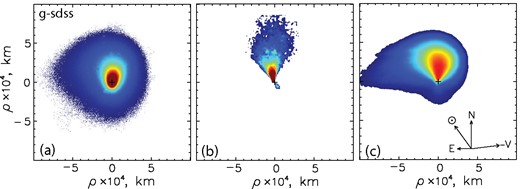
Stacked average image of comet C/2013 X1 (PANSTARRS) in the g-sdss filter taken with the 6-m BTA telescope on 2015 November 4 at r = 2.66 au (a); (b) is the image of the comet processed by a rotational gradient filter (Larson & Sekanina 1984); (c) is the image to which a division by 1/ρ profile was applied (Samarasinha & Larson 2014). The cross marks the position of the cometary nucleus. The arrows show the direction towards the Sun (⊙), the north (N), and east directions (E), and the negative heliocentric velocity vector (−V) of the comet as seen in the observer’s plane of the sky. The negative distance is in the solar direction, and the positive distance is in the antisolar direction.
3.2.2 Dust colour
To determine the dust colour using the broad-band filter for observations, we estimated the gas contribution to these filters from the spectral data as fluxes ratio of the emission spectrum to the observed one within the same filter. In the R and g-sdss bands, the gas contribution is approximately 3.8 and 8 per cent, respectively. The photometric observations of comet C/2013 X1 were performed with the broad-band g-sdss filter. To obtain the comet magnitude in the Johnson–Cousins V photometric system, we recalculated our measurements in the g-sdss filter using transformation equations from Lupton et al. (2005). The image in the R band was created from polarimetric observations performed in this filter. The result of our calculations is presented in Fig. 3a, which displays the distribution of the V − R colour over the coma of comet C/2013 X1. As one can see, there are variations in the dust colour along the fan from slightly red in the near-nucleus area to blue in the outer regions. The mean V − R colour over the coma of comet C/2013 X1 measured within the aperture with a radius of 10.7 arcsec (13 820 km) is (0.35 ± 0.04) mag which corresponds, within the measurement errors, to a neutral colour of the cometary dust compared to the Sun value of 0.39 mag (Willmer 2018). Based on three months of monitoring photometric observations carried out from 2015 November 18 to 2016 January 7, Trigo-Rodríguez et al. (2016) obtained a colour index V − R = (0.44 ± 0.05) mag determined within a 10 arcsec aperture. V − R colours measured in the near-nucleus coma of comet C/2013 X1 are neutral compared to the dust colour in other long-period comets at larger heliocentric distances (e.g. Mazzotta Epifani et al. 2010, 2014; Ivanova et al. 2015; Kulyk et al. 2018). For example, in hyperbolic comet C/2009 P1 (Garradd), dust colour near the nucleus is (0.39 ± 0.13) mag at r = 2.48 au (Mazzotta Epifani et al. 2016). Assuming that comet C/2013 X1 has the typical composition of dust (see Section 4.2 and Woodward et al. 2021), then neutral colour implies that the particle sizes should be on average of the order of the wavelength since the scattering cross-section for particles that are much larger and much smaller than the wavelength depends strongly on the size parameter, and therefore on the wavelength.
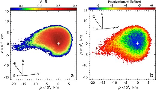
Distribution of the V − R colour (a) and polarization degree (b) over the coma of comet C/2013 X1 (PANSARRS) obtained on 2015 November 4. The cross marks the position of the cometary nucleus. The arrows show the same directions as in Fig. 2.
3.2.3 The dust production rate
To estimate the production rate of dust in comet 2013 X1 from the photometric data obtained in the g-sdss band, we used the Afρ (in cm) parameter, which is calculated according to the following expression (A’Hearn et al. 1984):
where A, f, r, and Δ are the same parameters mentioned in equation (2), and mc and mSun are the apparent magnitudes of the comet and the Sun, respectively, obtained within the aperture radius of ρ. In our calculations, we used apparent solar magnitudes in appropriate filters taken from Willmer (2018). The parameter Afρ depends on the phase angle of the comet, so we applied the phase-angle correction proposed by Schleicher, Millis & Birch (1998) for comet Halley to normalize Afρ to a 0° phase angle. The Afρ value calculated for comet C/2013 X1 within the aperture with a radius of 13 820 km and corrected for the phase-angle effect (denoted as A(0°)fρ) are given in Table 2. Sárneczky et al. (2016) also observed comet C/2013 X1 through the R filter in the inbound leg of the orbit for five nights, from 2013 December 27 to 2014 October 28. The authors determined the dust production in the comet and found a monotonic increase in Afρ from 451 to 1400 cm at heliocentric distances from 8.71 to 6.26 au. To compare our result with the production rate of dust obtained by Sárneczky et al. (2016), we calculated Afρ in the R filter. Fig. 4 shows all the values of Afρ obtained for comet C/2013 X1 in the R band, as well as Afρ for a sample of long-period comets and Jupiter-family comets (JFC; A’Hearn et al. 1995; Schleicher et al. 1997; Lowry et al. 1999; Lowry & Fitzsimmons 2001, 2005; Szabó et al. 2001; Lowry & Weissman 2003; Lowry, Fitzsimmons & Collander-Brown 2003; Snodgrass, Lowry & Fitzsimmons 2006; Mazzotta Epifani et al. 2007, 2009; Lamy et al. 2009; Korsun et al. 2014, 2016; Hui, Jewitt & Clark 2018; García-Migani, Gil-Hutton & García 2022; Jehin et al. 2022a, b, c, 2023a, b; Evangelista-Santana et al. 2023; Kokhirova, Buriev & Asoev 2023). As can be seen in this figure, long-period comets demonstrate a very shallow dependence of dust production rate on heliocentric distance. In addition, long-period comets tend to systematically demonstrate a higher dust production level than JFC beyond the snow line. However, at small heliocentric distances, it is difficult to determine which group a comet belongs to using this characteristic alone. Comet C/2013 X1 exhibits mean values of the Afρ parameter among long-period comets at corresponding distances from the Sun, and the dust production rate by the comet seems not to change dramatically or sharply before perihelion within the range from 8.712 to 2.658 au.
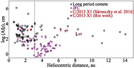
Variation of the Afρ parameter with heliocentric distance for long-period (black open squares) and short-period (purple open circles) comets (references from which the Afρ are taken are given in the text). Data for comet C/2013 X1 (PANSARRS) obtained in R filter are indicated by red symbols: filled squares represent data obtained in this work, and open diamonds show data from (Sárneczky et al. 2016). The vertical dashed line marks the snow line according to (Martin & Livio 2012).
4 POLARIMETRY OF THE COMET
4.1 Phase-angle dependence of polarization
Fig. 3b shows the map of polarization distribution across the coma of comet C/2013 X1 obtained in the R band on 2015 November 4, when the comet was at a distance of 2.66 au from the Sun. The minimum degree of polarization about −1.5 per cent is detected in the near-nucleus region of the coma, in the range up to about 10 000 km from the optocentre. Further, polarization gradually increases (in absolute value) with distance from the nucleus, reaching −6.5 per cent at about 50 000 km. The fan-shaped structure is visible in the image in the north-Sun direction, although it does not exactly coincide with the Sunward direction. The edges of this fan are curved towards the east and are nearly perpendicular to the direction of the Sun. This curvature can be explained by the trajectory of particles escaping from the rotating nucleus and being exposed to solar radiation. We determined the polarization degree of the comet averaged over an aperture with a radius of ∼9500 km and centred at the nucleus. It is −2.1 ± 0.05 per cent at a phase angle of α = 12.3°. The aperture polarimetry of the comet performed at the 2.6-m telescope provides the degree of polarization −2.20 ± 0.14 per cent at α = 10.1° and 2.89 ± 0.76 per cent at α = 29.1° on 2015 November 13 and 2016 January 13, respectively (see Fig. 5).
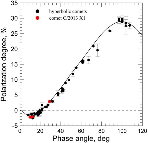
Phase-angle dependence of the degree of linear polarization for hyperbolic comets taken from DBCP V2.0 (Kiselev et al. 2017), Ivanova et al. (2017), and Zhuzhulina et al. (2022a, b) (black circles). The polarization degree of comet C/2013 X1 (PANSARRS) is marked by red symbols. The solid line displays the model phase-angle curve of polarization (see details in Section 4.2).
Fig. 5 demonstrates a phase-angle dependence of linear polarization based on data for hyperbolic comets taken from DBCP V2.0 (Kiselev et al. 2017) and some recent data obtained by Ivanova et al. (2017) and Zhuzhulina et al. (2022a, b), they are marked by black circles. We selected observations obtained with the broad-band filters centred at the central wavelength of the R filter used in our studies. To complete selected data at the largest phase angles, we also used observations in DBCP V2.0 obtained with the RC narrow-band filter. The points for comet C/2013 X1 are marked by red circles. As one can see, the results for the studied comet are in good agreement with the data obtained for other hyperbolic comets in the red bandpass.
4.2 Dust particle model
The shape matrix method, also known as the Sh-matrix method, was created using the T-matrix technique (Petrov et al. 2006). This method separates shape-related factors from size- and refractive index-related factors. This factorization describes the particle shape using a shape matrix, or Sh-matrix (e.g. Petrov, Shkuratov & Videen 2011, 2012). The Sh-matrix method has the same advantages as the T-matrix method, such as analytical averaging over particle orientation and accounting for size and refractive index dependences through analytical operations to create T-matrix elements.
The shape matrix can be determined by integration over the surface of the scattering particle and can be used to calculate the scattering properties of a particle with a given size and refractive index. It is often possible to find analytical expressions for calculating the shape matrix. The elements of Sh-matrix depend only on the morphology of the particle and, in many cases, can be solved analytically for particles of arbitrary shape (Petrov et al. 2011, 2012). The Sh-matrix method has been successfully used to study the scattering properties of dust particles and to isolate regolith composed of particles of irregular shapes. In this work, irregularly shaped samples were used to calculate their light-scattering properties.
Random Gaussian particles are a successful model of irregular particles described by Muinonen (1996, 1998). It is characterized by a mean radius and a logarithmic radius in spherical coordinates, and the logarithm of the particle radius is described by a series expansion in the associated Legendre polynomials with non-negative coefficients. Later, a model of conjugate random Gaussian particles was developed, which combines both large-scale and small-scale roughness (Petrov & Kiselev 2019). Examples of conjugate random Gaussian particles are shown in Fig. 6.

Examples of conjugate random Gaussian particles.
To interpret the observed phase-angle dependence of the linear polarization (Fig. 5), we applied the Sh-matrix method to light scattering by conjugated Gaussian random particles. In our dust coma simulation, we used a particle mixture consisting of amorphous carbon (refractive index m = 1.993 + 0.259i; Scott & Duley 1996), Mg-rich silicates (m = 1.674 + 0.002224i; Li & Greenberg 1997), and ice. These values of refractive indices are widely used for interpretation of cometary observations (e.g. Halder & Ganesh 2021). Particle sizes were taken from 0.49 μm (carbon), 0.83 μm (silicates), and 0.39 μm (ice) to 3 μm. We averaged the particles by orientations and sizes according to a power law with the exponent n = 3 for all particle types. Modelling revealed that the dust coma has to consist of 74 per cent amorphous carbon, 25 per cent of Mg-rich silicates, and 1 per cent of water ice to reproduce the observed values of linear polarization (solid line in Fig. 5). These results are in good agreement with the data of Woodward et al. (2021) derived from analyses of the IR spectral observations and thermal modelling. Indeed, Woodward et al. (2021) determined that the dust composition in comet C/2013 X1 was dominated by dark dust particles (modelled as amorphous carbon) with a carbon-to-silicon (C/Si) atomic ratio of 7.781 ± 6.091 which is much higher than that in carbonaceous chondrites. Thus, according to our modelled results of polarimetry and the findings by Woodward et al. (2021) and Wooden et al. (2021), we can conclude that the solid-state material that composes dust particles in comet C/2013 X1 is rich in carbon.
5 CONCLUSIONS
We provided the analysis of quasi-simultaneous spectral, photometric, and polarimetric observations of hyperbolic comet C/2013 X1 (PANSTARRS) performed at the 6-m telescope on 2015 November 4, and polarimetric observations at the 2.6-m telescope on 2015 November 13 and 2016 January 13. The main findings are the following:
In the spectrum of comet C/2013 X1, 54 emissions of CN, C2, C3, and NH2 molecules were identified within the wavelength range of 3800 – 7100 Å. The production rates of CN, C2, and C3 molecules are (5.01 ± 0.24) × 1026, (3.16 ± 0.07) × 1026, and (3.98 ± 0.25) × 1025 mol s−1, respectively. Using the blue, green, and red narrow-band cometary filters, the Afρ parameters (as a proxy for the dust production), corrected for the phase-angle effect, are estimated as 368 ± 11, 433 ± 12, and 1749 ± 25 cm, respectively. The normalized spectral gradient of the dust reflectivity was obtained at the level of 13 ± 3 per cent per 1000 Å for the |$BC{\!-\!}RC$| spectral range.
The images processed by digital filters show the presence of a fan-shaped structure of the triangular shape located at the position angle PA = 17°, which expands towards the Sun, and a short, weak tail directed in the opposite direction, PA = 225°.
The mean V − R colour over the coma of comet C/2013 X1 measured within the aperture with a radius of 13 820 km is (0.35 ± 0.04) mag, which corresponds, within the measurement errors, to a neutral colour of the cometary dust compared to the solar colour. There are variations in the dust colour over the coma: V − R changes along the fan from slightly red in the near-nucleus area to blue in the outer region.
On 2015 November 4, the degree of linear polarization varied over the coma: the minimum degree of polarization of about −1.5 per cent is detected in the near-nucleus region of the coma, approximately up to 10 000 km from the optocentre, and further, the polarization gradually increases (in absolute value) with cometocentric distance, reaching −6.5 per cent at about 50 000 km.
Using the Sh-matrix method with conjugated Gaussian random particles as light scatters, we found the chemical composition of dust particles in the coma which reproduces observed polarization and the phase-angle dependence of polarization for hyperbolic comets: it consists of 74 per cent amorphous carbon, 25 per cent of Mg-rich silicates, and 1 per cent of water ice.
Based on the production rate ratios of molecules C2 and C3 relative to CN, we conclude that comet C/2013 X1 most likely has a typical molecular composition. On the other hand, our results of polarimetric observations together with the data of Woodward et al. (2021) and Wooden et al. (2021) derived from analyses of the IR spectral observations indicate that dust particles in comet C/2013 X1 are rich in carbon. The thermal modelling of cometary dust using the ratio of the mass fractions of amorphous carbon and silicates revealed the very high elemental C/Si ratio in several comets, including C/2013 X1 (Woodward et al. 2021). Since atomic carbon is difficult to detect, these results suggest the large atomic carbon reservoir in the outer disc, the region where comets formed (Wooden et al. 2021, 2022), which is found in the carbonaceous component of the refractory material that composes the dust particle population of comet C/2013 X1, as well as of 67P/Churyumov–Gerasimenko (Bardyn et al. 2017) and dynamically new comets (Woodward et al. 2021).
ACKNOWLEDGEMENTS
The authors thank the anonymous referee for valuable comments on this work. OSh is grateful for the support funded by the EU NextGenerationEU through the Recovery and Resilience Plan for Slovakia under project no. 09I03-03-V01-00001. The work by OSh and OI was supported by the Slovak Grant Agency for Science VEGA (grant no. 2/0059/22) and by the Slovak Research and Development Agency under contract no. APVV-19-0072. The research by OI, IL, and VR was supported by Project 22BF023-02 of the Taras Shevchenko National University of Kyiv and the Ministry of Education and Science of Ukraine. The data from the 6-m telescope BTA were taken from the archive with free access, and the observations were carried out by Dr A. Moiseev. The authors note the great contribution of Prof. Viktor Afanasiev, who passed away on 2020 December 21, to the development and creation of the multimode focal reducer SCORPIO-2, as well as to this work.
DATA AVAILABILITY
The data underlying this article will be shared on reasonable request to the corresponding author.
Footnotes
SCORPIO: Spectral Camera with Optical Reducer for Photometrical and Interferometrical Observations.
