


ABSTRACT
Since its discovery in 1992, GRS 1915 + 105 has been among the brightest sources in the X-ray sky. However, in early 2018, it dimmed significantly and has stayed in this faint state ever since. We report on AstroSat and NuSTAR observation of GRS 1915 + 105 in its unusual low/hard state during 2019 May. We performed time-resolved spectroscopy of the X-ray flares observed in this state and found that the spectra can be fitted well using highly ionized absorption models. We further show that the spectra can also be fitted using a highly relativistic reflection dominated model, where for the lamp post geometry, the X-ray emitting source is always very close to the central black hole. For both interpretations, the flare can be attributed to a change in the intrinsic flux, rather than dramatic variation in the absorption or geometry. These reflection dominated spectra are very similar to the reflection dominated spectra reported for active galactic nuclei in their low flux states.
1 INTRODUCTION
Black hole (BH) X-ray binary (XRB) system consists of a BH and its companion which is a normal star, orbiting around their common centre of mass. The BH accretes matter from its companion via a geometrically thin, optically thick accretion disc (Novikov & Thorne 1973; Shakura & Sunyaev 1973). Depending on the mass of the companion, those having a less massive companion (M ≤ M⊙) usually accrete via Roche-lobe overflow and are referred as low mass X-ray binaries (LMXBs) while those having a more massive companion (M > 10 M⊙) usually accrete through stellar winds and are referred as high mass X-ray binaries (HMXBs; Petterson 1978; Blondin, Stevens & Kallman 1991; Liu, van Paradijs & van den Heuvel 2007; Tan 2021). The majority of BH-XRBs are observed as X-ray transients (Corral-Santana et al. 2016; Tetarenko et al. 2016) and most of them are LMXBs. LMXBs spend most of their lives in a quiescent state where there is a steady mass transfer from the companion onto the compact object. An increase in the temperature of the disc is believed to initiate thermal viscous instabilities that prompt a fast outflow of material from the companion onto the BH resulting in an X-ray outburst. (Shakura & Sunyaev 1976; Hameury, King & Lasota 1990). The outburst duration in a BH-XRB can range from several months to a few years. State changes are a common feature in BH-XRBs. During a typical outburst, they evolve in their spectral and timing properties, leading to the classification of various spectral states. (Remillard & McClintock 2006; Belloni & Motta 2016). Typically, an outburst begins with a low/hard state, progresses to a high/soft state, and ultimately reverts back to a low/hard state towards the end of the outburst. Intermediate states are often observed around the time of state transitions (Belloni et al. 2000).
Three main radiative components are often present in the X-ray spectrum of BH-XRBs. The black-body radiation from the accretion disc dominating the emission in the soft X-ray band (Shakura & Sunyaev 1973), power-law like component caused by inverse Compton scattering of the disc photons from the region near the central BH, typically referred to as corona, dominating the emission in the hard X-ray band (Shakura & Sunyaev 1976; Sunyaev & Titarchuk 1980; Lightman & Zdziarski 1987). The lower and upper cutoffs of this power-law component is determined by the temperature of the seed photons and electrons, respectively. The third component arises due to the fraction of the coronal photons irradiating the disc and being scattered into our line of sight. These photons are reprocessed in the disc’s atmosphere and produce reflection spectrum with characteristic features. The scattering produces a broad Compton hump peaking around ∼20–30 keV (Lightman & White 1988; Fabian et al. 1989) and many spectral lines, the strongest being a broad emission line at ∼6.4 keV due to iron (George & Fabian 1991; Ross & Fabian 2005). The line profile is set by special and general relativistic effects.
GRS 1915 + 105 is among one of the most well studied BH-XRBs, discovered in 1992 as an X-ray transient with the WATCH instrument onboard International Astrophysical Observatory ‘GRANAT’ (Castro-Tirado, Brandt & Lund 1992). GRS 1915 + 105 hosts a BH of mass |$12.5^{+2.0}_{-1.8}$| M⊙, located at radio parallax distance of |$8.6^{+2.0}_{-1.6}$| kpc with disc inclination of 60° (Reid et al. 2014). GRS 1915 + 105 has the longest orbital period of 33.9 d (Steeghs et al. 2013) among all the LMXBs and therefore has the largest accretion disc and high accretion rate. It is a unique source among all BH-XRBs because of its interesting properties, viz. high luminosity, distinctive X-ray variability classes (Belloni et al. 2000), high frequency quasi-periodic oscillations (Remillard & McClintock 2006), probably due to large accretion disc and high accretion rate. After a long period of about 26 yr in outburst, in 2018 July (∼MJD 58300) GRS 1915 + 105 entered into unusually low X-ray flux state. Negoro et al. (2018) reported the lowest soft X-ray flux of the source in 22 yr of continuous monitoring with MAXI/GSC and RXTE/ASM. The strong similarities between this flux drop and outburst evolution of other BH-XRBs led Negoro et al. (2018) to conclude that GRS 1915 + 105 was finally entering into a quiescent state, but in 2019 May (∼MJD 58600) the source again showed strong activity with a further drop in average X-ray flux and has remained in this faint state since then. Strong radio flares in this state also indicate that the mass accretion rate can still be high (Motta et al. 2019). In this obscured state GRS 1915 + 105 has flux an order of magnitude less than observed previously also strong erratic X-ray flares have been observed in this state (Iwakiri et al. 2019; Jithesh et al. 2019; Neilsen et al. 2019). This kind of variability has not been seen in this source before. X-ray observations in this state showed Compton thick obscuration, hard spectra, with strong emission and absorption lines characterized by a clear increase in intrinsic absorption with column densities over an order of magnitude larger than those usually observed in the source before. (Miller et al. 2019a, b, 2020; Koljonen & Tomsick 2020; Balakrishnan et al. 2021; Motta et al. 2021).
Reflected spectra characterized by high reflection fraction (exceeding unity) have been observed in many individual observations of low flux states in active galactic nuclei (AGN; Seyferts) MCG-6-30-15 (Fabian & Vaughan 2003), 1H 0707–495 (Fabian et al. 2004), and 1H0419-577 (Fabian et al. 2005). This high reflection fraction was explained on the basis of light bending model as discussed by Miniutti & Fabian (2004). In their model X-ray source is assumed to be very close to the maximally rotating central BH, so a large number of photons will be captured by the central BH and most of the remaining photons will be focused towards the innermost regions of the accretion disc. The strong light bending effects in the innermost parts of the accretion disc enhance the reflection fraction thus producing the reflection dominated spectra. Miniutti & Fabian (2004) in their light bending model identified three different flux states i.e. low, intermediate, and high in which the reflection dominated component of the spectrum is correlated, anticorrelated or almost independent with respect to the direct continuum.
Highly reflection dominated spectra have been observed in some BH-XRBs also. Rossi et al. (2005); Reis et al. (2013) analysed the Rossi X-ray Timing Explorer (RXTE) data of XTE J1650-500 and showed that the reflection fraction increases sharply at transition between soft intermediate and hard intermediate states. They also showed that at low power-law flux levels the Fe K α line flux and power-law flux are positively correlated and line equivalent width and power-law flux are anticorrelated which is in agreement with the light bending model proposed by Miniutti & Fabian (2004).
Koljonen & Tomsick (2020) analysed Nuclear Spectroscopic Telescope Array (NuSTAR) spectra for a number of BH X-ray binaries (V4641 Sgr, Cyg X-3, V404 Cyg, and GRS 1915+105) using a complex combination of spectral components such as smeared edges, partial covering, distant and relativistic reflection, and obscuration/emission from surrounding tori. In general, their preference is that these sources exhibit either highly absorbed partial covering or can be explained in terms of a torus covering the source. In particular, for GRS 1915 + 105, they analysed three epochs and found that the latter two epochs require highly absorbed partial covering with column density |$\sim 5 \times 10^{23}\, \mathrm{cm}^{-2}$| or a torus with radial velocity. The first epoch could be represented by their torus model, but also by relativistic reflection.
The AstroSat observation used in this study was taken just a day after MAXI/GSC detected the re-brightening of GRS 1915 + 105 (Iwakiri et al. 2019). The bottom panel of the MAXI lightcurve shown in Fig. 1 indicates that the source count rate was almost three times large during the AstroSat observation period (depicted by solid lines) compared to the NuSTAR observation period (depicted by dashed lines). The strong erratic flares were observed in both the Large Area X-ray Proportional Counter (LAXPC) and Soft X-ray Telescope (SXT) lightcurves, where the source intensity increased by a factor of ∼5. The flaring activity became weak after first 60 ks time of the lightcurve and then disappeared completely. The detailed spectral study of this observation was not done before. In this work we report the results of our analysis of one of the flares for which simultaneous LAXPC and SXT data is available. The detailed analysis of the other flares will be discussed in follow-up work. One of the NuSTAR observations [Koljonen & Tomsick (2020) Epoch 1 data] has spectrum similar to the one observed by AstroSat and hence we re-analyse the data using the models used for AstroSat. The structure of this paper is as follows. In Section 2 the observations and data reduction procedures are described. The findings from spectral analysis of our time-resolved spectra are discussed in Section 3. These results are then discussed and interpreted in Section 4. We then discuss our conclusions in Section 5.
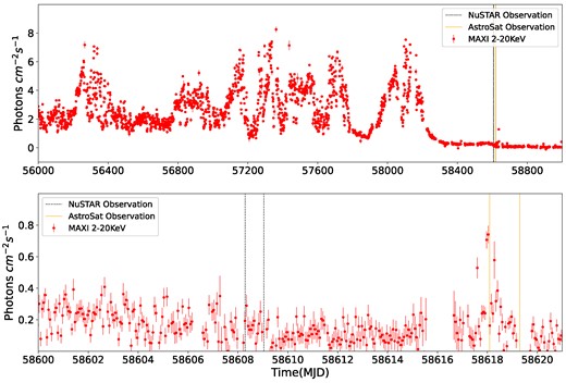
Upper panel: 1-d average MAXI/GSC long term lightcurve of GRS 1915 + 105 from MJD 56 000 to 59 500 (2012–2022). The dashed and solid solid lines corresponds to the time of our NuSTAR and AstroSat observations shown in Table 1. Lower panel: One orbit binned MAXI/GSC lightcurve from MJD 58 600 to 58 620 showing the time of our NuSTAR and AstroSat observation marked between dashed and solid vertical lines, respectively.
2 OBSERVATION AND DATA REDUCTION
In this work, we used AstroSat and NuSTAR observations of GRS 1915 + 105 conducted during 2019 May. The observation details are given in Table 1. These observations are also overplotted on the 1-day averaged 2–20 keV MAXI lightcurve shown in Fig. 1(Top panel). The one orbit binned MAXI lightcurve showing the observation time of both the NuSTAR and AstroSat observations is also shown in Fig. 1(Bottom panel).
Observation log.
| Instrument | Obs ID | Start time | End time | MJD | Exposure |
|---|---|---|---|---|---|
| Date | Date | (ks) | |||
| AstroSat | T03_116T01_9000002916 | 02:04:22 | 07:14:37 | 58618.09064 | 22.6 |
| 15-05-2019 | 16-05-2019 | ||||
| NuSTAR | 90 501 321 002 | 07:06:09 | 01:01:09 | 58608.29974 | 28.7 |
| 05-05-2019 | 06-05-2019 |
2.1 NuSTAR
The NuSTAR consists of two co-aligned, identical X-ray telescopes focusing the hard X-rays in a wide energy range of 3–79 keV. Each of the telescopes has its own focal plane modules FPMA and FPMB (Harrison et al. 2013). We selected the NuSTAR observation of GRS 1915 + 105 during 2019 May 5–6 (Observation ID: 90501321002) in its unusual low state. We reduced the raw data following the NuSTAR Data Analysis Software Guide1 using the NuSTAR data analysis software (nustardas v2.1.1) provided under heasoft v6.29 with CALDB version (20221229). The filtered clean event files were produced using the nupipeline routine by setting the parameters ‘TENTACLE=YES’ and ‘SAAMODE = OPTIMISED’ to remove times with high background and the science products for both FPMA and FPMB were then extracted using the nuproducts routine. The source spectrum was extracted by taking a circular region of radius 100 arcsec centred on the source and the background spectrum from the circular region of radius 100 arcsec of the detector not contaminated by source counts. The data from both the detectors FPMA and FPMB is grouped with background, ancillary response file (ARF) and response matrix file (RMF) using grppha command. An optimal binning scheme using ftgrouppha was then used to group the energy bins together. The lightcurve of the NuSTAR observation is shown in Fig. 2.
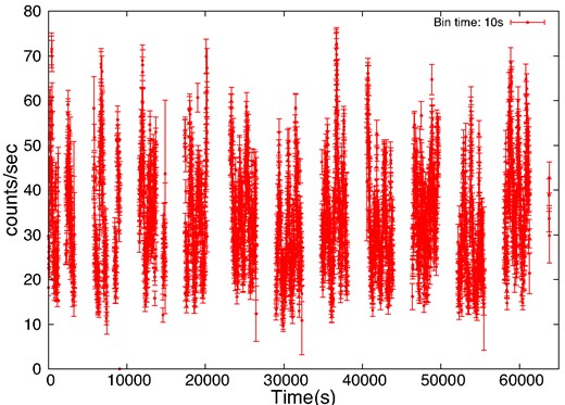
NuSTAR lightcurve of the observation used for this study. The time along X-axis is the time since 58608.29974 MJD (Start time of observation).
2.2 AstroSat
AstroSat is India’s first multiwavelength astronomical satellite dedicated to observing cosmic sources in wide energy ranges of the electromagnetic spectrum, from optical to X-ray bands (Agrawal 2006). AstroSat has five different payloads with SXT (Singh et al. 2016, 2017) and LAXPC (Yadav et al. 2016; Antia et al. 2017) providing an opportunity to study the X-rays in energy range of 0.3–8.0 keV and 3.0–80.0 keV, respectively.
The SXT level 2 data for 16 orbits in photon counting mode was downloaded from AstroSat data archive-ISSDC. The data reduction was achieved with tools provided by SXT POC team at TIFR2. The individual clean event files for each orbit were then combined using Sxtpyjuliamerger_v01 to generate a single merged clean event file. To extract the science products, further analysis of data was performed using xselect v2.4m. We extracted a circular source region of radius 18 arcmin centred on the source. For segments S5, S6, and S9, since the net count rate was >40 counts s−1, to account for pileup effect we extracted annulus source region of inner radius 2.5 arcmin and outer radius of 18 arcmin. We have used RMF3 and blank sky background spectrum file4 provided by the SXT instrument team for our analysis. The vignetting corrected ancillary response file (ARF) was created with sxt ARFM odule using the ARF file provided by SXT team. The background spectrum, vignetting corrected ARF and RMF were then grouped together using interactive command grppha such that each bin contains a minimum of 25 counts.
LAXPC consists of three proportional counters LAXPC10, LAXPC20, and LAXPC30. We have used only LAXPC20 data for our analysis as LAXPC10 and LAXPC30 were not functional at the time of our observation. We downloaded the level 1 data for all the 16 orbits from the AstroSat data archive and used the LAXPC software (2022 August 15 version)5 to convert it to level 2. laxpc_make_lightcurve and laxpc_make_spectra codes were then used to extract the lightcurve and spectrum fot each segment.
The simultaneous LAXPC and SXT lightcurves of the observation along with MAXI lightcurve of the source for the time of AstroSat observation is shown in Fig. 3. The LAXPC and SXT lightcurves are 2.3775 s binned, the minimum time resolution of SXT instrument. Among the erratic X-ray flares in LAXPC and SXT lightcurves, we have selected the flare marked between dotted lines in Fig. 3 for our study. We chose this specific flare because it occurred simultaneously in both the LAXPC and SXT instruments, and had both the highest count rate and longer flaring duration among all other flares having simultaneous data available for both the instruments. We then divided the flare into 12 different segments, as shown in Fig. 4 and both LAXPC and SXT products were extracted for each segment using single gti for both instruments.
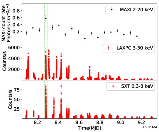
MAXI and Astrosat lightcurves: Top panel shows zoomed 1.5 h binned lightcurve in energy range 2.0–20.0 keV for the time of AstroSat observation, the middle panel corresponds to background subtracted LAXPC lightcurve in 3.0–30.0 keV energy band and bottom panel corresponds to SXT lightcurve in 0.3–8.0 keV energy band. The flare marked between dotted vertical lines was only used for this analysis.
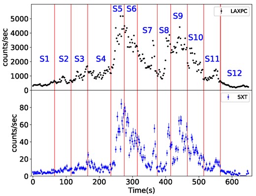
Zoomed in view of the flare marked in Fig. 3 considered for this study. The time along X-axis is the time since 295 598 385 AstroSat seconds (start of flare). The flare is divided into twelve different segments from S1 to S12 and are marked by the vertical lines. Upper panel is for LAXPC while the lower panel shows the SXT lightcurve.
3 SPECTRAL ANALYSIS
All the spectral fits were performed in xspec version: 12.12.0 (Arnaud 1996). A constant factor was introduced in all the joint spectral fits to account for the cross-calibration uncertainty between different instruments. For AstroSat analysis the constant was fixed at unity for SXT and was allowed to vary for LAXPC, while for NuSTAR constant was fixed at unity for FPMA and was allowed to vary for FPMB. In addition to this a gain fit was also performed on both the LAXPC and SXT to modify the gain of the response file (Antia et al. 2021). A systematic error of 3 per cent was used in the joint fitting of AstroSat SXT and LAXPC spectra to take care of the uncertainties in the response matrix. The error on all the parameters are reported at 90 per cent confidence level unless specified otherwise.
The NuSTAR data used in this study was analysed by Koljonen & Tomsick (2020) and they reported the presence of strong iron line feature, a strong iron absorption line and curvature in the hard X-rays around ∼20–30 keV. This curvature being the typical feature for hard state XRB might be caused by heavy absorption of the incident spectrum or by Compton down-scattering in the accretion disc or in the surrounding medium. For the NuSTAR observation, Koljonen & Tomsick (2020) used relxillCp, a Gaussian line to model the strong iron absorption line around around 6.5 keV, the interstellar absorption was taken care of using phabs. A smeared iron absorption edge component smedge was also used to model the absorption features in the spectra around 7–8 keV.
3.1 Spectral fits with absorption dominated model
The spectra for all the segments from Astrosat and NuSTAR were modelled using a Comptonization component thcomp, a multicoloured black-body component diskbb and a reflection component xillverCp, to model the distant reflection from the disc. The Galactic absorption was taken care of by the absorption model tbabs and the local obscured absorption features observed in the spectrum was modelled using a photo-ionized absorption model zxipcf (Reeves et al. 2008). In addition to this, a Gaussian line was used to model the strong iron absorption line at ∼6.5 keV for the NuSTAR data. So the total model used is constant × tbabs × zxipcf (thcomp × diskbb + xillverCp) in xspec notation for the AstroSat data and an additional Gaussian component for the NuSTAR data. The neutral hydrogen column density was fixed at 5.0 × 1022 cm−2. This is in comparison to the earlier observed values (Zoghbi et al. 2017; Koljonen & Tomsick 2020). Initially zxipcf covering fraction was left free to vary for AstroSat data, we could not bound its upper limit and its value was always consistent with unity, so we fixed it at 1, i.e. we assumed the total covering of the X-ray source, while for the NuSTAR data it was left free to vary. The inner disc temperature of the disc i.e the parameter Tin in model diskbb was not constrained by the data, and hence was fixed at 1 keV. xillverCp was included only as a reflection component by fixing the reflection fraction at −1. The iron abundance AFE, in units of solar abundance was fixed at 1. The density of the disc in logarithmic units (logN) and the inclination of the disc were fixed at 17 cm−3 and 60°. All the parameters of the Comptonization component describing the coronal properties were tied to the corresponding xillverCp values. The electron temperature (kTe) for the AstroSat data was fixed at 400 keV, since its value was high for NuSTAR data and the upper limit was pegged at 400 keV. Adding a systematic error of 1 per cent in the NuSTAR data improved the fit by Δχ2 ∼138 so we have added 1 per cent systematic error to the spectral fitting of NuSTAR data. The systematic also includes complex spectral model systematic rising due to the model assumptions regarding geometry and homogeneity, which may not accurately describe the physical source. For NuSTAR data, we have included 1 per cent systematic to take into account such spectral model uncertainties. We calculated the unabsorbed flux in energy range 0.7–30 keV and 3–79 keV for AstroSat and NuSTAR data, respectively, and the corresponding luminosities were then calculated. The best-fitting spectral parameters for the AstroSat and NuSTAR observation are presented in Tables 2 and 3. The fitted spectra for one segment of AstroSat data and the NuSTAR observation are shown in Fig. 5. The column density for the ionized absorption ranged from 1023 to |$10^{24}\, \mathrm{cm}^{-2}$|.
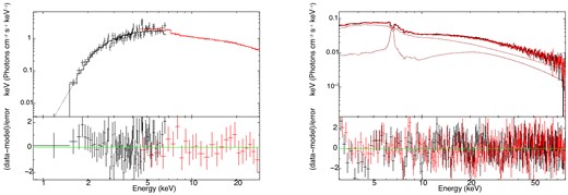
The left panel represents the AstroSat spectrum of segment 6 from the simultaneous fit of 0.7–7 keV SXT and 4–30 keV LAXPC data modelled with constant × tbabs × zxipcf (thcomp × diskbb + xillvercp) and the right panel shows the NuSTAR FPMA and FPMB spectrum in energy range 3–79 keV modelled using constant × tbabs × zxipcf (thcomp × diskbb + xillvercp + gaussian).
Best-fitting spectral parameters for the model combination constant × tbabs × zxipcf (thcomp × diskbb + xillvercp) for AstroSat data 0.7–30.0 keV.
| Segment | zxipcf | zxipcf | diskbb | xillverCp | xillverCp | xillverCp | χ2/degrees | Flux | Luminosity |
|---|---|---|---|---|---|---|---|---|---|
| NH | log ξ | norm | Γ | log ξ | norm | of freedom | × 10−9 | × 1037 | |
| × 10−3 | |||||||||
| 1 | |$87.74^{ -57.70}_{+ 14.09}$| | |$3.07^{ -0.08}_{+ 0.1}$| | <31.10 | |$1.88^{ -0.07}_{+ 0.06}$| | >3.56 | |$22.40^{ -4.61}_{+ 4.97}$| | 36.39/31 | |$9.59^{ -0.15}_{+ 0.15}$| | |$8.49^{ -0.13}_{+ 0.13}$| |
| 2 | |$52.11^{ -17.51}_{+ 14.42}$| | |$2.99^{ -0.15}_{+ 0.13}$| | <49.61 | |$1.90^{ -0.04}_{+ 0.04}$| | >4.35 | |$37.11^{ -7.29}_{+ 6.95}$| | 42.46/36 | |$15.38^{ -0.22}_{+ 0.23}$| | |$13.62^{ -0.20}_{+ 0.20}$| |
| 3 | |$35.51^{ -8.44}_{+ 11.14}$| | |$2.86^{ -0.11}_{+ 0.14}$| | <70.33 | |$1.94^{ -0.03}_{+ 0.03}$| | |$3.96^{ -0.10}_{+ 0.30}$| | |$58.11^{ -9.77}_{+ 8.32}$| | 35.20/42 | |$21.78^{ -0.29}_{+ 0.29}$| | |$19.28^{ -0.25}_{+ 0.26}$| |
| 4 | |$29.90^{ -5.74}_{+ 4.55}$| | |$2.40^{ -0.15}_{+ 0.13}$| | <136.85 | |$1.90^{ -0.05}_{+ 0.05}$| | |$3.99^{ -0.15}_{+ 0.19}$| | |$82.55^{ -13.45}_{+ 19.60}$| | 65.95/51 | |$31.61^{ -0.47}_{+ 0.59}$| | |$27.99^{ -0.42}_{+ 0.52}$| |
| 5 | |$12.08^{ -3.39}_{+ 3.39}$| | |$2.54^{ -0.2}_{+ 0.18}$| | <242.52 | |$1.89^{ -0.02}_{+ 0.03}$| | |$4.12^{ -0.16}_{+ 0.24}$| | |$144.27^{ -27.82}_{+ 20.52}$| | 80.92/82 | |$55.96^{ -0.61}_{+ 0.63}$| | |$49.55^{ -0.54}_{+ 0.55}$| |
| 6 | |$12.72^{ -2.85}_{+ 3.22}$| | |$2.31^{ -0.13}_{+ 0.13}$| | <199.51 | |$1.93^{ -0.03}_{+ 0.03}$| | |$4.12^{ -0.16}_{+ 0.17}$| | |$188.59^{ -26.56}_{+ 23.59}$| | 84.75/90 | |$72.66^{ -0.77}_{+ 0.79}$| | |$64.33^{ -0.68}_{+ 0.70}$| |
| 7 | |$16.14^{ -3.78}_{+ 3.74}$| | |$2.40^{ -0.14}_{+ 0.15}$| | <173.92 | |$1.87^{ -0.03}_{+ 0.03}$| | |$3.82^{ -0.10}_{+ 0.10}$| | |$133.01^{ -21.93}_{+ 16.77}$| | 89.32/80 | |$47.26^{ -0.51}_{+ 0.52}$| | |$41.85^{ -0.46}_{+ 0.46}$| |
| 8 | |$26.07^{ -6.24}_{+ 3.95}$| | |$2.43^{ -0.10}_{+ 0.12}$| | <452.25 | |$1.92^{ -0.04}_{+ 0.04}$| | |$3.95^{ -0.12}_{+ 0.19}$| | |$148.10^{ -45.27}_{+ 24.65}$| | 47.57/59 | |$55.48^{ -0.66}_{+ 0.66}$| | |$49.12^{ -0.58}_{+ 0.59}$| |
| 9 | |$13.35^{ -2.81}_{+ 2.99}$| | |$2.24^{ -0.11}_{+ 0.12}$| | <155.20 | |$1.89^{ -0.03}_{+ 0.03}$| | |$4.08^{ -0.13}_{+ 0.18}$| | |$162.29^{ -22.17}_{+ 20.41}$| | 100.14/89 | |$62.28^{ -0.65}_{+ 0.67}$| | |$55.14^{ -0.58}_{+ 0.60}$| |
| 10 | |$13.28^{ -3.20}_{+ 3.51}$| | |$2.36^{ -0.13}_{+ 0.14}$| | <142.98 | |$1.97^{ -0.02}_{+ 0.02}$| | |$3.82^{ -0.08}_{+ 0.08}$| | |$142.10^{ -17.88}_{+ 20.54}$| | 83.37/82 | |$51.87^{ -0.59}_{+ 0.59}$| | |$45.92^{ -0.51}_{+ 0.53}$| |
| 11 | |$29.92^{ -13.45}_{+ 9.74}$| | |$2.87^{ -0.12}_{+ 0.11}$| | <94.18 | |$1.89^{ -0.03}_{+ 0.04}$| | |$3.65^{ -0.11}_{+ 0.14}$| | |$70.59^{ -11.42}_{+ 10.79}$| | 38.57/47 | |$23.86^{ -0.31}_{+ 0.32}$| | |$21.13^{ -0.28}_{+ 0.28}$| |
| 12 | |$17.59^{ -10.06}_{+ 11.10}$| | |$2.34^{ -0.35}_{+ 0.25}$| | |$76.73^{ -35.57}_{+ 46.92}$| | |$1.95^{ -0.13}_{+ 0.10}$| | |$2.95^{ -0.15}_{+ 0.41}$| | |$31.01^{ -8.45}_{+ 12.72}$| | 27.67/29 | |$9.62^{ -0.16}_{+ 0.17}$| | |$8.52^{ -0.14}_{+ 0.15}$| |
All the column densities are measured in 1022 atoms cm−2. The Flux reported here is the unabsorbed flux in the energy range 3–79 keV. All the fluxes are measured in |$\mathrm{erg\, {cm}^{-2}\, s}^{-1}$| and all the luminosities in |$\mathrm{erg\, s}^{-1}$|. The ionization parameter is measured in erg cm s−1.
Best-fitting spectral parameters for the model combination constant × tbabs × zxipcf (thcomp × diskbb + xillvercp + gaussian) for NuSTAR data 3–79 keV.
| zxipcf | ||
|---|---|---|
| NH | 1022 cm−2 | |$64.42^{ -8.62}_{+ 4.38}$| |
| log ξ | |$3.09^{ -0.06}_{+ 0.03}$| | |
| fcov | |$0.73^{ -0.05}_{+ 0.06}$| | |
| diskbb | ||
| norm | |$68.67^{ -1.97}_{+ 3.8}$| | |
| xillvercp | ||
| Γ | |$2.05^{ -0.01}_{+ 0.01}$| | |
| kTe | >345.86 | |
| log ξ | |$2.78^{ -0.03}_{+ 0.02}$| | |
| norm | × 10−3 | |$5.64^{ -0.58}_{+ 0.59}$| |
| gauss | ||
| E | keV | |$6.57^{ -0.02}_{+ 0.02}$| |
| σ | <0.09 | |
| norm | × 10−4 | |$-17.21^{ -3.33}_{+ 3.56}$| |
| Flux | × 10−9 | |$2.91^{ -0.01}_{+ 0.01}$| |
| Luminosity | × 1037 | |$2.59^{- 0.01}_{+ 0.01}$| |
| χ2/degrees of freedom | 521.23/464 |
The Flux reported here is the unabsorbed flux in the energy range 3–79 keV, measured in erg cm−2 s−1 and the luminosity in erg s−1. The ionization parameter is measured in erg cm s−1.
3.2 Spectral fits with reflection dominated model
To highlight the reflection features in our spectra we modelled both the AstroSat and NuSTAR data using the galactic absorption model Tbabs, a cutoff power-law (cutoffpl) and a constant. We fitted the LAXPC and SXT spectra in 0.7–30 keV for all the segments and NuSTAR spectrum in 3–79 keV. The ratio plots for one of the segments of AstroSat data and the NuSTAR data are shown in Fig. 6. For both spectra, excess flux is seen around∼6.5 and ∼20 keV, indicating the presence of broadened reflection components.
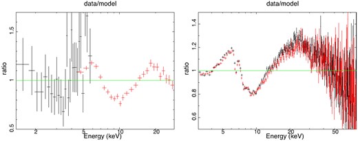
The Ratio plots of AstroSat spectrum for segment 11 (left) and NuSTAR spectrum (right) using model constant × tbabs × cutoffpl.
Like the typical hard state spectra of BH-XRBs, we first tried to fit the spectrum with a Comptonization component thcomp (Zdziarski et al. 2020), a multicoloured black-body component diskbb (Mitsuda et al. 1984) modified by the galactic absorption model Tbabs (Wilms, Allen & McCray 2000). There were strong residues in 6.4 keV energy range in the spectra of all the segments, due to the presence of Fe k α emission line, and was taken care of using Gaussian. A constant was also added to the spectra, so our total model in xspec notation is constant × tbabs (thcomp × diskbb + gaussian). We fitted all the segments of our AstroSat data with this model and it provided good statistical fit to all the spectra with |$\chi ^{2}_{ \mathrm{ reduced}}$| comparable to 1 for all segments. However, the electron temperature of the Comptonizing component turned out to be ∼5 keV with high optical depth τ > 12, making the component peak at ∼20 keV. Thus, the Comptonized component seemed to be modelling the broad reflection component and hence may not be physical.
We fitted the joint spectra extracted from NuSTAR FPMA and FPMB in energy range 3–79 keV and for joint spectra of SXT and LAXPC the energy range considered was 0.7–7 and 4–30 keV. We have used the model Tbabs to incorporate the Galactic absorption combined with relativistic reflection model relxill v 2.2.0 (Dauser et al. 2014; García et al. 2014) to fit both AstroSat and NuSTAR data. We used the relxillCp flavour of the relxill model, which internally includes the original continuum emission modelled using nthcomp and also the reflected emission from the disc modified for the relativistic effects in the inner accretion disc near the central BH. Thus the total model used in xspec notation is constant × tbabs × relxillcp. While fitting the NuSTAR observation with this model we found strong residuals in the energy range 6–8 keV. We found a strong iron absorption line at around 6.5 keV, so we modelled that using Gaussian and a smeared iron absorption edge smedge with index for photo-electric cross-section fixed at −2.67. So the total model we have used for the NuSTAR data is constant × smedge × tbabs (relxillCp + gaussian) in the xspec notation. The constant factor used for the cross-calibration between different instruments was well comparable to 1 for both NuSTAR and AstroSat observations. Initially, we tried to constraint the reflection fraction, but its value found from the fit was always very high and we thus could not constraint the upper bound on the parameter. We then fitted only the reflection component in relxillCp by fixing the model parameter ‘refl|$\_$|frac’ to negative value of −1. The spin is fixed to 0.998 (see also McClintock et al. 2006) to avoid model degeneracies, and this does not provide any indication of the actual value of the intrinsic angular momentum of the BH. The disc inclination of the system is fixed at 60° (Reid et al. 2014). The inner radius of the accretion disc Rin was kept free to vary and was always found close to the innermost stable circular orbit (ISCO) and the outer radius Rout was fixed at 400Rg, where Rg = GM/c2 is the gravitational radius of the BH. The emissivity profile in the relxillCp model is given by ϵ(r) ∝ |$r^{-q_{in}}$| for r < Rbr and ϵ(r) ∝ |$r^{-q_{out}}$| for r > Rbr where Rbr is the break radius and qin and qout, the index for inner and outer regions of the disc. We assumed the single power-law emissivity profile with qin = qout and free to vary. Initially, the density of the accretion disc (logN) was free to vary, and we found the average of the best-fitting value from all the segments of AstroSat observation ∼17 cm−3. So we fixed logN to 17 cm−3. The iron abundance AFE of the source was fixed to solar abundances. For reflection spectra, the relxill model allows the ionization parameter (ξ = 0) neutral to (ξ = 4.7) heavily ionized in logarithmic units, where ξ = 4πF/n, F is the irradiating flux and n is the density of the disc. The electron temperature of the corona (kTe) was very high and its upper limit could not be constrained with our NuSTAR data, and the value found was always large than 300 (keV), so we fixed it to 400 (keV) for all the segments. Adding a systematic error of 1 per cent in the NuSTAR data improved the fit by Δχ2 ∼141, so we have added 1 per cent systematic error to the spectral fitting of NuSTAR data. We calculated the flux using xspec model cflux and the Luminosity was then calculated assuming the distance of the source |$8.6^{+2.0}_{-1.6}$| kpc. The best-fitting spectral parameters for the AstroSat and NuSTAR observation are presented in Tables 4 and 5. The fitted spectra for one segment of AstroSat data and the NuSTAR observation are shown in Fig. 7. The parameters from the spectral fit of both absorption dominated and reflection dominated models are plotted as a function of time in Figs 8 and 9.
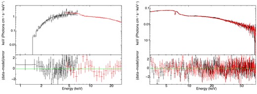
The left panel represents the AstroSat spectrum of segment 6 from the simultaneous fit of 0.7–7 keV SXT and 4–30 keV LAXPC data modelled with constant × tbabs × relxillcp and the right panel shows the NuSTAR FPMA and FPMB spectrum in energy range 3–79 keV modelled using constant × smedge × tbabs (relxillcp + gaussian).
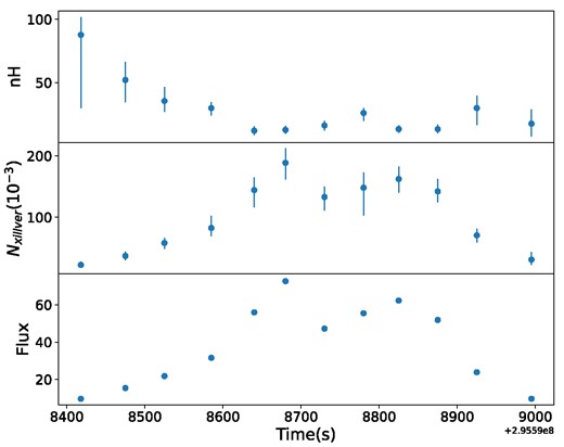
Variation of various spectral parameters as a function of time for the model combination constant × tbabs × zxipcf (thcomp × diskbb + xillverCp) using 0.3–30.0 keV AstroSat data. From top to bottom: Panels 1, 2, and 3 corresponds to nH of the ionized absorber (1022 cm−2), xillverCp norm and 0.7–30 keV unabsorbed flux (|$10^{-9} \, \mathrm{erg\, {cm}^{-2}\, s}^{-1}$|). The flux errors are small and thus not visible in plot. Note that although there is variation of the absorption column density, the large variation of the unabsorbed flux indicates an intrinsic origin for the flare.
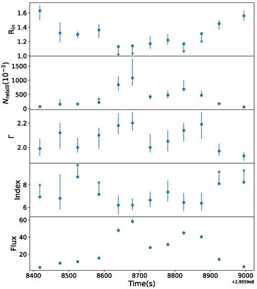
Variation of various spectral parameters as a function of time for the model combination constant × tbabs × relxillCp using 0.3–30.0 keV AstroSat data. From top to bottom: Panel 1, 2, 3, 4, and 5 corresponds to ISCO, relxillCp norm, Photon index, emisivity index of disc and 0.7–30 keV unabsorbed flux (|$10^{-9} \, \mathrm{erg\, {cm}^{-2}\, s}^{-1}$|). The flux errors are small and thus not visible in plot.
Best-fitting spectral parameters for the model combination constant × tbabs × relxillCp for AstroSat data 0.3–30.0 keV.
| Segment | Tbabs | relxillCp | relxillCp | relxillCp | relxillCp | relxillCp | χ2/degrees | Flux | Luminosity |
|---|---|---|---|---|---|---|---|---|---|
| NH | Rin | Emissivity | Γ | log ξ | norm | of freedom | × 10−9 | × 1037 | |
| (ISCO) | Index | × 10−3 | |||||||
| 1 | |$6.19^{ -0.93}_{+ 0.87}$| | |$1.63^{ -0.13}_{+ 0.08}$| | >6.92 | |$1.99^{ -0.06}_{+ 0.08}$| | |$2.80^{ -0.07}_{+ 0.11}$| | |$49.28^{ -7.41}_{+ 10.07}$| | 32.74/31 | |$4.74^{ -0.52}_{+ 0.53}$| | |$4.20^{ -0.46}_{+ 0.47}$| |
| 2 | |$6.95^{ -0.91}_{+ 1.17}$| | |$1.32^{ -0.13}_{+ 0.15}$| | |$6.80^{ -0.98}_{+ 2.14}$| | |$2.12^{ -0.13}_{+ 0.08}$| | |$2.78^{ -0.12}_{+ 0.16}$| | |$102.18^{ -29.27}_{+ 28.70}$| | 42.30/36 | |$9.74^{ -0.92}_{+ 0.92}$| | |$8.62^{ -0.81}_{+ 0.82}$| |
| 3 | |$6.60^{ -0.61}_{+ 0.64}$| | |$1.30^{ -0.05}_{+ 0.04}$| | >8.70 | |$2.00^{ -0.04}_{+ 0.08}$| | |$3.00^{ -0.08}_{+ 0.06}$| | |$104.68^{ -14.74}_{+ 21.35}$| | 33.42/42 | |$11.44^{ -0.89}_{+ 0.90}$| | |$10.13^{ -0.79}_{+ 0.79}$| |
| 4 | |$7.49^{ -0.69}_{+ 0.79}$| | |$1.36^{ -0.11}_{+ 0.08}$| | >7.15 | |$2.10^{ -0.11}_{+ 0.06}$| | |$2.75^{ -0.12}_{+ 0.12}$| | |$181.65^{ -43.52}_{+ 45.12}$| | 70.17/53 | |$15.55^{ -1.02}_{+ 1.02}$| | |$13.76^{ -0.89}_{+ 0.91}$| |
| 5 | |$6.73^{ -0.42}_{+ 0.48}$| | <1.13 | |$6.19^{ -0.81}_{+ 0.89}$| | |$2.18^{ -0.07}_{+ 0.10}$| | |$2.79^{ -0.09}_{+ 0.13}$| | |$538.81^{ -95.06}_{+ 173.19}$| | 93.87/82 | |$47.81^{ -2.23}_{+ 2.22}$| | |$42.33^{ -1.97}_{+ 1.97}$| |
| 6 | |$7.22^{ -0.36}_{+ 0.35}$| | <1.14 | |$6.19^{ -0.43}_{+ 0.59}$| | |$2.20^{ -0.06}_{+ 0.09}$| | |$2.78^{ -0.07}_{+ 0.07}$| | |$664.90^{ -103.02}_{+ 196.72}$| | 97.37/90 | |$58.22^{ -2.55}_{+ 2.55}$| | |$51.55^{ -2.26}_{+ 2.26}$| |
| 7 | |$6.96^{ -0.45}_{+ 0.51}$| | |$1.17^{ -0.07}_{+ 0.10}$| | |$6.64^{ -0.60}_{+ 0.74}$| | |$2.00^{ -0.04}_{+ 0.11}$| | |$2.94^{ -0.12}_{+ 0.12}$| | |$262.17^{ -30.63}_{+ 71.91}$| | 101.68/80 | |$27.80^{ -1.33}_{+ 1.33}$| | |$24.61^{ -1.17}_{+ 1.18}$| |
| 8 | |$8.26^{ -0.80}_{+ 0.84}$| | |$1.22^{ -0.06}_{+ 0.08}$| | |$7.36^{ -0.82}_{+ 1.01}$| | |$2.05^{ -0.08}_{+ 0.09}$| | |$2.91^{ -0.13}_{+ 0.14}$| | |$308.41^{ -57.81}_{+ 91.09}$| | 56.15/59 | |$31.38^{ -1.87}_{+ 1.88}$| | |$27.78^{ -1.65}_{+ 1.67}$| |
| 9 | |$7.54^{ -0.50}_{+ 0.56}$| | <1.17 | |$6.43^{ -0.77}_{+ 0.84}$| | |$2.14^{ -0.09}_{+ 0.06}$| | |$2.82^{ -0.09}_{+ 0.13}$| | |$502.07^{ -98.26}_{+ 104.49}$| | 120.71/89 | |$44.83^{ -2}_{+ 2.01}$| | |$39.70^{ -1.78}_{+ 1.78}$| |
| 10 | |$7.22^{ -0.49}_{+ 0.55}$| | <1.31 | |$6.36^{ -0.64}_{+ 0.93}$| | |$2.19^{ -0.12}_{+ 0.10}$| | |$2.87^{ -0.10}_{+ 0.20}$| | |$381.74^{ -94.94}_{+ 132.76}$| | 96.26/82 | |$40.29^{ -1.88}_{+ 1.89}$| | |$35.67^{ -1.66}_{+ 1.67}$| |
| 11 | |$6.69^{ -0.52}_{+ 0.70}$| | |$1.45^{ -0.08}_{+ 0.05}$| | >8.10 | |$1.97^{ -0.04}_{+ 0.06}$| | |$3.00^{ -0.10}_{+ 0.09}$| | |$123.20^{ -15.83}_{+ 19.66}$| | 38.32/47 | |$14.10^{ -1.01}_{+ 1.01}$| | |$12.48^{ -0.89}_{+ 0.90}$| |
| 12 | |$8.26^{ -1.19}_{+ 1.28}$| | |$1.56^{ -0.07}_{+ 0.07}$| | >8.22 | |$1.93^{ -0.04}_{+ 0.03}$| | |$3.00^{ -0.07}_{+ 0.05}$| | |$50.63^{ -10.30}_{+ 7.66}$| | 33.99/29 | |$5.64^{ -0.68}_{+ 0.68}$| | |$4.99^{ -0.60}_{+ 0.61}$| |
All the column densities are measured in 1022 atoms cm−2. The Flux reported here is the unabsorbed flux in the energy range 0.7–30 keV. All the fluxes are measured in erg |${\rm cm}^{-2}\, {\rm s}^{-1}$| and all the luminosities in erg s−1. The ionization parameter is measured in erg cm s−1.
Best-fitting spectral parameters for the model combination constant × smedge × tbabs (relxillcp + gauss) for NuSTAR data 3–79 keV.
| tbabs × smedge | ||
|---|---|---|
| NH | 1022 cm−2 | |$5.47^{ -0.18}_{+ 0.17}$| |
| E | keV | |$7.22^{ -0.13}_{+ 0.12}$| |
| τ | |$0.19^{ -0.03}_{+ 0.04}$| | |
| σ | keV | <0.25 |
| relxillcp | ||
| Rin | ISCO | |$1.20^{ -0.04}_{+ 0.02}$| |
| Emissivity index | >8.13 | |
| Γ | |$1.849^{ -0.003}_{+ 0.006}$| | |
| log ξ | |$3.33^{ -0.03}_{+ 0.02}$| | |
| norm | × 10−3 | |$13.91^{ -0.28}_{+ 0.31}$| |
| gauss | ||
| E | keV | |$6.57^{ -0.01}_{+ 0.02}$| |
| σ | 0.01 | |
| norm | × 10−4 | |$-8.34^{ -0.99}_{+ 1.05}$| |
| Flux | × 10−9 | |$2.55^{ -0.01}_{+ 0.01}$| |
| Luminosity | × 1037 | |$2.25^{- 0.01}_{+ 0.01}$| |
| χ2/degrees of freedom | 516.94/464 | |
The Flux reported here is the unabsorbed flux in the energy range 3–79 keV, measured in erg cm−2 s−1 and the luminosity in erg s−1. The ionization parameter is measured in erg cm s−1. The parameters reported without error means that they are frozen.
4 DISCUSSION
We report the first time analysis of a flare during the anomalous low-flux state of GRS 1915 + 105 using the broad band spectral capability AstroSat. The long coverage, allowed for a time-resolved spectroscopy analysis in order to study the spectral evolution of the flare. The primary result of the analysis is that the spectral fitting are degenerate allowing for two distinct interpretations. In the first interpretation, the source can be modelled as having an absorber which has a large column density and is highly ionized. We find that the flux variation of factor of ∼7, is due to intrinsic variation of the source and cannot be attributed only to variations in the absorber. In the second interpretation, the source can be modeled as being a relativistically blurred reflection dominated system. In this case, throughout the flare the source remains reflection dominated, indicating that the flare is not primarily due to any geometry changes. To confirm the results obtained from AstroSat analysis, we re-analyse a NuSTAR spectrum taken during this dim state and show that it can also be fitted by these two models.
Koljonen & Tomsick (2020) analysed the NuSTAR data used in this study using a model combination similar to what we have used. The difference being that they took into account the gravitational and Doppler redshift of the neutral iron line by allowing the redshift parameter of the reflection component to vary. In our analysis of the NuSTAR data, we instead kept redshift fixed at zero and used the single power-law emissivity profile by allowing the emissivity index to vary freely. The rest of the spectral parameters obtained are almost similar to that obtained by Koljonen & Tomsick (2020) except relxillCp norm, which according to our analysis is an order of magnitude higher with roughly the same flux and luminosity.
Two different spectral shapes were observed for GRS 1915 + 105 by Koljonen & Tomsick (2020) during the anamolous low-flux state, one before the X-ray/radio flaring with prominent iron absorption line and the other after a high intensity X-ray/radio-flaring period having emission line in the reflection component. Our AstroSat spectrum was similar to the latter one, and the absence of absorption line may be related to the change in ionization profile of the disc. Similar absorption line (in faint epoch) and absorption edge (in bright epochs) were found in the source by Kong et al. (2021) during 2019 June using Insight-HXMT data. Strong edge at ∼7 keV along with some weak emission lines were also observed by Neilsen et al. (2020) in their interval 1 of a bright flare detected in NICER observation of GRS 1915 + 105 during 2019 May 20. This absorption edge may be due to the absorption of both the incident and reflected photons by the disc during the Compton scattering process.
For our absorption dominated model, from Table 2 it can be seen that the ionization parameter (logξ) for the ionized absorber and the reflection component is different. Here the reflection component is heavily ionized compared to the ionized absorber so that the reflection may be from the inner parts of the accretion disc or the obscuring medium, and the absorber is in relatively outer parts. Magnetically driven winds with multiple ionization components can be possible in GRS 1915 + 105 close to the central engine (Ratheesh et al. 2021a). Miller et al. (2020) analysed three observations of GRS 1915 + 105 from 2019 using Chandra grating, one on the onset of obscuration and the other two observations deep into the obscured state. They detected a dense, massive accretion disc wind through strong absorption lines during their first observation. They regarded this wind to have two components with distinct properties, originating within a small distance from the BH. From flux-resolved spectroscopy of a bright flare in NICER data, Neilsen et al. (2020) argued that the obscuring medium is inhomogeneous, has different temperature profiles and is likely radially stratified. They suggested at least three different temperature zones with different ionization. The results from our absorption dominated model are thus consistent with both Miller et al. (2020) and Neilsen et al. (2020), as we also require different ionization zones for our absorption and reflection components.
Considering the reflection dominated scenario, modelling the spectra with relativistic reflection model relxillCp which internally includes the original continuum emission modelled using nthcomp, we observed that the inner disc radius is always very close to ISCO, and is positively correlated with 0.7–30 keV unabsorbed flux (Table 4). The steeper emissivity index observed in all the segments also supports that disc is illuminated mostly in the inner regions. Also as seen in Fig. 6 the broad curvature in the Fe k α band requires that the emission is from the innermost regions of the accretion disc.
The lamp-post model assumes that the hard X-ray emitting region ‘corona’ can be approximated as a point source located above the BH perpendicular to the accretion disc. When the source is in close proximity to the BH, its intrinsic emission is greatly redshifted, and the light-bending effect increases the reflection fraction, resulting in spectra dominated by reflection. Such a lamp-post model is included in relxillCp as relxilllpCp in which the height of the X-ray emitting source above the BH is included as a spectral parameter. Using model constant × tbabs × relxilllpcp to our AstroSat data for all the segments, we found that the height of the X-ray emitting source was always less than |$1.98 ^{-1.04}_{+0.62}$| in units of event horizon. Such a value is physically very implausible and it likely reflects the inability of the model to constrain such a parameter as the X-ray emitting source above and below the BH.
Using the relativistic reflection model relxillCp, we observed that the photon index is positively correlated with flux, as shown in Fig. 10. This behaviour is similar to what has been observed for both reflection-dominated and not reflection-dominated AGN, where the photon index is positively correlated with flux. Also, the softer-when-brighter behaviour revealed mostly by AGN having a reflection fraction less than unity (i.e. not reflection dominated) is consistent in our analysis. The findings presented in this study suggest that for reflection-dominated systems, as the source gets nearer to the BH (i.e. as the flux decreases), the heating rate of the corona increases, leading to higher temperatures and lower photon indexes. The spectral variability observed here in the case of reflection-dominated spectra can be thus dominated by a variable spectral slope of the primary X-ray continuum. No clear trend was observed for the ionization parameter logξ and it was varying between 2.67 and 3.09 for all the segments of AstroSat data, for the NuSTAR data its value found was |$3.33^{ -0.03}_{+ 0.02}$|, larger than that of AstroSat data which suggests that it decreases with increase in flux. We observed a positive correlation between relxillCp norm and flux as evident from Tables 4 and 5 (see Fig. 9).
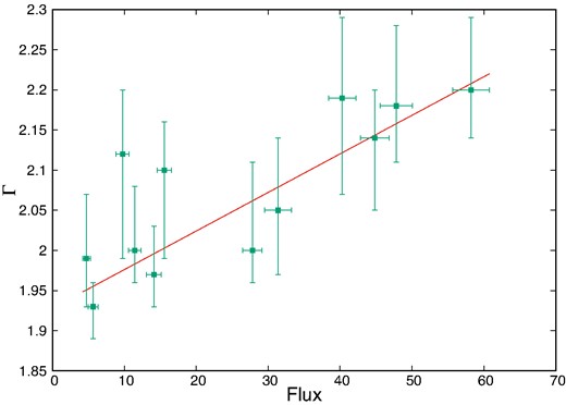
Variation of photon index (Γ) with 0.7–30 keV unabsorbed flux for the AstroSat data.
Considering the absorption-dominated scenario, we observed that the ionization parameter logξ for zxipcf the partial coverer ionized absorber was less compared to that of the reflection component xillverCp used to fit only the reflection component. Here we observed a highly ionized medium in the case of the reflection component, so its origin can be different from the ionized absorber. These results are consistent with results obtained by Ratheesh et al. (2021b), while analysing the similar low flux state NuSTAR data of GRS 1915 + 105 where they found that at all flux levels, the obscuring matter is highly ionized. We found that the ionization parameter for the ionized absorber varies between 1.97 and 3.14, with no clear trend of change with respect to flux, while as the hydrogen column density of the ionized absorber is anticorrelated with flux. We also observed a positive correlation between the normalization of the reflection component xillverCp and flux as evident from Table 2 (see Fig. 8).
We also observed that the flux calculated using absorption dominated model was greater than that of reflection dominated model. The reduced chi-square obtained during the fitting of data with reflection dominated model and ionized absorption model is plotted in Fig. 11, and we can see from the figure that both the models give similar statistical fits to the data. We have also verified this similar fit using the NuSTAR data, with parameters and the reduced chi-square obtained using both the models, presented in Tables 5 and 3. The reflection dominated interpretation is fairly similar to the reflection dominated spectrum used to model the low flux state of AGN. However, the spectra of GRS 1915 + 105 can also be interpreted as being due to high ionized absorption. Thus, unless different physical mechanisms are invoked for the similar spectra observed, it seems that either both type of sources in their low state, are either reflection dominated or highly absorbed. A comprehensive analysis using wide band data of both AGN and XRBs will reveal more information regarding the nature of these sources in their extreme low flux states.
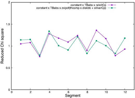
Comparison of reduced chi-square using different models.
5 CONCLUSIONS
We performed time resolved spectroscopy of a bright flare observed just a day after MAXI/GSC reported the re-brightening phase, during the anamolous low-flux state of GRS 1915 + 105, using broadband spectral capabilities of AstroSat. Our spectral fitting allowed for two different interpretations. In one interpretation source can be modelled as being relativistically blurred reflection dominated system and in the other interpretation having highly ionized absorber with high column densities. The two different interpretations of the spectra were confirmed by re-analysing a similar NuSTAR observation during the dim state of the source. For the absorption interpretation, the intrinsic flux of the source varied by a factor of ∼7 and hence the flare cannot be ascribed to a dramatic change in obscuration. Similarly for the reflection dominated model, the flare is due to intrinsic flux variation and the source remains reflection dominated throughout, indicating that the flare is not primarily due to any geometry changes.
We note that the relativistically blurred reflection dominated spectrum for a dim state of GRS 1915 + 105 is analogous to results obtained for AGN and hence the results presented here will have a bearing on AGN studies. Relativistically blurred reflection dominated spectra characterized by high reflection fraction has been observed in low flux state of many AGN (Seyferts) MCG-6-30-15, 1H 0707–495 (Fabian et al. 2004), and 1H0419-577 (Fabian et al. 2005). This enhanced reflection fraction in AGN is seen as a consequence of X-ray emitting source being very close to the central BH, and thus the light bending effects come into play. The low lamp-post heights and high reflection fraction in the spectra analyzed in this work, makes one of our spectral interpretation similar to the one used for the low flux state of AGN (Waddell et al. 2019; Barua et al. 2022). However, the spectra of GRS 1915 + 105 can also be interpreted in terms of high complex absorption and thus it may be that the low flux AGN spectra have a similar interpretation and more detailed studies are required.
ACKNOWLEDGEMENTS
We thank the anonymous reviewer for valuable and insightful comments. This publication uses the data from the AstroSat mission of the Indian Space Research Organisation (ISRO), archived at the Indian Space Science Data Centre (ISSDC). Data from LAXPC and SXT onboard AstroSat mission was used. We are thankful to LAXPC and SXT POC teams at TIFR Mumbai for providing the necessary software tools required for the analysis. SB is grateful to IUCAA Pune for regular visits under its visitor programme, where a part of this work was done. This research has made use of data and/or software provided by the High Energy Astrophysics Science Archive Research Center (HEASARC), which is a service of the Astrophysics Science Division at NASA/GSFC. SB thanks University Grants Commission (UGC), Govt. of India for providing fellowship under the UGC-JRF scheme (Ref. No.: 191620095661/CSIR-UGC NET DECEMBER 2019). VJ would like to acknowledge the Centre for Research Projects, CHRIST (Deemed to be University), for the financial support in the form of a Seed Money Grant (SMSS-2217).
DATA AVAILABILITY
The data utilized in this article are available at AstroSat-ISSDC website (http://astrobrowse.issdc.gov.in/astro archive/archive/Hom e.jsp) and NuSTAR Archive (https://heasarc.gsfc.nasa.gov/docs/nustar/ nustar archive.html). The software used for data analysis is available at HEASARC website (https://heasarc.gsfc.nasa.gov/lh easoft/download.html).
Footnotes
sxt_pc_mat_g0to4.rmf
SkyBkg_comb_EL3p5_Cl_Rd16p0_v01.pha
