


ABSTRACT
We present analysis on two X-ray bright points observed over several hours during the recent solar minimum (2020 February 21 and 2020 September 12–13) with the Nuclear Spectroscopic Telescope Array (NuSTAR), a sensitive hard X-ray imaging spectrometer. This is so far the most detailed study of bright points in hard X-rays, emission which can be used to search for faint hot and/or non-thermal sources. We investigate the bright points’ time evolution with NuSTAR, and in extreme ultraviolet (EUV) and soft X-rays with Solar Dynamic Observatory/Atmospheric Imaging Assembly (SDO/AIA) and Hinode/X-Ray Telescope. The variability in the X-ray and EUV time profiles is generally not well matched, with NuSTAR detecting spikes that do not appear in EUV. We find that, for the 2020 February bright point, the increased X-ray emission during these spikes is due to material heated to ∼ 4.2–4.4 MK (found from fitting the X-ray spectrum). The 2020 September bright point also shows spikes in the NuSTAR data with no corresponding EUV signature seen by SDO/AIA, though in this case, it was due to an increase in emission measure of material at ∼ 2.6 MK and not a significant temperature change. So, in both cases, the discrepancy is likely due to the different temperature sensitivity of the instruments, with the X-ray variability difficult to detect in EUV due to cooler ambient bright point emission dominating. No non-thermal emission is detected, so we determine upper limits finding that only a steep non-thermal component between 3 and 4 keV could provide the required heating whilst being consistent with a null detection in NuSTAR.
1 INTRODUCTION
When the full Sun is viewed in soft X-rays (SXRs), many small-scale bright points can be observed, distributed across the entire disc (Vaiana et al. 1973). These coronal bright points are small-scale bipolar loop structures located in the lower corona (e.g. Madjarska 2019) which are present throughout the solar cycle. They exist on average for less than a day, and are shorter lived in X-rays than in extreme ultraviolet (EUV), with lifetimes averaging at ∼ 12 h (Harvey et al. 1993), and they typically do not exceed temperatures of 2–3 MK (Doschek et al. 2010; Alexander, Del Zanna & Maclean 2011; Kariyappa et al. 2011). Throughout their lifetimes, bright points show variability in SXRs and EUV (Strong et al. 1992; Alexander et al. 2011), and many bright points are associated with dynamic phenomena, such as microflares (Kamio et al. 2011), jets (Shibata et al. 1992), and eruptions (Hong et al. 2014).
Coronal bright points are of particular interest due to their potential link to the problem of the unexplained high temperature of the solar corona. While large-scale heating events like flares do not produce the required heating, Parker (1988) proposed that the observed high temperatures could be a result of many tiny energy release events, termed nanoflares, too small to resolve individually. These nanoflare models predict high temperatures (> 5 MK) and/or non-thermal emission (Cargill 1994; Klimchuk 2015), and searching for these components requires higher energy X-ray observations.
HXR observations allow a search for such components as this emission would be dominated by the bremsstrahlung continuum from a thermal and/or non-thermal population of electrons. However, while bright points have previously been studied extensively in EUV and SXRs, there has been a lack of opportunity to do so in HXRs. Dedicated solar HXR instruments such as the Reuven–Ramaty High-Energy Solar Spectroscopic Imager (RHESSI; Lin et al. 2002) were designed to observe bright emission from flares and microflares, and were not optimized for observing faint small-scale sources like bright points. This meant that these features could not be individually observed, though upper limits have been obtained on the HXR emission from the full quiet Sun using data from RHESSI (Hannah et al. 2007, 2010), and more recently from the Focusing Optics X-Ray Solar Imager sounding rocket (Buitrago-Casas et al. 2022).
The Nuclear Spectroscopic Telescope Array (NuSTAR; Harrison et al. 2013) is a highly sensitive focusing HXR telescope that observes at ∼ 2–79 keV. NuSTAR is an astrophysics mission, but is also capable of being pointed at the Sun (Grefenstette et al. 2016), allowing the observation of small-scale solar sources such as X-ray bright points. There have been a number of NuSTAR solar observing campaigns, with much of the analysis focusing on active region microflares (Glesener et al. 2017; Wright et al. 2017; Hannah et al. 2019; Cooper et al. 2020; Glesener et al. 2020; Cooper et al. 2021; Duncan et al. 2021), and also on smaller transient brightenings in the quiet Sun (Kuhar et al. 2018), finding hotter and non-thermal sources existing in considerably smaller microflares than previously studied.
The recent solar minimum (2018–2020) provided a unique opportunity for sensitive HXR observations of small-scale sources in the quiet Sun with NuSTAR. During this period, there were several solar observing campaigns, and work on one of these observations (from 2018 September 28) was presented in Paterson et al. (2023). This study analysed NuSTAR data for a number of quiet Sun features, including several X-ray bright points. From NuSTAR HXR spectroscopy and differential emission measure (DEM) analysis, it was found that these features did not reach temperatures above 3.2 MK, and no non-thermal emission was observed. However, this NuSTAR observation was done in the full-disc mosaic mode, changing pointing every ∼ 100 s over the course of an hour. Therefore, the time evolution of the bright points in HXRs could not be thoroughly investigated, and the data were noisy due to short pointing times.
In addition to several mosaics, there are also NuSTAR dwell observations of the quiet Sun from the recent minimum. For these, NuSTAR’s pointing remained constant throughout each NuSTAR orbit (with ∼ 1 h in sunlight), allowing for a more rigorous analysis of the temporal evolution of any sources present. In this paper, we present analysis on X-ray bright points observed in NuSTAR solar dwell observations from 2020 February 21 and September 12–13.
The role of bright points in the overall context of the solar atmosphere and solar activity, and their relationship to active regions, remains poorly understood. In order to improve our understanding of these features and their contribution to heating the solar atmosphere, we investigate the variability of the two bright points throughout hours of data, searching for the presence of high-temperature (> 5 MK) or non-thermal emission. We also study their evolution in EUV and SXRs, making use of data from Solar Dynamic Observatory’s Atmospheric Imaging Assembly (AIA; Lemen et al. 2012) and the Hinode X-Ray Telescope (XRT; Kosugi et al. 2007).
A brief overview of the NuSTAR observations is detailed in Section 2. Analysis, including NuSTAR spectral fitting and DEM analysis, of an X-ray bright point from the 2020 February 21 observation is presented in Section 3. Analysis of a second bright point observed on 2020 September 12–13 can be found in Section 4. Section 5 discusses the results, including discrepancies found between the EUV and HXR time profiles of the bright points, which point to substantial shortfalls in standard models of flaring loops.
2 OVERVIEW OF OBSERVATIONS
On 2020 February 21, NuSTAR observed the quiet Sun for 11 orbits in total, with the first beginning just after 05:15 ut and the observation ending at around 22:20 ut. Of these 11 orbits, 2 (the second and second-to-last) were observed in full-disc mosaic mode, and the other 9 in dwell mode (NuSTAR observation IDs 80512218001–80512228001). During these dwell orbits NuSTAR was pointed at disc centre, capturing a field of view (FOV) of 12 × 12 arcmin2. As the Sun was relatively quiet, the NuSTAR livetime (the fraction of time during which NuSTAR is able to detect incoming photons) for this observation was 47–93 per cent, considerably higher than that for NuSTAR active region and microflare studies (for instance, 0.1 per cent for a microflare in Glesener et al. 2020). There were a number of bright points observed throughout the NuSTAR orbits, the largest of which was present for the full observation and so is ideal for studying time evolution. This bright point is summarized in the top row of Fig. 1.
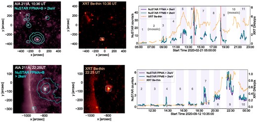
A summary of the bright points captured with NuSTAR on 2020 February 21 (top panel) and 2020 September 12–13 (bottom panel). Left panel: AIA 211 Å image, showing the region that NuSTAR captured, with aligned NuSTAR contours summed over its two focal plane modules (FPMA and B) shown in blue (at 3, 8, and 50 × 10−3 count s−1 in the top left panel and at 1, 5, and 20 × 10−3 count s−1 in the bottom left panel). Centre panel: XRT Be-thin image of the same region. Right panel: NuSTAR FPMA (purple) and FPMB (blue), and XRT Be-thin (orange) time profiles for the bright points, calculated over the white box indicated on the XRT image (which was appropriately shifted to account for the Sun’s rotation). The shaded areas highlight the times of the orbits where NuSTAR was observing in dwell mode, and the orbit numbers are indicated in grey (note that only orbits 2–10 are shown for the 2020 September observation since the first orbit was a mosaic). The red-dashed lines on the top right panel highlight the times of the flares analysed for the 2020 February bright point. The two large spikes in the earlier orbits in the NuSTAR time profiles for the 2020 September bright point are due to ghost rays from sources outside the FOV.
This figure shows an AIA 211 Å and an XRT image of the disc centre region that NuSTAR observed. These are overplotted with NuSTAR contours summed over its two identical telescopes, FPMA and FPMB, which each have an angular resolution of 18 arcsec and detectors with 0.6-mm pixels. NuSTAR has a pointing uncertainty of ∼1.5 arcmin during solar observations (Grefenstette et al. 2016), meaning that its images must be aligned with an image from an instrument with a better pointing accuracy. The NuSTAR contours were aligned with the AIA 211 Å images by shifting the NuSTAR images such that the brightest features lay on top of their counterparts in AIA. Convincing agreement between the two instruments is demonstrated in the co-aligned image in Fig. 1, top left panel.
In this image, several bright points are apparent in AIA. While some of these small bright points were captured with NuSTAR as well as AIA, the brightest source is the larger bright point just below disc centre at ∼ (–50 arcsec, –300 arcsec). This source is present throughout all of the NuSTAR orbits. Though not bright enough to be given a NOAA identification, this feature was detected with the Spatial Possibilistic Clustering Algorithm (Verbeeck et al. 2014) as SPoCA 23914. This NuSTAR bright point had a lifetime of ∼4 d, longer than that of typical X-ray bright points, which generally have lifetimes < 48 h (Golub, Krieger & Vaiana 1976). While this longer lifetime does lead to some ambiguity as to the nature of this source, here we consider this feature to be an X-ray bright point as opposed to a small active region.
NuSTAR and XRT time profiles for this bright point are shown in the top right panel. Note that the largest gaps in the NuSTAR data are when the two full-disc mosaics were being taken, at 06:54–07:53 and 19:46–20:46 ut. It can be seen that the X-ray emission from this source shows significant variability over the course of the observation, with the NuSTAR and XRT time profiles exhibiting broadly similar behaviour. Until around 11:00 ut, the source is relatively quiet in both instruments, after which the X-ray emission begins to increase, leading to a number of peaks.
On 2020 September 12–13, NuSTAR observed the Sun for 10 orbits, with livetimes between 86 and 92 per cent. The first of these orbits was observed in full-disc mosaic mode, beginning just after 09:00ut on September 12. The following 9 orbits (NuSTAR observation IDs 80 600 201 001 and 80610202001–80610210001) were all observed in dwell mode, with the final orbit concluding at 00:35 ut the next day. While the 2020 February 21 dwell orbits focused on disc centre, in this observation NuSTAR was pointed at a region on the East limb. At this time, there were few steady sources present in this region (though there were several small transient brightenings), but an X-ray bright point emerged later on in the observation.
A summary of this bright point is shown in the bottom row of Fig. 1. This feature lies close to the East limb, at ∼ (–800 arcsec, –50 arcsec), as shown in the AIA 211 Å and XRT images. It can be seen from the X-ray light curves (bottom right panel) that this feature was captured by NuSTAR only in the final three orbits (orbits 8–10). The XRT light curve begins to show this bright point’s emergence at around 19:30 ut. In both NuSTAR and XRT, the bright point is brightest in orbit 9 (in which there are several spikes in the X-ray time profiles), after which the brightness decays through to orbit 10. Note that the two NuSTAR spikes apparent in earlier orbits are due to ghost rays (Grefenstette et al. 2016) from sources outside NuSTAR’s FOV. At the time of both peaks, the NuSTAR images (not shown) exhibit the distinct radial pattern that is associated with ghost rays (Madsen et al. 2015).
Analysis on the bright points from 2020 February and September can be found in Sections 3 and 4, respectively. These particular data sets were chosen for this analysis due to them having many orbits worth of data, in addition to them both being from times when the Sun was very quiet (no active regions on disc, GOES/XRS flux below A-level, etc.). As a result, analysis of the bright points’ evolution could be performed over many hours, with increased chance of detecting any high-temperature or non-thermal emission present. For both of these observations, there is also data available from AIA and XRT, meaning that the bright points’ evolution in EUV and SXRs could also be investigated.
3 THE LARGEST BRIGHT POINT IN THE 2020 FEBRUARY 21 OBSERVATION
The X-ray time profiles for the largest bright point in the 2020 February 21 observation (shown Fig. 1, top right) exhibit several spikes, where the source is ‘flaring’. Though there are several times where the NuSTAR light curve shows interesting behaviour, in this paper, we focus only on the two largest flares in NuSTAR, the first occurring just before 14:00 ut in orbit 6 (the brightest) and the second at around 18:15 ut in orbit 9. These events are highlighted by red-dashed lines on the time profiles in Fig. 1. Analysis on these two events can be found in the following subsections (Sections 3.1 and 3.2, respectively).
3.1 Flare 1
The brightest of the 2020 February 21 NuSTAR peaks was captured in orbit 6 (13:20–14:20 ut). It can be seen from the time profile for the bright point over all orbits in Fig. 1 that the source is relatively faint in NuSTAR at the beginning of this orbit. There is a data gap from 13:35–13:49 ut, after which the NuSTAR light curve has more than doubled. This increase in NuSTAR continues, reaching a peak at around 13:55 ut. Around this time, there is also a peak in the XRT Be-thin time profile.
Fig. 2 details the evolution of this event in EUV with AIA and X-rays with XRT and NuSTAR. The top right panel contains AIA images showing the evolution of this event, overplotted with NuSTAR contours, and the bottom panel shows XRT images. The NuSTAR contours were aligned with the AIA images so that the bright centre of the NuSTAR emission lay on top of the brightest region in AIA 211 Å. It can be seen from the AIA images that at the time of the NuSTAR event, there is a brightening in a region near the bottom of the bright point. Time profiles for this event are shown also in this figure, in the top left panel. For AIA, a region around the resolved brightening source was used, but given their spatial resolution, the whole bright point region had to be used instead for XRT and NuSTAR. Using this full region for AIA, the brightening would be harder to spot, as the time profile would be dominated by the EUV emission from the rest of the bright point. It can be seen that the XRT Be-thin and Al-poly time profiles show increased emission the same time as NuSTAR, though they reach a peak slightly later. This is because XRT was observing with a cadence of 6 min, and unfortunately missed the exact time of the NuSTAR peak. Note that NuSTAR’s spatial resolution means that some of the point spread function (PSF) falls outside of the region used to calculate the light curves. However, this is not a problem because the time profiles show the correct relative flux, and the PSF is taken into account for spectroscopy.
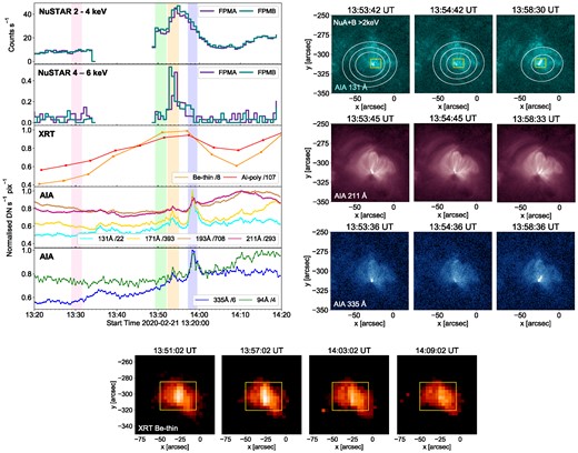
Top left panel: NuSTAR, XRT, and AIA time profiles for the flare in orbit 6 on 2020 February 21. The maximum values, which were used to normalize the AIA and XRT time profiles, are indicated on the legends. Shaded regions show time ranges used for spectral analysis. Top right panel: AIA 131, 211, and 335 Å panels showing the EUV evolution of the event. The AIA 131 Å images on the top row are overplotted with NuSTAR FPMA + B > 2 keV, with contours at 0.04, 0.06, and 0.08 count s−1. The yellow boxes show the region that the AIA time profiles were calculated over. Bottom panel: XRT Be-thin images showing the SXR evolution of the event, with the yellow boxes showing the region that the XRT and NuSTAR time profiles were calculated over.
Unlike the X-ray time profiles, AIA sees two distinct peaks. The first AIA peak coincides with the brightening that NuSTAR detects, with the peak occurring at the same time as the peak in the NuSTAR 4–6-keV energy band (∼ 13:53:40 ut) and the rise in the 2–4-keV band. This first peak is followed by a minimum in AIA, and then the time profiles for all AIA channels rise to a second higher peak at 13:58:30 ut. During the first NuSTAR peak, there is clearly increased EUV emission and when there is a minimum in the AIA time profile, there is no evidence of any brightenings in the AIA images.
During the time of the second AIA peak, it can be seen that there is EUV emission extending along a loop, originating from the area that brightened originally. The NuSTAR time profile indicates that the HXR emission is still elevated but decreased from the first peak. This discrepancy between the HXR and EUV time profiles suggests that AIA and NuSTAR are seeing emission from different temperatures at this time, with the brightening occurring at temperatures below NuSTAR’s sensitivity. Different regions were used to calculate the AIA and NuSTAR time profiles (the region used for NuSTAR covered the whole bright point, but only the brightening region was used for AIA). However, using the same larger region to calculate the AIA light curve did not make the EUV and X-ray profiles more similar, and only made the peaks less prominent.
3.1.1 NuSTAR spectral analysis
NuSTAR is an imaging spectrometer, and therefore we fitted the bright points’ HXR spectra to investigate their properties. Here, we do this for chosen time ranges over circular regions enclosing the source. To fit the spectra, we made use of XSPEC (Arnaud 1996), an X-ray spectral fitting program. With XSPEC, the FPMA and FPMB spectra can be fitted simultaneously to improve the signal-to-noise, introducing a constant multiplicative factor (which is a fit parameter for FPMB) to account for any systematic differences between the two detectors. Note that these spectra were fitted down to energies of 2.2 keV, rather than the previously recommended 2.5 keV (Grefenstette et al. 2016), which was possible due to a recent update to NuSTAR’s calibration (Madsen et al. 2022). This helps to improve the fits as these weak events are predominantly at lower X-ray energies.
For this event, we chose several time ranges (shown as shaded regions on the time profiles in Fig. 2) to perform spectral analysis for: a quiescent time from 13:29:00–13:31:30 ut (pink); an early flare time from 13:49:20–13:52:00 ut (green), during which the NuSTAR time profile is relatively flat just prior to the sharp increase in emission; a flare time from 13:52:20–13:55:00 ut (orange), which covers the rise time; and the time of the AIA peak from 13:57:20–13:59:30 ut (blue), which occurs during NuSTAR’s gradual phase. The flare time was chosen to be the interval during which increased emission was detected in the NuSTAR 4–6-keV energy range. By selecting a time range where the higher energy emission is peaking, the chances of detecting a high-temperature or non-thermal component in the spectral fitting are increased.
The top row of Fig. 3 shows the NuSTAR HXR spectra for the bright point for all four times, fitted with isothermal models. It can be seen that during the intial quiescent time, an isothermal model with a temperature and emission measure of 3.28 MK and 1.60 × 1044 cm−3 fits the NuSTAR spectrum adequately. During the early flare time, the observed spectrum is well fitted with an isothermal model with a temperature and emission measure of 3.22 MK and 5.35 × 1044 cm−3, respectively. For the flare time, the fitting results in a higher temperature of 3.46 MK and an emission measure of 4.53 × 1044 cm−3. However, unlike for the early flare time, this spectrum is not adequately fitted with this isothermal model. There is an excess in the data compared to the model above 4 keV. This is indicative of the presence of a hotter (or potentially non-thermal) component.
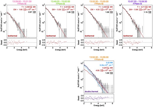
Top row: from left to right panels, NuSTAR FPMA + FPMB spectra for the 2020 February 21 bright point for Flare 1. The spectra are for the quiescent time (13:29:00–13:31:30 ut), the early flare time (13:49:20–13:52:00 ut), the flare time (13:52:20–13:55:00 ut), and the time of the AIA peak (13:57:20–13:58:30 ut), fitted with isothermal models (red). Bottom panel: NuSTAR FPMA + FPMB spectrum from the flare time, fitted with a double thermal model (purple; separate thermal components shown in blue and red). Dashed lines indicate fitting range, the lower panels show the residuals, and temperatures and emission measures (and the multiplicative constant) are marked on plots.
As the isothermal model is not sufficient to deal with the flare time spectrum, we also fitted this spectrum with a double thermal model. The early flare time isothermal model (with T = 3.22 MK and EM = 5.35 × 1044 cm−3) was set as a fixed background component in the fitting. When fitted, it was found that the resulting second thermal model had a temperature of 4.24 MK and an emission measure of 4.85 × 1043 cm−3, as shown in the bottom panel of Fig. 3. Fitting this spectrum with a double thermal model was found to produce a lower c-stat fit statistic in comparison to the isothermal fit. It can also be seen in Fig. 3 that the residuals are smaller at higher energies with the double thermal model.
When the spectra from the early flare and flare times are fitted with isothermal models, the drop in emission measure that coincides with the increase in temperature is due to NuSTAR being sensitive to the hottest material present (and so the isothermal fit results from the flare time are a reflection of the hotter, fainter emission present during this time). The decrease in emission measure during an HXR spike indicated by the isothermal fits is therefore slightly misleading, and is really indicating that the double thermal interpretation, wherein the early flare time spectrum is taken to be a fixed component, is a more physically realistic model. However, DEM analysis is required in order to fully understand the multithermal evolution of this event (see Section 3.1.2).
The double thermal interpretation suggests that there is material with temperatures higher than 4 MK in this feature during the flare time. It can be seen that, even with this double thermal model, there is still a small excess at higher energies, which we will investigate further in Section 3.1.3.
The spectrum from the time of the AIA peak (during NuSTAR’s gradual phase) is well fitted with an isothermal model. This fit gives a temperature of 3.21 MK, the same as the temperature during the early flare time. However, the emission measure is higher during this time interval, at 5.99 × 1044 cm−3, reflecting the behaviour of the time profile in Fig. 2. There is no indication of a hotter component at this time.
3.1.2 Differential emission measures
In order to examine the different behaviour of the X-ray and EUV time profiles for this event, we reconstructed DEMs for this bright point for several different times. This allowed us to investigate the changes in the multithermal properties of this source during the times where NuSTAR, XRT, and AIA are all peaking, and where only AIA peaks. Here, the DEMs were reconstructed using the regularized inversion approach detailed in Hannah & Kontar (2012), using data from the six AIA coronal temperature channels and NuSTAR, splitting the NuSTAR data into the two energy bands 2.2–3.6 and 3.6–6.0 keV. Systematic uncertainties of 20 per cent were assigned to each of the data values. The photon shot noise was insignificant in comparison to this systematic uncertainty for the AIA channels. However, the photon noise was larger for NuSTAR, and so was added in quadrature with the systematic uncertainty. The AIA data were averaged over all of the images in the chosen time ranges. The AIA version 10 responses were calculated using CHIANTI version 9.3 (which was also used in calculating the NuSTAR and XRT responses).
We reconstructed the DEM for three of the time ranges previously used for spectroscopy: the quiescent time before the NuSTAR data gap; the flare time, where a peak was observed with both NuSTAR and AIA; and the second peak, observed only with AIA during NuSTAR’s gradual phase. We calculated the DEMs over the same area used to obtain the time profiles shown in Fig. 2. This was the brightest region in AIA even before the flare, and it was therefore assumed that the majority of the NuSTAR emission originated from this region. Note that XRT data were not used here as there was not an XRT image corresponding to each of the time ranges.
Fig. 4 shows the DEMs for this region during the chosen time intervals. It can immediately be seen that these DEMs show a two-peak structure, with peaks at log(T) = 5.7 and log(T) = 6.3, and that all three are very similar for log(T) < 6.3. At temperatures higher than this, the DEM from the quiet time falls off much more sharply.
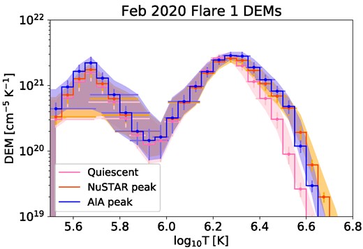
DEMs for Flare 1 on 2020 February 21 calculated using NuSTAR and AIA data from the following times: 13:29:00–13:31:30 (pink), 13:52:20–13:55:00 (orange), and 13:57:20–13:59:30 ut (blue). These time ranges are highlighted on the time profiles in Fig. 2.
The two DEMs from the flare time only show differences at higher temperatures. Up to log(T) ∼ 6.6, these two DEMs are very similar, but the DEM from the time of the NuSTAR peak is the higher of the two at temperatures above this. This is the time range corresponding to the peak in the NuSTAR 4–6-keV band, where the NuSTAR spectral analysis indicated increased emission at ∼ 4.2 MK. The DEM obtained here confirms these results.
The DEM for the time range where AIA peaks but NuSTAR does not falls off more sharply than for the time of the first peak, suggesting that less high-temperature emission is present. However, this DEM is the higher of the two for 6.3 < log(T) < 6.5, indicating that this brightening takes place at cooler temperatures (2–3 MK) than the first peak. Therefore, this suggests that this brightening occurred due to the material cooling into a temperature range where AIA has more sensitivity but NuSTAR still has some, and so appears as a gradual phase in NuSTAR but a peak in AIA. However, as these two DEMs are not different from each other at these temperatures when the error bars are taken into account, this result is not conclusive.
3.1.3 Non-thermal upper limits
There is a small excess in the double thermal fit for this event, as shown in the spectrum in Fig. 3 (bottom panel). We attempted to fit an additional non-thermal component to this spectrum, but could not obtain a reliable fit. Instead, we used the observed number of counts at higher energies to determine upper limits on the non-thermal emission that could have been present following the approach used by Wright et al. (2017) and Paterson et al. (2023) (see these papers for full details). A non-thermal component was added to a spectrum simulated from the double thermal model which was fitted to the observed spectrum (bottom panel of Fig. 3). There is an excess of 10 counts between 5 and 6 keV in the observed counts compared to the model, so any additional non-thermal component should not produce any more counts than this at these energies. The three parameters defining the non-thermal model were the power-law index, the low energy cutoff, and the electron flux. For several combinations of power-law index and low energy cutoff, the electron flux was reduced until the non-thermal component was smaller than the photon noise at energies < 5 keV, and the counts between 5 and 6 keV did not exceed 10 |$\pm \sqrt{10}$|. The non-thermal power for the resulting model was then taken to be the upper limit.
This non-thermal power can be compared with the thermal energy of the event in order to determine whether the heating could have been via accelerated electrons. The thermal energy can be calculated by
where kB is the Boltzmann constant, T and EM are the temperature and emission measures of the emitting plasma, respectively, and V is the corresponding volume, taken here to be A3/2, where A is the area of the source in AIA. This energy is then divided by the duration of the event to obtain a thermal heating requirement. If this requirement is less than the non-thermal upper limit, then the heating could be non-thermal.
For this event, the emitting area was taken to be a smaller region (5 × 5 arcsec2), of just the brightening region, not the box used to calculate the time profiles. Using the temperature and emission measure from the hotter component in the double thermal fit (T = 4.24 MK, EM = 4.85 × 1043 cm−3), it was found that the thermal energy of this brightening was 8.47 × 1025 erg. This can be divided by the observation time of 160 s to obtain a required heating power of 5.30 × 10²³ erg s−1.
It was found that there was a small range of parameters for which the non-thermal model chosen could produce the required heating. In order for the calculated non-thermal upper limits to be consistent with this heating requirement, the non-thermal distribution would have to be very steep (with a power-law index ≥ 7), with a low energy cutoff between 3 and 4 keV.
A larger region, with an area in AIA of 13 × 11 arcsec2 (indicated in Fig. 2, top left), was used to calculate DEMs and light curves for this event. This region enclosed the more extended brightening which was observed during the second AIA peak at 13:57:20–13:59:30 ut. For calculating the non-thermal upper limits during the time of the strongest NuSTAR emission, we used only the smaller region which showed increased brightness in AIA at this time, with area 5 × 5 arcsec2. We found that using the larger area increased the thermal energy estimate for the event and therefore also increased the heating requirement, which only a monoenergetic non-thermal electron distribution with a low energy cutoff at ∼ 3 keV (which seems physically implausible) could satisfy.
3.2 Flare 2
The second brightest peak in the NuSTAR time profile occurs around 18:15 ut, shortly after the beginning of the ninth NuSTAR orbit. Unfortunately, there is a gap in the XRT data between 18:05 and 18:35 ut, meaning that it did not capture this event. However, the XRT brightness does increase from around 17:00 ut (the same time that the NuSTAR time profile begins to rise), reaching a maximum on the final image before the data gap. After the data gap, the XRT emission has decreased.
The left-hand panel of Fig. 5 shows the time profiles for this event for NuSTAR, as well as for AIA. It can be seen that the NuSTAR time profile is flat for several minutes after the orbit begins at ∼ 18:10 ut. The emission begins to increase at 18:12 ut, and reaches a peak at 18:14 ut. However, though NuSTAR detects a clear rise in emission, the AIA light curves show no clear signature for this event, just a steady increase in brightness across all channels. These light curves were calculated over a box enclosing the full bright point (indicated on the AIA 131 Å images in Fig. 5). However, AIA light curves were also obtained for smaller regions across the source, and none showed clear evidence of increased emission at the time of the NuSTAR event.
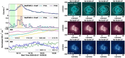
Left panel: NuSTAR 2–4 and 4–6 keV and AIA time profiles for the flare in orbit 9 on 2020 February 21. The maximum values, which were used to normalize the AIA time profiles, are indicated on the legends. The coloured regions indicate time ranges used for spectral analysis, shown in Fig. 6. Right panel: AIA 131, 211, and 335 Å images showing the EUV evolution of this event. White contours are NuSTAR FPMA + B > 2 keV (plotted at 0.01, 0.02, and 0.03 count s−1), and the yellow box shows the region used for calculating the light curves.
The AIA images from the time of the NuSTAR flare (shown in the right-hand panel of Fig. 5) also show no obvious changes in brightness. This lack of detection in AIA could be explained by NuSTAR seeing tiny increases in brightness which, in EUV, are too small compared to the dominant emission at 2–3 MK to be observed. Not having the XRT data means that this event cannot be confirmed with another instrument. However, this brightening in the NuSTAR data does not appear to be caused by the source moving in and out of detector gaps, and there were no NuSTAR pointing shifts around this time, suggesting it is real. Also, this event cannot be attributed to ghost rays as it appears as a distinct imaged source in the NuSTAR image, rather than an easily identifiable radial ghost ray pattern.
3.2.1 NuSTAR spectral analysis
Two time ranges were chosen to fit the NuSTAR spectra over. At the start of orbit 9, there is a small time interval where the NuSTAR time profile is flat, from 18:09:30–18:11:40 ut. This time range, marked on the NuSTAR time profiles in the left-hand panel of Fig. 5, was taken to be the pre-flare time. Again, the flare time was chosen to correspond to the time of increased emission in the 4–6-keV light curve (18:12:30–18:14:50 ut), also shown in this figure.
The NuSTAR spectra for these time ranges were both fitted with isothermal models, and the results of this are plotted in the two left-hand panels of Fig. 6. For the pre-flare time, the spectrum is well fitted with an isothermal model with a temperature of 3.20 MK and an emission measure of 5.89 × 1044 cm−3. The isothermal model fit to the spectrum from the flare time has a higher temperature of 4.01 MK and an emission measure of 2.85 × 1044 cm−3. Similarly to the previous event, the flare time spectrum shows an excess compared to the model at higher energies, indicating that the thermal model alone is not sufficient to fit this spectrum.
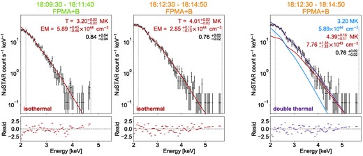
Left panel: NuSTAR FPMA + FPMB spectra for the 2020 February 21 bright point for Flare 2. The spectra are for the pre-flare (18:09:30–18:11:40 ut) and flare (18:12:30–18:14:50 ut) times, fitted with an isothermal model (red). Right panel: NuSTAR FPMA + FPMB spectrum from the flare time, fitted with a double thermal model (purple; separate thermal components shown in blue and red). Dashed lines indicate fitting range, the lower panels show the residuals, and temperatures and emission measures (and the multiplicative constant) are marked on plots.
Therefore, the flare time spectrum was also fitted with a double thermal model, where the first component was fixed to be the isothermal model which was fitted to the pre-flare spectrum. The results of this fitting are also shown in Fig. 6 (right panel). It was found that the second thermal component required to fit this spectrum had a temperature and emission measure of 4.39 MK and 7.76 × 1043 cm−3. Fitting the NuSTAR spectrum from the flaring time with this double thermal model produced a lower c-stat fit statistic than fitting with the isothermal model, and resulted in smaller residuals at higher energies. As was the case with Flare 1, the double thermal fit to the flare time spectrum presents a more physically realistic model for the X-ray brightening.
3.3 Non-thermal upper limits
Non-thermal upper limits were calculated for this event and compared with the heating requirement from its thermal energy using the same method detailed in Section 3.1.3. However, since this event was not clearly detected with AIA, it is difficult to accurately select the area of the source when calculating the thermal energy. Therefore, the calculated non-thermal upper limits were compared to the thermal heating requirement calculated using several different areas: the area of a single AIA pixel (0.6 × 0.6 arcsec2), the area used for the previous event (5 × 5 arcsec2), and an area covering the entire bright point (35 × 35 arcsec2).
Taking the temperature and emission measure from the hotter thermal component during the event time (T = 4.39 MK, EM = 7.76 × 1043 cm−3), the thermal energy was calculated for these three areas. The resulting thermal energies were found to be (from smallest to largest area) 4.61 × 1024, 1.11 × 1026, and 2.05 × 1027 erg.
Fig. 7 shows the thermal heating requirements from these energies (calculated by dividing the thermal energy by the event duration of 140 s), and the non-thermal upper limits obtained from the NuSTAR spectrum. This plot highlights the effect that changing the area has on the conclusion as to whether the heating could be non-thermal. Using the area of one AIA pixel, a non-thermal component with a low energy cutoff up to ∼5 keV and a power-law index ≥ 7 could provide the necessary heating, whereas using an area covering the whole bright point results in no possible combinations that satisfy the requirement. When a more realistic example is chosen (here using the area from the previous event), a steep non-thermal distribution between 3 and 4 keV could provide the required heating. However, with any increased emission in AIA being undetectable, it is not possible to make a definitive conclusion.
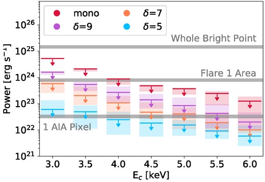
Non-thermal upper limits for Flare 2 on 2020 February 21 for a range of low-energy cutoffs (Ec) and power-law indices (δ = 5, 7, 9, and monoenergetic with E = Ec). The grey-shaded regions are the heating requirements determined by the thermal energy for different areas.
4 THE BRIGHT POINT IN THE 2020 SEPTEMBER 12–13 OBSERVATION
On 2020 September 12–13, the bright point that NuSTAR observed only emerged towards the end of the observation. The NuSTAR, XRT, and AIA time profiles over the last three NuSTAR orbits only are shown in the right-hand panel of Fig. 8. It can be seen that the NuSTAR and XRT Be-thin light curves show a similar pattern. For both, the middle orbit (orbit 9) is the one with the strongest emission and the most variability. There are three peaks in the NuSTAR time profile during this orbit, which are also observed in XRT Be-thin. As seen in the XRT images and NuSTAR contours, the time of brightest X-ray emission is between 22:03–22:23 ut. In orbits 8 and 10, the HXR and SXR emission is fainter, with much less variability. Though the NuSTAR and XRT time profiles are in good agreement, the EUV evolution does not follow the same trend. Over the course of the three orbits, the bright point continually increases in brightness in all AIA channels, reaching a plateau at around 23:00 ut. This bright point is brightest in EUV in orbit 10, at which point it has faded in X-rays compared to the previous orbit. Also, in orbit 8, the AIA time profiles show no evidence of the spikes that appear in the NuSTAR light curve. AIA time profiles were made for smaller regions within the bright point, but no similar behaviour to NuSTAR could be clearly identified.
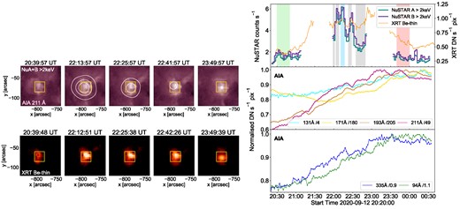
Left panel: AIA 211 Å (top panel) and XRT Be-thin (bottom panel) images showing the temporal evolution of the bright point from the 2020 September 12 observation, over the final three NuSTAR orbits. The first image is from orbit 8, the middle three from orbit 9, and the last from orbit 10. The white contours are NuSTAR FPMA + B > 2 keV (plotted at 5, 8, and 10 × 10−3 count s−1). The yellow box indicates the region that time profiles were calculated over. Right panel: NuSTAR, XRT, and AIA time profiles for the bright point for the last three NuSTAR orbits. The maximum values, which were used to normalize the AIA time profiles, are indicated on the legends. Shaded regions show time ranges chosen for spectral analysis, with the coloured time ranges also being used to calculate the DEMs shown in Fig. 10.
4.1 NuSTAR spectral analysis
Having NuSTAR HXR data for several hours of this bright point’s evolution gives the opportunity to perform spectral analysis to investigate how its properties change over time. For this analysis, several time intervals over the three orbits were chosen, shown as shaded regions on the time profile plot in Fig. 8. In orbit 8, the NuSTAR emission is reasonably constant, so a broad time range from 20:30–20:50 ut was chosen in order to get the best signal-to-noise. In orbit 9, where the NuSTAR emission is more variable, five separate time ranges were used: 21:58:50–22:01:30 ut (a brief time where the time profile is relatively flat), 22:03:30–22:08:00 ut (the first NuSTAR peak), 22:11–22:17 ut (the second and brightest NuSTAR peak), 22:23–22:28 ut (a smaller third peak), and 22:35–22:50 ut (where there is a minimum in the NuSTAR emission). By orbit 10, the brightness in NuSTAR has reduced to a lower, and relatively constant, level and so a longer time range from 23:40–00:00 ut was used.
The results of fitting the NuSTAR spectra from these seven time ranges with isothermal models are summarized in Fig. 9. It was found that the NuSTAR fit temperature for this feature stayed roughly constant at ∼ 2.6 MK throughout the three orbits. The fits from all time ranges produced this temperature, except for 22:35–22:50 ut, where there was a minimum in the NuSTAR light curve after the peaks. This spectrum was fitted with an isothermal model with a slightly cooler temperature of 2.44 MK (and an emission measure of 3.03 × 1044 cm−3).
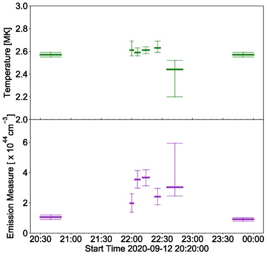
Plots of temperature (top panel) and emission measure (bottom panel) against time for the 2020 September bright point. These were obtained by fitting the NuSTAR spectra over the time ranges indicated in Fig. 8 with isothermal models.
For the other times, the emission measure was lowest during orbits 8 and 10, at ∼ 1 × 1044 cm−3. At these two times, the NuSTAR time profile is at around the same level, which is lower than during orbit 9. From the start of orbit 9, throughout the three peaks, the NuSTAR fit temperature stays constant at 2.6 MK while the emission measure varies. The emission measure increases from 1.97 to 3.54 × 1044 cm−3 between the start of the orbit and the first peak. The emission measure is at its highest during the middle peak (the largest one) at 3.66 × 1044 cm−3, and is slightly lower during the third peak at 2.41 × 1044 cm−3.
The fact that the NuSTAR fit temperature remains approximately constant while the emission measure changes indicates that the brightening of this feature in orbit 9 is due to an increase in the amount of emitting material, as opposed to an increase in temperature in the emitting material.
Most of these spectra are adequately fitted with the isothermal models, and show no evidence of higher temperature or non-thermal components. However, the spectra from the two strongest NuSTAR peaks in orbit 9 do show a small excess at higher energies, indicating the presence of hotter or non-thermal emission. However, the excesses do not appear to be significant, which can be confirmed via DEM analysis.
4.2 Differential emission measures
As well as spectral analysis, we also investigated the evolution of this feature through the change in its DEM. We calculated the DEM for this feature (using the same method detailed in Section 3.1.2) for three separate times, which were also used for the spectral fitting in the previous section: the quiet time in orbit 8 (20:30–20:50 ut); the time of the largest peak in orbit 9 (22:11–22:17 ut); and the time of decreased X-ray but increased EUV emission in orbit 10 (23:40–00:00 ut). As XRT data were available at these times, it was included in the DEM calculation. The XRT response was multiplied by a factor of two following the approach of Wright et al. (2017) and Paterson et al. (2023), where including this factor was found to produce smaller residuals (which was also found to be the case here).
The DEMs calculated for the three chosen time ranges are shown in Fig. 10. The DEM during orbit 10 is higher than that for orbit 8 for 5.8 < log(T) < 6.3. This is consistent with the increase in EUV emission between these two times observed in all six of the AIA channels, seen in the time profiles in Fig. 8. At log(T) > 6.3, the two DEMs are very similar as they fall off. Again, this is in agreement with the X-ray time profiles being at similar levels during these times.
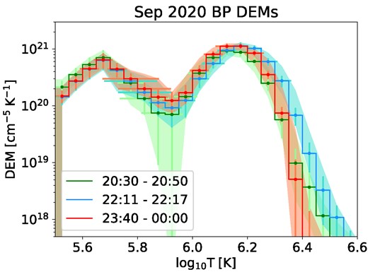
DEMs of the September bright point from orbit 8 20:30–20:50 ut (green), orbit 9 22:11–22:17 ut (blue), and orbit 10 23:40–00:00 ut (red). These time ranges are shaded on the time profile in Fig. 8.
The DEM from the largest peak (during orbit 9) is similar to the other two DEMs at log(T) < 6.2. However, at higher temperatures, this DEM shows a larger amount of material than at the two other times. This is consistent with orbit 9 being the time of peak emission in X-rays, suggesting the presence of more material > 2.5 MK, but there is little significant emission above 3 MK. All three DEMs fall off similarly sharply from log(T) ∼ 6.3 (2 MK), again consistent with the change in X-ray emission due to more material in this ∼ 2.5 MK range, without significant heating to higher temperatures, as seen in the 2020 February bright point (see Section 3).
All three DEMs show a two peak structure, with the second peak lying at log(T) ∼ 6.15 in orbits 8 and 10, and shifting up to 6.2 during the X-ray peak in orbit 9. These peaks are at lower temperatures than those in the DEMs calculated for the 2020 February 21 bright point in Section 3.1.2, where the second peak was at a higher temperature of log(T) ∼ 6.3. The DEM peak at log(T) = 6.1–6.2 is a result that has also been found in previous bright point studies (Brosius et al. 2008; Doschek et al. 2010; Paterson et al. 2023).
4.3 Non-thermal upper limits
Upper limits on the non-thermal emission during the brightest NuSTAR peak occurring during orbit 9 (the blue-shaded region on the time profiles in Fig. 8) were calculated and compared to the heating required to produce the observed heating. The area used to calculate the thermal energy, taken to be the brightest region in AIA 211 Å, was 15 × 10 arcsec2. The temperature was taken from the isothermal fit to be 2.6 MK. Since the temperature did not change between the quiet time at the start of orbit 9 (21:58:50–22:01:30 ut) and this peak, the emission measure used for the calculation was the difference between the emission measures from these two times (1.69 × 1044 cm−3).
The resulting thermal energy was found to be 3.73 × 1026 erg. This can be divided by the duration of 360 s to obtain a required heating power of 1.04 × 1024 erg s−1. All of the non-thermal upper limits were below this heating requirement. However, it is difficult to tell from the AIA images exactly what region is producing the NuSTAR peak, and so the area used in the calculation may be an overestimate. Therefore, the heating requirement could be reduced (and become lower than some of the non-thermal upper limits) if there were a filling factor < 1, or if a smaller area was used.
5 DISCUSSION AND CONCLUSIONS
We have investigated the HXR time evolution of two bright points observed with NuSTAR, one on 2020 February 21, and the other on 2020 September 12–13. We have also studied the evolution of these bright points in SXRs and EUV with XRT and AIA. We found that both bright points showed variability in X-rays and EUV over the duration of the NuSTAR observations, and we looked in further detail at the times where the NuSTAR emission showed significant peaks. This is the most detailed HXR study so far of X-ray bright points, with NuSTAR being sensitive to the hottest plasma and also providing the opportunity to search for faint non-thermal emission.
Interestingly, we found that the NuSTAR and XRT time profiles for these features showed several spikes, several of which were not visible in EUV with AIA. Standard models of loop heating (Cargill 1994; Klimchuk, Patsourakos & Cargill 2008; Reale 2014) predict a cooling pattern with emission occurring at progressively lower temperatures and emission measures. Therefore, the X-ray emission (from hotter temperatures) should peak first, followed by EUV. However, this is not what was observed for the bright points investigated here.
In the case of the bright point in the 2020 February observation, the NuSTAR spectral fits gave temperatures of ∼ 3 MK during quiescent times, and indicated the presence of hotter material at > 4 MK when the bright point was flaring. AIA is not very sensitive to these temperatures, which explains why the EUV time profiles do not closely match the NuSTAR ones for this bright point. As this bright point reaches temperatures above 4 MK during flaring times, these events should just lie in the sensitivity range of the AIA Fe XVIII proxy channel of Del Zanna (2013). This proxy channel has response at 4–10 MK, and has been used in previous NuSTAR microflare analysis (e.g Cooper et al. 2020). However, when the Fe XVIII time profiles were calculated for the two flares, no signature was observed in this channel. This is likely due to these events being very small compared to the background emission from the whole feature.
The HXR time profiles during both of the 2020 February events studied showed impulsive rises and more gradual decays, as is seen in large flares. Both events also resulted in increased temperatures, as evidenced by the spectral analysis. However, no non-thermal emission – indicating the presence of accelerated electrons – was detected, though this may only be due to NuSTAR not having the required sensitivity to detect this emission in faint, short-duration events.
Through NuSTAR spectral analysis, we have found that the bright point in the 2020 September 12–13 observation remained at a constant temperature of ∼2.6 MK over the observation, the change in X-rays being due to a change in emission measure and not significant heating to higher temperatures. DEM analysis confirms this, with similar sharp fall offs above 2 MK and little significant material > 3 MK even during the time of the largest X-ray spike. The discrepancy between the EUV and X-ray light curves for the 2020 September bright point, which show a steady increase in EUV but spikes in the X-ray emission, is likely due to the X-ray emission being dominated by material at 2.5–3 MK and the EUV emission coming from (slightly) cooler temperatures which dominate the whole bright point. This means that any small events that NuSTAR observes are undetectable compared to the overall EUV emission from this bright point.
The X-ray emission spiking without significant heating to higher temperatures in the September bright point is different behaviour to the 2020 February one. Flare-like heating – with an energy release accelerating electrons, resulting in heating and evaporation of cooler lower atmosphere into the corona (see Reale 2014) – would see temperatures rising from their quiescent values, as seen in the 2020 February bright point. For the September bright point, there may have been heating to higher temperatures, and not just of cooler material to the quiescent/ambient ∼2.6 MK, consistent with this scenario but not enough of it to be clearly detected in the observations. These faint events are at the limit of NuSTAR’s sensitivity. Alternatively, it may be that for this bright point, the origin of the X-ray spikes was only heating of material up to the ambient bright point temperature, a possible departure from the impulsive flare scenario. Or, might there have been a way of increasing the emission measure without significant heating, perhaps the compression of an existing flux tube, thus increasing the number density. It is yet unclear which of these physical interpretations is responsible for the observed behaviour.
The results for the September bright point (and the February one during non-flaring times) are in agreement with previous studies which found that bright points typically do not reach temperatures above 2–3 MK (Doschek et al. 2010; Alexander et al. 2011; Kariyappa et al. 2011). For the 2020 February bright point, NuSTAR spectral analysis produced temperatures and emission measures of 4.2–4.4 MK and 4.9–7.8 × 1043 cm−3 during flaring times. These are higher than temperatures that have previously been found in bright points, though this bright point is atypical also in its long lifetime of ∼ 4 d. Compared to active region microflares previously observed with NuSTAR (Cooper et al. 2021; Duncan et al. 2021), these events are cooler, with lower emission measures. NuSTAR active region microflares have been found to have temperatures generally > 5 MK, with corresponding emission measures of 1043–1046 cm−3.
Recently, small-scale impulsive features have been identified in EUV images from the extereme unltraviolet imager on board Solar Orbiter (Berghmans et al. 2021), and confirmed in AIA. These events are considerably smaller than those presented in this paper, but crucially have only been detected at cooler temperatures (of ≲ 1 MK), and so are not suitable for the search for high-temperature emission.
We found no temperatures > 5 MK or non-thermal emission, which are predicted by nanoflare models for coronal heating (Cargill 1994; Klimchuk 2015), in these bright points. However, for several of the times where the bright points flared, we did find that there were some non-thermal upper limits that would satisfy the requirement (dictated by the thermal energy) for the heating to be non-thermal.
Any high-temperature or non-thermal components present in quiet Sun X-ray bright points would be very faint, and the lack of detection may just be a consequence of NuSTAR not having the required sensitivity. These components would have to be reasonably strong be detectable in the short-duration bright point spectra shown in Sections 3.1.1, 3.2.1, and 4.1. In Appendix A, we show NuSTAR spectra for the two bright points integrated over several hours of observation. Longer duration spectra increase the chances of detecting any weak, persistent hot or non-thermal components, though we find that NuSTAR’s instrumental background dominates at energies >5 keV. Further investigation into these X-ray bright points’ contribution to coronal heating would require finding upper limits on the hot or non-thermal emission that could be present above the instrumental background at these energies, though this is beyond the scope of this paper.
In addition to the bright points investigated here, the NuSTAR observations from 2020 February 21 and September 12–13 also captured several transient impulsive events in the quiet Sun. A future paper will analyse these events, again searching for higher temperatures and non-thermal emission. However, detecting these components in general in these small solar features may require a more sensitive dedicated solar X-ray instrument with a higher throughput due to their faint and possibly short-duration emission.
ACKNOWLEDGEMENTS
This paper made use of data from the NuSTAR mission, a project led by the California Institute of Technology, managed by the Jet Propulsion Laboratory, funded by the National Aeronautics and Space Administration. We thank the NuSTAR Operations, Software and Calibration teams for support with the execution and analysis of these observations. This research made use of the NuSTAR Data Analysis Software (NUSTARDAS) jointly developed by the ASI Science Data Center (ASDC, Italy), and the California Institute of Technology (USA). Hinode is a Japanese mission developed and launched by ISAS/JAXA, with NAOJ as domestic partner and NASA and UKSA as international partners. It is operated by these agencies in co-operation with ESA and NSC (Norway). AIA on the Solar Dynamics Observatory is part of NASA’s Living with a Star program. This research has made use of SunPy, an open-source and free community-developed solar data analysis package written in Python (SunPy Community et al. 2015). This research made use of Astropy, a community-developed core Python package for Astronomy (Astropy Collaboration et al. 2013, 2018). SP acknowledges support from the UK’s Science and Technology Facilities Council (STFC) doctoral training grant (ST/T506102/1). IGH acknowledges support from a Royal Society University Fellowship (URF/R/180010) and STFC grant (ST/T000422/1).
DATA AVAILABILITY
All the data used in this paper are publicly available. In particular, NuSTAR via the NuSTAR Master Catalogue with the OBSIDs 80512218001–80512228001 for the 2020 February 21 observation, and 80600201001 and 80610202001–80610210001 for 2020 September 12–13.
References
APPENDIX: LONG DURATION NUSTAR X-RAY BRIGHT POINT SPECTRA
In Sections 3.1.1, 3.2.1, and 4.1, we fitted the NuSTAR spectra for the 2020 February and September X-ray bright points over short (a few minutes) time intervals that were of interest. In these spectra, we found no evidence of temperatures > 5 MK, or of non-thermal emission. However, any additional hot or non-thermal component would have to be relatively strong to be detectable in these short-duration NuSTAR X-ray bright point spectra.
Observing both bright points in dwell mode presents the unique opportunity to perform HXR spectral analysis over much longer time periods. We could therefore combine NuSTAR data from multiple orbits to fit their spectra over several hours, thus increasing the chances of detecting any faint, steady hot or non-thermal components.
As shown in Fig. 1 (top right panel), the 2020 February bright point was observed in dwell mode with NuSTAR in a total of nine orbits. For this analysis, we used only six of these orbits – excluding the first orbit (where this feature is close to the beginning of its emergence, and is not emitting brightly in HXRs), and the sixth and ninth (where there are strong spikes in the NuSTAR emission). We excluded the later two orbits in an attempt to reduce the effect that any variation in the temperature and emission measure over the course of the observation could have on the spectral fitting.
The 2020 September bright point only emerged in HXRs in the final three orbits of the NuSTAR observation, as shown in Fig. 1 (bottom right panel). We combined the NuSTAR data from all three of these orbits to produce an integrated spectrum for this bright point.
The resulting fitted spectra for the two bright points are shown in Fig. A1. It is clear that both spectra are dominated by strong isothermal components at energies < 5 keV. We found a temperature of 2.9 MK for the 2020 February bright point, which is slightly lower than the non-flaring temperature of 3.2 MK found previously for this feature in Sections 3.1.1 and 3.2.1. It is likely that this discrepancy is a result of the changing temperature and emission measure over the six orbits. The temperature of 2.6 MK found for the 2020 September bright point is in line with the results detailed previously in Section 4.1.
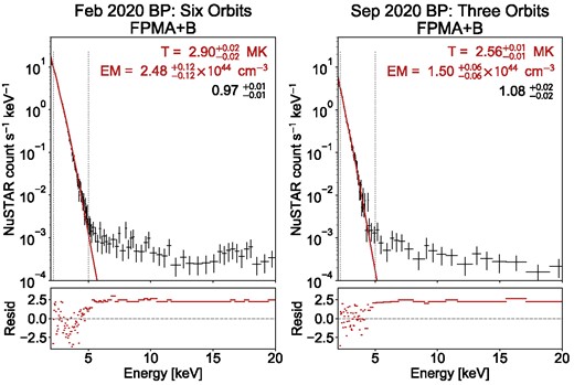
NuSTAR spectra integrated over several hours for the 2020 February and September bright points (left and right panels, respectively), fitted with isothermal models. The 2020 February bright point spectrum is integrated over six orbits (totalling 15.5 ks of data), and the 2020 September bright point spectrum is integrated over three orbits (totalling 8.3 ks of data).
At energies > 5 keV, the integrated bright point spectra are consistent with the aperture component (which is mainly from the cosmic X-ray background) of NuSTAR’s instrumental background (Wik et al. 2014, fig. 9). Though we only plot the spectra up to 20 keV in Fig. A1, we also observe the instrumental lines which dominate the instrumental background between ∼20 and 30 keV.
In these integrated spectra, NuSTAR’s aperture background dominates at energies > 5 keV, and there is no clear additional hot or non-thermal component. Upper limits could be found on the emission that could be present above the instrumental background at these energies, allowing the hot and non-thermal emission from these bright points to be constrained. However, this analysis is beyond the scope of this paper.
