


ABSTRACT
We reported the observations of nulling, subpulse drifting, and moding of radio radiation in pulsar (PSR) B1918+19 at 1250 MHz with the Five-hundred-meter Aperture Spherical radio Telescope. The nulling fraction is 2.6 ± 0.1 per cent and no periodicity of nulling can be seen. We confirmed the existence of three different drift modes (A, B, C) and a disordered mode (N) at 1250 MHz. Unlike the other three modes where the second component of the average pulse profile dominates, the first component of the average pulse profile in mode C is brighter than the other components, the second component shifts forward and the fourth component shifts backward. The bidrifting phenomenon is observed in PSR B1918+19, the drifting of the first and second components is positive, and the drift direction of the fourth component is negative. The drifting rate of the drift bands composed of the first and second components has an obvious evolutionary trend. Mode B has a short duration and no clear trend can be seen. But for mode A, the drift rate of each drift band starts relatively fast, then slows down to a steady state, and finally increases slowly until it enters either null or mode N. Further analysis shows that the emergence and significant variation in the drifting period of multidrifting subpulse emission modes for PSR B1918+19 may be due to the aliasing effect. The interesting subpulse emission phenomenon of PSR B1918+19 at different frequencies provides a unique opportunity to understand the switching mechanism of the multidrift mode of the pulsars.
1 INTRODUCTION
Pulsars (PSRs) are well-known for their highly periodic pulse emissions, characterized by stable average pulse profiles (Helfand, Manchester & Taylor 1975; Kramer 1994; Kramer et al. 1994; Qiao et al. 2001; Shang et al. 2017, 2020, 2021). However, many observations show that the single pulse of most pulsars varies randomly with time in its shape and phase. Only a few pulsars have observed regular changes in single pulses (Backer 1970a; Hesse & Wielebinski 1974; Ritchings 1976; Biggs 1992; Vivekanand 1995; Wang, Manchester & Johnston 2007; Basu et al. 2016). These regular variations, such as pulse nulling, amplitude modulation, and subpulse drifting, provide valuable clues to studying the radiation physics of pulsars.
Pulse nulling is an extreme mode change in which radio emission from a pulsar abruptly ceases. It was first discovered in four pulsars in 1970 (Backer 1970a), and has been observed in nearly 200 pulsars so far. The nulling fraction (NF) measures the percentage of pulses with no detectable emission, indicating the degree of nulling in a pulsar. While NF indicates the presence of nulls, it does not describe their duration or spacing. Previously, pulse nulling has been understudied due to radio telescope sensitivity limitations (Backer 1970a; Ritchings 1976; Janssen & van Leeuwen 2004; Kloumann & Rankin 2010). It has been traditionally believed that pulse nulling is a random phenomenon (Ritchings 1976; Biggs 1992). However, recent studies reveal periodic nulling behaviour in certain classical nulling pulsars, including a periodic switch between nulling and burst states (Herfindal & Rankin 2007; Rankin & Wright 2007; Basu & Mitra 2018; Basu et al. 2019a; Basu, Lewandowski & Kijak 2020b; Zhi et al. 2023b). The in-depth and detailed study of pulse nulling phenomena requires highly sensitive radio telescopes. The subpulse drifting is another intriguing single-pulse phenomenon, which is regarded as a valuable tool for probing the inner magnetospheric structure and radiation mechanism of pulsars (Ruderman & Sutherland 1975; Gil, Melikidze & Geppert 2003; Qiao et al. 2004; Gil, Melikidze & Zhang 2006). Typically, the single pulse of a pulsar consists of one or more subpulses, with its phase and amplitude changing randomly within a periodic radiation window. However, in a small subset of pulsars, there is a phenomenon known as subpulse drifting wherein the phase or amplitude, or both the phase and amplitude of subpulse changes regularly. This phenomenon was first discovered by Drake & Craft (1968). Since then, more than 100 pulsars have been found to exhibit subpulse drifting behaviour (Weltevrede, Edwards & Stappers 2006; Weltevrede, Stappers & Edwards 2007; Basu et al. 2016). Song et al. (2023) reported a large study of periodic behaviour in pulsars based on MeerKAT observations. Mode changes usually refer to the behaviours, i.e. at different time intervals, the continuous single pulse segments show different drifting patterns, or its subpulse shows different radiation intensities or the integrated pulse profile displays different shapes. Interestingly, the mode changes and pulse nulling often coincide with the occurrence of subpulse drifting.
The classic inner gap spark model, also known as the carousel model, suggests that subpulse drifting originated from localized discharges within the inner gap region above the polar cap of pulsar (Ruderman & Sutherland 1975). This model has provided a successful insight into the generation mechanism of subpulse drifting, i.e. the subpulse drifting is generated from the rotating sparks around the magnetic axis. However, the model faces challenges in explaining the complex phenomena associated with changing drifting rates, directions, and switching drifting states (Rankin, Wright & Brown 2013; Rankin & Rosen 2014; Lu et al. 2019; Zhang et al. 2019; Wang et al. 2021). To explore the detailed physical origins of various unique subpulse drifting phenomena, and to further understand and develop the radiation theoretical frameworks of the pulsar, some modified models based on the carousel model have been proposed to explain various unique subpulse drifting phenomena (van Horn 1980; Gil & Sendyk 2000; Qiao et al. 2004; Gogoberidze et al. 2005; Szary & van Leeuwen 2017).
PSR J1921+1948 (B1918+19) was discovered using the Mark 1A radio telescope at Jodrell Bank in 1973 (Davies, Lyne & Seiradakis 1973). Long-term timing observations show that the spin period and periodic derivative of this pulsar are |$0.821\, \rm {s}$| and |$\sim 8.955\times 10^{-16}\, \rm {s\, s^{ -1}}$| (Hobbs et al. 2004), respectively. The characteristic surface magnetic field derived from the spin period and its derivative and the distances derived from the dispersion measures with the electron-density model YMW16 (Yao, Manchester & Wang 2017) are |$\sim 8.68\times 10^{11}\, \rm {G}$| and 4.322 kpc, respectively. The single pulse of this pulsar has been observed and studied at 430 and 327 MHz by Hankins & Wolszczan (1987) and Rankin et al. (2013). Their study results show that the radio radiation of this pulsar exhibits obvious multiple drifting modes. However, the high-frequent observations of the single pulse of this pulsar have not been carefully studied. Recently, we used the Five-hundred-meter Aperture Spherical radio Telescope (FAST) to carry out a high-sensitivity single pulse observation at central frequencies 1250 MHz for this pulsar, which will bring us a valuable opportunity for in-depth and detailed study of the single pulses as well as its physical origin of this pulsar. To study the nulling, subpulse drifting, and moding in PSR J1921+1948 with the single pulse observation of the FAST, the structure of this paper is organized as follows. In Section 2, the observations and data reduction will be presented. In Section 3, the study results of this paper, including the pulse nulling, subpulse drifting as well as the variation of drifting rate, and the number of sparks derived from the subpulse drifting will be presented. The conclusions and discussions will be given in Section 4.
2 OBSERVATIONS AND DATA PROCESSING
The FAST is a Chinese mega-science project located in Pingtang County of Guizhou Province, China. It is the largest single-dish radio telescope in the word, with a total aperture of 500 m and 300 m effective aperture. One of the scientific goals of the FAST is to discover more pulsars and observe them, to establish a pulsar timing array, and participate in pulsar navigation and gravitational wave detection.1 The longitude and latitude of the FAST are 106.9°E and 25.7°N, respectively. The main structure of FAST was completed on 2016 September 25 and it entered the commissioning phase (Jiang et al. 2019, 2020). During the initial commissioning phase from 2016 September to 2018 May, the FAST used an ultra-wideband receiver with a bandpass of 270–1620 MHz (Lu et al. 2019). However, after 2018 May, the FAST switched to a 19-beam receiver with a bandpass of 1.0–1.5 GHz for its observations.
In this paper, the searching mode data of PSR J1921+1948 of the FAST observation project with ID number A3021 will be used for the investigation of nulling and subpulse drifting and moding properties of this pulsar. The observation of this pulsar was carried out with the central beam of the FAST 19-beam receiver. The duration of the observation is 1800 s. The bandpass used in this observation from 1000 to 1500 MHz, the 500 MHz bandwidth is divided into 4096 channels. The time resolution in the observation is 49.152 |$\, \rm {\mu }s$|. Due to unknown and inevitable radio interference at the edge of the bandpass, the frequency range from 1050 to 1450 MHz is used in actual data analysis. All observation data were recorded in PSRFITS format (Hotan, van Straten & Manchester 2004), which is a radio pulsar data storage format based on the Flexible Image Transport System. The observation information of the pulsar is shown in Table 1.
Radio observations of PSR B1918+19.
| Source | Sampling time | Frequency | Bandwidth | Observation data | Observation duration | Single pulse number |
|---|---|---|---|---|---|---|
| (μs) | (MHz) | (MHz) | (s) | |||
| B1918+19 | 49.152 | 1250 | 400 | 2018-Sep-04 | 1800 | 2178 |
| Source | Sampling time | Frequency | Bandwidth | Observation data | Observation duration | Single pulse number |
|---|---|---|---|---|---|---|
| (μs) | (MHz) | (MHz) | (s) | |||
| B1918+19 | 49.152 | 1250 | 400 | 2018-Sep-04 | 1800 | 2178 |
Using the ephemeris of this pulsar provided by the Australia Telescope National Facility Pulsar Catalogue (ANTF pulsar catalogue) 1.70-version2 (Manchester et al. 2005), the search-mode PSRFITS data were folded to obtain the single pulse sequence of PSR B1918+19 with the dspsr package (Hotan et al. 2004; van Straten & Bailes 2011).In observation, radio signals from pulsars are usually more or less contaminated by narrowband non-pulsar signal at a certain frequency. These narrowband non-pulsar radio-frequency interference (RFI) were automatically and manually flagged and removed by using the PAZI and PAZ commands provided by the software package psrchive (Hotan et al. 2004; van Straten, Demorest & Oslowski 2012). For the folding single pulse, we use the psrsalsa (A Suite of ALgorithms for Statistical Analysis of pulsar data) package3 (Weltevrede 2016) to analyse the properties of subpulse drifting, pulse nulling, and moding.
3 RESULTS
The subpulse drifting of PSR B1918+19 is very interesting. As Fig. 1 shows, in the pulse radiation, several nulling pulses are interspersed in the consecutive pulse sequence so that the pulse sequence is split into multiple modules. There are obvious differences in the drift between different modules. In the subsequent analysis, we elaborate on different subpulse behaviours, including the nulling, classification of drift mode, and the evolution of drift rate.
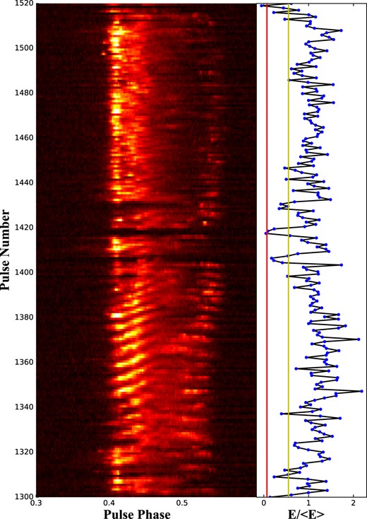
The left panel shows the pulse stack of 220 successive single pulses of PSR B1918+19 obtained from the FAST observation, the centre frequency is 1250 MHz. The right panel shows pulse energy sequences, where the energy has been normalized by the average energy. From left to right, the first vertical line (red) and second vertical line (yellow) in the right panel indicate the thresholds of 3σ and 0.55, respectively.
3.1 Nulling
PSR B1918+19 is a nulling pulsar. Rankin et al. (2013) used Arecibo telescope to study the nuling of PSR B1918+19 at 327 MHz, and obtained NF is |$8.9~{{\ \rm per\ cent}}$|. In Fig. 1, the single pulse plot of 220 consecutive pulses was intercepted. It is clear that there are several nulling pulses are interspersed in the consecutive pulse sequence. To study the nulling phenomenon, the energy distributions of every single pulse in the on-pulse (red histogram) and off-pulse (black histogram) windows are presented in Fig. 2, respectively. The on-pulse window is manually defined as the phase regions from 0.3 to 0.6, the phase range from 0.0 to 0.3 is defined as the off-pulse window. As shown in Fig. 2, the energy distribution of the off-pulse window at 1250 MHz is obvious Gaussian distribution peaking at zero, while the energy distribution of on-pulse windows is a bimodal distribution with two peaks located at zero and ∼1.1, respectively, which means that pulse emission of PSR B1918+19 exhibits nulling phenomenon.
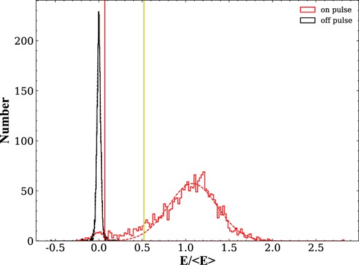
Pulse energy distributions at 1250 MHz. The red and black histograms with the maximum peaks at around 0 and 1.1 represent the energy distributions of on-pulse and off-pulse regions, respectively. From left to right, the first vertical line (red) and second vertical line (yellow) are the 3σ and 0.55, respectively.
The energy of every single pulse in the on-pulse window was calculated, and the nulling pulses were identified from the entire single sequence with the method presented by Ritchings (1976) and Bhattacharyya, Gupta & Gil (2010). In our work, the single pulses with energy lower than 3σ (the red line in Figs 1 and 2, σ is the standard deviation of the Gaussian fit of the off-pulse energy distribution) are classified as the null state, greater than 3σ and less than 0.55E/ < E > (this cutoff is the best one obtained by constant testing, the yellow line in Figs 1 and 2) are classified as the weak state and the single pulses with an energy higher than 0.55E/ < E > are classified as the burst state. Each null pulse is checked individually to avoid identifying weak radiation as a null pulse. In addition, the NF of the on-pulse region was estimated, and it is found that based on the current observation data, 57 null pulses out of 2178 single pulses were found, the NF of PSR B1918+19 at 1250 MHz is |$2.6 \pm 0.1~{{\ \rm per\ cent}}$|. There are 166 weak pulses detected, about 7.6 per cent of the total pulses, which occur at the boundary between the modes. Histograms of the null, weak, and burst lengths in Fig. 3 were calculated to investigate their statistical properties. The results show that the duration of null states ranges from 1 to 9 spin periods, weak states span 1 to 4 spin periods, and burst states extend from 1 to 107 spin periods. Its most distinctive feature is the peak of 23 isolated null pulses, accounting for more than one-third of the total null pulses. Additionally, there are 105 isolated weak pulses, accounting for nearly two-thirds of the total number of weak pulses. In Fig. 4, to investigate the nulling periodicity further, we studied by fourier transform of the null-burst sequence and found that the pulse nulling behaviour of this pulsar has no strict periodicity. However, the weak-burst sequence was Fourier transformed and a clear low-frequency structure was found.
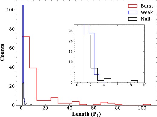
The distribution of the durations of the null, weak, and the burst states for PSR B1918+19.
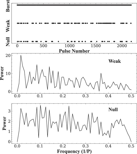
Top: Single pulse with an energy below the 3σ is tagged as null state, greater than 3σ and less than 0.55 is tagged as weak state, and conversely as burst state. Middle: The corresponding power spectrum of the weak states above. Bottom: The corresponding power spectrum of the null states above.
3.2 Subpulse drifting
Hankins & Wolszczan (1987) and Rankin et al. (2013) categorized the drifting behaviour into four different classes: A, B, C, and N. In this work, the broad classification into modes A, B, C, and N follows Hankins & Wolszczan (1987) and Rankin et al. (2013). Fig. 1 shows the essential features of B1918+19’s single pulse behaviour at 1250 MHz. It can be seen that its single pulse clearly shows a subpulse drifting behaviour. Previous studies have been placed in the relatively uncommon conal quadruple category (Rankin 1983, 1993a, b). To investigate the pulse modulation behaviour, we used the psrsalsa package to carry out an analysis of the longitude-resolved fluctuation spectrum (LRFS; Backer 1970b) and two-dimensional fluctuation spectrum (2DFS; Edwards & Stappers 2002) for PSR B1918+19 as shown in Fig. 5. From Fig. 5, we can see that the first and fourth components have a higher modulation index. In the LRFS spectra, there are four features visible, i.e. a prominent low-frequency feature, two clear and one weak feature. Using the same naming convention of (Hankins & Wolszczan 1987; Rankin et al. 2013), three modes with distinct drifting behaviour are called modes A, B, and C, respectively, while the mode with disordered subpulse behaviour is called as mode N. We can see that the periodicities corresponding to the A and B modes are found not only in the first and second components of the integrated profile, but also in the fourth component pair. Significantly, the periodicities corresponding to mode C is only found in the first component. In Figs 6 and 7, displaying examples of the 2DFS and the single-pulse stack of three subpulse drifting modes A, B, and C are presented, respectively. The periodicities corresponding to the A, B, and C modes, which represent the vertical spacing of the driftbands and are conventionally denoted as P3, are very evident. The periods P3 of modes A, B, and C are 6.4P1, 4.0P1, and 2.46P1, respectively. The mode sequence of PSR B1918+19 is listed in Table 2. In addition, one lower frequency periodicity is present, a well-defined one corresponding to a P3 value of some 83P1, which appears to be weak emission related.
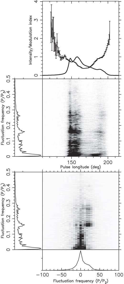
The results of a fluctuation analysis of PSR B1918+19 using psrsalsa. The top panel shows the integrated pulse profile (solid line), the longitude-resolved modulation index (solid line with error bars). The below panel, the LRFS is shown on its horizontal axis the pulse longitude in degrees, which is also the scale for the abscissa of the plot above. Below the LRFS, the 2DFS is plotted. Both the LRFS and 2DFS are horizontally integrated to produce the side-panels of the spectra.
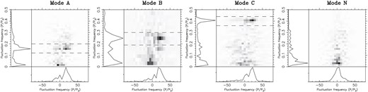
The 2DFS of modes A, B, C, and N. From left to right panels are the 2DFS plots of modes A, B, C, and N, respectively. The peak values for these three drift modes are P3,A ∼ 6.4 P1, P3,B ∼ 4.0 P1, and P3,C ∼ 2.46 P1, respectively.
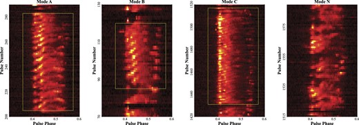
From left to right panels are examples of pulse stacks of modes A, B, C, and N for PSR B1918+19, respectively. Here, the x- and y-axes show the pulse phase and number, respectively.
The mode sequence of PSR B1918+19.
| Pulse range | Mode | Mode length | P3 |
|---|---|---|---|
| (P1) | (P1) | (P1) | |
| 40–62 | B | 23 | 4.0 ± 0.2 |
| 85–120 | B | 36 | 4.0 ± 0.1 |
| 157–180 | B | 24 | 4.0 ± 0.1 |
| 205–283 | A | 79 | 6.45 ± 0.06 |
| 289–355 | A | 67 | 6.41 ± 0.07 |
| 395–450 | A | 56 | 6.41 ± 0.07 |
| 455–540 | A | 86 | 6.33 ± 0.06 |
| 558–655 | A | 98 | 6.25 ± 0.07 |
| 674–780 | A | 107 | 6.37 ± 0.03 |
| 822–892 | A | 71 | 6.13 ± 0.07 |
| 923–944 | B | 22 | 4.0 ± 0.2 |
| 993–1028 | B | 36 | 3.57 ± 0.08 |
| 1043–1090 | A | 48 | 6.33 ± 0.09 |
| 1114–1170 | A | 57 | 5.88 ± 0.24 |
| 1201–1240 | B | 40 | 3.7 ± 0.1 |
| 1315–1404 | A | 90 | 6.37 ± 0.05 |
| 1431–1517 | C | 87 | 2.46 ± 0.03 |
| 1759–1844 | A | 86 | 6.33 ± 0.04 |
| 1863–1966 | A | 104 | 6.41 ± 0.02 |
| 1984–1996 | B | 13 | 3.85 ± 0.15 |
| 2008–2076 | A | 69 | 6.37 ± 0.07 |
| 2096–2166 | A | 71 | 6.33 ± 0.06 |
In Fig. 8, the relative intensities of averaged pulse profiles of the four modes are presented. It is obvious, the averaged pulse profiles specifically extracted for the four modes consist essentially of four emission components, with the third component being weak and less easily resolved. It is interesting to note that the peak of the second component of mode C is shifted towards the leading side while the fourth component seems to be shifted towards the trailing side. As can be seen from Fig. 8, the relative intensity of the average pulse profile in mode N is weaker than that in mode A and B. As in Table 3, we measured the pulse width at 50 per cent (W50) and 10 per cent (W10) of the peak flux for the four modes, which corresponding to separation between 50 per cent peak intensity level of the first and last components and the 10 per cent peak intensity levels of the two components (Basu et al. 2020b). The W50 for the four modes are 49.98°, 51.63°, 53.67°, and 50.62°, respectively. While the W10 of the three modes are 62.28°, 64.36°, 62.88°, and 61.86°, respectively.
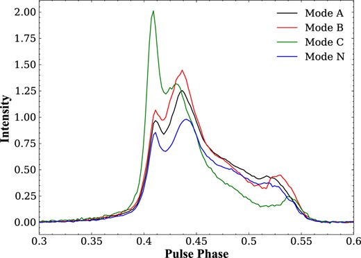
The extracted pulse profiles from modes A, B, C, and N of PSR B1918+19. It is obvious that the pulse profiles of the four modes are distinguishable. The black, red, green, and blue lines are the pulse profiles of modes A, B, C, and N, respectively.
The parameters of the drifting period P2 and drifting rate and amplitude modulation P3 of subpulses for the four radiation modes of PSR B1918+19. W10 and W50 are the pulse widths at 10 per cent and 50 per cent of the peaks of pulse profiles.
| Mode | P3 | P2 | Δϕ | W10 | W50 |
|---|---|---|---|---|---|
| (P1) | (°) | (°/P1) | (°) | (°) | |
| A | 6.4 ± 0.8 | 16.9 ± 0.6 | 2.64 ± 0.34 | 62.28 ± 0.1 | 49.98 ± 0.08 |
| B | 4.0 ± 0.2 | 17.0 ± 1.0 | 4.25 ± 0.33 | 64.36 ± 0.11 | 51.63 ± 0.09 |
| C | 2.46 ± 0.03 | 23.1 ± 1.2 | 9.4 ± 0.5 | 62.88 ± 0.11 | 53.67 ± 0.09 |
| N | 61.86 ± 0.1 | 50.62 ± 0.08 |
In our observations, the most common mode was A (1089 pulses, accounting for 50.0 per cent), followed by N (814 pulses, accounting for 37.4 per cent), B (194 pulses, accounting for 8.9 per cent), and C (81 pulses, accounting for 3.7 per cent). However, these statistics mask considerable variation in the typical sequence length of the patterns: while the C-mode pulses occurred only once, with a length of 81 pulses, the 14 A-mode pulse sequences averaged 78 pulses, the 23 N-mode pulse sequences averaged 35 pulses, the 7 B-mode pulse sequences averaged 27.7 pulses. These modes occur in an order of increasing drift rates, and it exhibits a variety of characteristic mode sequence patterns: null|$\longrightarrow$|N|$\longrightarrow$|A|$\longrightarrow$|B|$\longrightarrow$|N|$\longrightarrow$|null, null|$\longrightarrow$|A|$\longrightarrow$|null, null|$\longrightarrow$|N|$\longrightarrow$|B|$\longrightarrow$|N|$\longrightarrow$|null and null|$\longrightarrow$|N|$\longrightarrow$|C|$\longrightarrow$|null.
3.3 Bidrifting
Thanks to the high signal-to-noise ratio observation data of the FAST, we clearly observed the bidrifting phenomenon of subpulse in PSR B1918+19. For most pulsars with subpulse drifting phenomenon, the direction of subpulse drifting is the same for each subpulse. However, to date, only four interesting pulsars, including PSR J0815+0939, have been found to have significant bidrifting, and the other three are PSRs J1034−3224, J1842−0359, and B2003−08 (Basu et al. 2019a; Basu, Paul & Mitra 2019b; Szary et al. 2020). These bidrifting phenomena of pulsars pose a challenge to the traditional carousel model. It can be understood with some modified models (Szary & van Leeuwen 2017; Wright & Weltevrede 2017). In addition, the origin of the bidrifting behaviour has also been explained using the partially screened gap model by Basu, Mitra & Melikidze (2020a, 2023b) and Basu, Melikidze & Mitra (2022). The main feature of the bidrifting phenomenon is that the drift direction is different in different subpulse components. From Fig. 9, we can see that PSR B1918+19 has bidrifting phenomenon, marked by blue and white dotted lines, respectively. The different drifting directions are separately contributed by different components. The dirfting directions in the pulse windows of the first and fourth components are positive and a negative, respectively. According to Basu et al. (2016), we calculated the phase variation across the pulse window at the peak amplitude and the results are displayed in Fig. 10. The first and second components of pulsar B1918+19 belong to the positive drifting, the corresponding phase variation shows a negative slope as it changes across the pulse window (red shadow in Fig. 10). The fourth component belongs to the negative drifting where the corresponding phase variation shows a positive slope as it changes across the pulse window (blue shadow in Fig. 10). The measured drift rates are 2.64 deg per spin period for mode A, 4.25 deg for mode B, and 9.4 deg for mode C, respectively. The negative drift of the fourth component is weak and not always present.
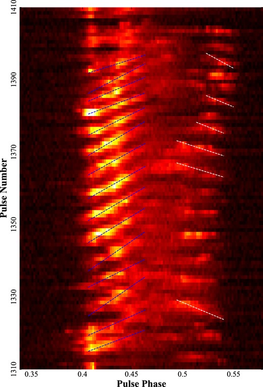
An example of single pulse stacks with overlaid fits to the drift band structure. The blue dashed lines (positive slope) and white dashed lines (negative slope) are a weighted least-squares fit of a straight line to the centroid points for a given drift band.
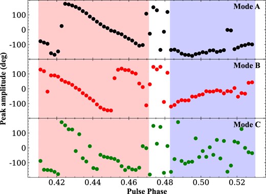
The phase variation across the pulse window at the peak amplitude of three modes. The data points in the top, middle, and bottom panels show the phase variation of modes A, B, and C, respectively.
3.4 Drift rate evolution
The drift rate behaviour of PSR B1918+19 is further discussed by studying the change of the drift rate with the drift band. To calculate the evolution of the drift rate, we follow the method described by Zhang et al. (2019). We first perform a Gaussian function fitting for each subpulse, and set the centroid of Gaussian profiles as the position of each subpulse. We then perform a weighted least-squares fit (blue dashed line in Fig. 9) to the centroid phase of the Gaussian function for each given drift band, and to obtain the drift rate or band slope Δϕ = P2/P3 as well as its uncertainty. In Fig. 9, we intercept a segment of the single-pulse stack of PSR B1918+19 and show the variation of the subpulse drifting rate with time. Fig. 11 shows all drift sequences and the evolution trend of drift rates. Looking at Fig. 11 carefully, although the drift rates in different drift bands are somewhat different, the overall trend appears to be similar for same mode. Mode B has a short duration and no clear trend can be seen. But for mode A, the drift rate of each drift band starts relatively fast, then slows down to a steady state, and finally increases slowly until it enters either null or mode N.
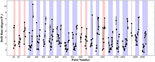
The drift rates variation with the drift bands of PSR B1918+19. Blue and red shadows represent modes A and B, respectively.
3.5 Determination of the number of sparks
Subpulse drifting behaviour was first discovered by Drake & Craft (1968), and generally is described by three parameters, the vertical band spacing at the phase of the same pulse (P3), the horizontal time interval between successive drift bands (P2), and the drift rate (Δϕ = P2/P3). Ruderman & Sutherland (1975) presented an early theoretical model to explanate this phenomenon, i.e. localized pockets of quasi-stable electrical activity called sparks exist near the pulsar’s surface. These sparks move relative to the polar cap surface about the magnetic axis due to the E × B drift, it is like a rotating carousel, which is known as the carousel model. The observed sub-beams of the radiation beam come from these sparks. The subpulses are detected when the line-of-sight sweeps through these sub-beams, and the subpulse drifting phenomenon is produced from the sparks rotating around the rotation axis of the pulsar. If assume that surface sparks are equally spaced in the magnetic azimuth. An aliasing subpulse drifting behaviour will be caused due to the undersampling in the estimation of the true rotation speed of the carousel. The behaviour of the drifting band is usually determined by the carousel rotation rate, P4, and the number of sparks in the carousel, n. If the aliasing exists, the observed P3 follows a specific relation (McSweeney et al. 2019):
where |$\overline{P}_3$| is P3/P1, |$\overline{P}_4$| is P4/P1, and k = [n/|$\overline{P}_4$|] is the aliasing order, in which the square brackets denote rounding to the nearest integer. If the carousel rotation does not change between modes, P4 can be eliminated to yield Δn, where |$\Delta n = n_1-n_2 = n_1 (\overline{P}_{3,2}-\overline{P}_{3,1})/(\overline{P}_{3,2}(1-k*\overline{P}_{3,1}))$| is the difference between the number of sparks of two adjacent modes (McSweeney et al. 2019), where |$\overline{P}_{3,1} \gt $||$\overline{P}_{3,2}$| are the P3 values of two adjacent modes, respectively. Certainly, without aliasing, P3 obeys the other equation, which is P3 = P4/n.
Since the rotation speed of the carousel is determined by the magnetic and electric fields near the pulsar surface, their size and/or orientation cannot be easily changed. In our observations, PSR B1918+19 exhibits multiple drift modes, which may be caused by changes in n or P4. Rankin et al. (2013) believed that P4 remained the same, and the different drift modes were caused by changes in the number of sparks. As the results show in Table 4, we successfully predicted all observed modes, where ni and |$\overline{P}_{3,\mathrm{ i}}$| are the number of sparks and P3 values, respectively, in the assumed mode. Here, we consider the first-order aliasing effect (i.e. k = ±1) and investigate all three observed drift modes using the method proposed by McSweeney et al. (2019). However, due to P3 are harmonically dependent in the spark model (Wright & Fowler 1981), if a hypothetical mode i with |$\overline{P}_{3,\mathrm{ i}}$| to 3.0 P1 is inserted between modes B and C, the harmonic relationship can be restored. The results show that the spark number and P3 values of the three models are obtained successfully, and their P3 values are basically consistent with the observed values.
The deduced carousel parameters for PSR B1918+19.
| nA | nB | (ni) | nC | |$\overline{P}_{3,\mathrm{ A}}$| | |$\overline{P}_{3,\mathrm{ B}}$| | (|$\overline{P}_{3,\mathrm{ i}}$|) | |$\overline{P}_{3,\mathrm{ C}}$| | k | |$\sim \overline{P}_{4}$| | Δn |
|---|---|---|---|---|---|---|---|---|---|---|
| 10 | 9 | (8) | 7 | 6.4 | 4.2 | (3.1) | 2.44 | 1 | 11.9 | 1.04 |
| 9 | 8 | (7) | 6 | 6.4 | 4.0 | (2.9) | 2.28 | 1 | 10.7 | 0.93 |
| 13 | 14 | (15) | 16 | 6.4 | 4.2 | (3.0) | 2.36 | −1 | −11.2 | −0.99 |
| 14 | 15 | (16) | 17 | 6.4 | 4.2 | (3.1) | 2.48 | −1 | −12.1 | −1.06 |
4 CONCLUSIONS AND DISCUSSIONS
In this paper, we studied the nulling and drifting subpulse of PSR B1918+19 with the FAST observation at a centre frequency of 1250 MHz. The nulling fraction at 1250 MHz is 2.6 ± 0.1 per cent. We confirmed the existence of three different drifting modes (A, B, C) and a disordered mode (N) at 1250 MHz. The profile of mode C at 1250 MHz is significantly different compared to the results at low frequencies, and its leading component is significantly stronger than the other radiation components. The first analysis for the radiation properties of PSR B1918+19 was performed in 1987 by Hankins & Wolszczan (1987), who were attracted by the fully conical triple structure of PSR B1918+19, which provided an additional opportunity to study the emission relationship between its inner and outer cones. Using the Arecibo observation at 430 MHz, Hankins & Wolszczan (1987) were able to identify the four basic single pulse modes (A, B, C, and N) and noted specific cyclic relationships between these patterns. In 2013, Rankin et al. (2013) used observations from the same telescope at 327 MHz to explore the geometry of this pulsar and to improve and add to the known single pulse modes of emission. In addition, they proposed a possible carousel structure that exists in the polar cap, which can explain the changes in modes with a simple idea. Although previous studies have reported the subpulse drifting behaviour of PSR B918+19, the sensitivity and frequency band limitations of the telescope did not give detailed results at higher frequencies. The highly sensitive observations of the FAST can provide more detail on the single pulse emission of pulsars at higher frequencies, which is crucial for us to discover the pulsar’s multi-emission properties. Our FAST observations show that there is a complex dynamic mechanism behind the pulsar radio emission, which has important implications for understanding astrophysical processes in extreme environments. In this section, the corresponding discussions and conclusions will be given.
PSR B1918+19 exhibits multiple drift rates and evolutionary features throughout the drift sequences and individual drift bands. We used a linear model to understand the drift rate behaviour within a pulse sequence. We found that the bursts of pulsar B1918+19 usually start irregularly and after a few periods enter the drifting behaviour. After a while, the burst loses its ordered structure and goes into the nulling state or tends to nulling radiation. The drift behaviour is separated by weak and null pulses, and shows different drift behaviour. In our observations, mode A occupies the largest proportion and has the longest duration, mode B generally has a shorter duration, and mode C is observed only once. In our data, the most common mode is A (50.0 per cent), followed by N (37.4 per cent), B (8.9 per cent), and C (3.7 per cent). It can be seen from Fig. 11 that mode A is an evolutionary mode, in which the drift starts from a faster drift rate, evolves towards a slower drift rate and gradually becomes stable, and then begins to evolve towards a faster drift rate before ending. Each drift is followed by a weak radiation of null or approaching null, either short or long. This suggests that the zero point itself may be causally related to the previous drift behaviour. These events can also be seen as drift resets, where the pulsar temporarily evolves to a faster drift rate and then returns to a slower drift rate. This reset could also be due to changes in magnetospheric conditions before reaching the ‘tipping point’.
Many studies have explored the potential correlation between nulling and subpulse drifting in nearly 20 pulsars. Such as the investigations for PSRs J0026−1955 (McSweeney et al. 2022; Janagal et al. 2023), B0031−07 (McSweeney et al. 2017), B0820+02 (Zhi et al. 2023a), B0844−35 (Basu, Mitra & Melikidze 2023c), B0943+10 (Backus, Mitra & Rankin 2011), J1110−5637 (Dang et al. 2022), B1237+25 (Srostlik & Rankin 2005), J1701−3726 (Wang et al. 2023), J1727−2739 (Wen et al. 2016; Rejep et al. 2022), J1741−0840 and J1840−0840 (Gajjar et al. 2017), B1758−29 (Basu et al. 2023c), J1926−0652 (Zhang et al. 2019), B1944+17 (Serylak, Stappers & Weltevrede 2009; Kloumann & Rankin 2010b), B2003−08 (Basu, Paul & Mitra 2019b), B2000+40 (Basu et al. 2020b), B2303+30 (Redman, Wright & Rankin 2005), B2319+60 (Rahaman et al. 2021; Chen et al. 2022), B0818−41 (Bhattacharyya et al. 2010), and B0809+74 (van Leeuwen et al. 2003; Basu et al. 2023a). Among them, the investigation of PSR B0818−41 demonstrates a case where a decline in the pulsar drift rate coincides with a gradual decrease in intensity before the start of a null. The observations of PSR B0809+74 also show an association between nulls and subpulse drifting, where the drift rate deviates from the norm following instances of nulls, and postulated, using the partially screened gap model, that a form of ‘reset’ occurs within the radio emission of pulsar engine during nulls, subsequently influencing the conditions of the magnetosphere (van Leeuwen et al. 2003). However, a recent study at 150 MHz of Basu et al. (2023a) seem to suggest that the transition to nulling follows shortly after the pulsar switches to the slow-drift mode, rather than at the boundary between the modes. Wang et al. (2007) proposed that radio emission can abruptly cease or commence when the charge or magnetic configuration in the magnetosphere reaches a critical ‘tipping point’. However, the exact triggering mechanism for such a stimulus remains unknown. There are several suggestions for such changes, like the changes in the global magnetospheric configuration (Timokhin 2010; Melrose & Yuen 2014; Yuen & Melrose 2017) or rapid modifications in the surface magnetic fields (Geppert et al. 2021). Moreover, in the case of PSR J1822−2256, Janagal et al. (2022) also presented a piece of evidence to show a relationship between nulling and mode changing, where a null typically precedes most occurrences of their mode D. These correlations suggest potentially strong links between the emission mechanisms and magnetosphere dynamics, the nulls and subpulse drifting. It is important to highlight that occurrences, where nulls affect the drifting behaviour leading up to them, are relatively uncommon, especially in contrast to the more extensively studied effect of nulls on subsequent burst sequences (e.g. Lyne & Ashworth 1983; van Leeuwen et al. 2003; Janagal et al. 2022). A comprehensive understanding of these infrequent cases could offer valuable insights into the intricate dynamics associated with nulls and subpulse drifting in pulsars.
Rankin et al. (2013) observed at 327 MHz that the mode N is accompanied by a periodicity of P3 = 12P1, produced in part by repeating null bunches embedded in the mode N. Assuming that PSR B1918+19 has a circulation time P4 of about 12 P1, the modes N, A, B, and C reflect the carousel configuration of the 11, 10, 9, and 7 sub-beams, respectively, and there is a mode P3 of about 3.0 P1 between modes B and C. We assume that the multiple drift modes of PSR B1918+19 are caused by first-order aliases, and that we have a new mode between modes B and C, P3 to 3.1 P1. Then, the first-order solutions of all three drift modes are calculated. As can be seen from Table 4, when the representative solution is k = 1, there are [nA, nB, nC] = [10, 9, 7] sparks, and the rotation period is |$\overline{P}_4 = 11.9 P_1$|. At k = −1, there are [nA, nB, nC] = [14, 15, 17] sparks with a rotation period of |$\overline{P}_4 = -12.1 P_1$|. At the same time, the moderate rotation period is |$10 \le |\overline{P}_4| \le 13$|. It should be pointed out that polarization measurements were not included in this paper, and further studies on the polarization characteristics of different drifting modes are very valuable, which may give more accurate results for the magnetospheric structure and detailed physical processes, and provide an important understanding of pulsar radiation physics.
Of course our estimates of the sparking configuration are idealized. Recent studies have shown that the underlying assumptions of the inner vacuum gap (IVG) model have several shortcomings (see e.g. van Leeuwen & Timokhin 2012). For example, the surface magnetic field above the polar cap is dominated by non-dipolar magnetic fields (e.g. Geppert 2017; Arumugasamy & Mitra 2019; Pétri & Mitra 2020) which makes it unlikely to have a circular carousel. Recent works have focused on updates to the carousel model like presence of elliptical carousels (Wright & Weltevrede 2017), magnetospheric interactions (Wright 2022), as well as alternate models based on a partially screened gap (Gil et al. 2003), with sparks lagging behind the rotation motion of the star (Basu et al. 2020b; Basu et al. 2023a).
ACKNOWLEDGEMENTS
This work was supported by the Major Science and Technology Program of Xinjiang Uygur Autonomous Region (Nos. 2022A03013-3 and 2022A03013-4), the Academic New Seedling Fund Project of Guizhou Normal University (No.[2022]B18), and the Scientific Research Project of the Guizhou Provincial Education (Nos. KY[2022]137 and KY[2022]132), the Guizhou Provincial Science and Technology Foundation (No. ZK[2022]304), the National Natural Science Foundation of China (NSFC) project (Nos. 12203092 and 12363005), the Natural Science Foundation of Xinjiang Uygur Autonomous Region (No. 2022D01B71), the National SKA Program of China (No. 2020SKA0120100). At the same time this work made use of the data from the Five-hundred-meter Aperture Spherical radio Telescope (FAST). FAST is a Chinese national mega-science facility, built and operated by the National Astronomical Observatories, Chinese Academy of Sciences.
DATA AVAILABILITY
The data underlying this article will be shared on reasonable request to the corresponding author.
