


ABSTRACT
The ages and metallicities of globular clusters play an important role not just in testing models for their formation and evolution but also in understanding the assembly history of their host galaxies. Here, we use a combination of imaging and spectroscopy to measure the ages and metallicities of globular clusters in M31, the closest massive galaxy to our own. We use the strength of the near-infrared calcium triplet spectral feature to provide a relatively age-insensitive prior on the metallicity when fitting stellar population models to the observed photometry. While the age–extinction degeneracy is an issue for globular clusters projected on to the disc of M31, we find generally old ages for globular clusters in the halo of M31 and in its satellite galaxy NGC 205 in line with previous studies. We measure ages for a number of outer halo globular clusters for the first time, finding that globular clusters associated with halo substructure extend to younger ages and higher metallicities than those associated with the smooth halo. This is in line with the expectation that the smooth halo was accreted earlier than the substructured halo.
1 INTRODUCTION
Globular clusters (GCs) are a powerful tool to study galaxy formation (see reviews by Brodie & Strader 2006; Forbes et al. 2018) as the properties of GCs observed today reflect not only the conditions of their formation but also the physics of GC survival. Found in virtually all galaxies with stellar masses above 109 M⊙ (and most galaxies more massive than 107 M⊙; Harris, Harris & Alessi 2013; Eadie, Harris & Springford 2022), they are significantly brighter than individual stars, allowing them to be studied at much greater distances. The oldest GCs serve as fossils of the earliest stages of galaxy formation, while the continuous formation of GCs until today (e.g. Martocchia et al. 2018; Bastian et al. 2019) allows them to trace the full history of galaxy formation. GC ages not only provide an important test of theories of how GCs formed and evolved but also can provide important constraints on how galaxies form and assemble.
In this paper, we use the term GC for any star cluster older than ∼1 Gyr and young massive cluster (YMC) for any star cluster younger than this age. This division corresponds to the transition for a massive cluster from being dominated by formation physics to disruption physics and in stellar evolution terms to when the red giant branch starts to make a significant contribution to the luminosity of the cluster.
Two broad classes of models for GCs have been proposed. Motivated by the old ages of Milky Way (MW) GCs (e.g. Janes & Demarque 1983; VandenBerg et al. 2013; Valcin et al. 2021) and the lack of easily observable star clusters forming today in the MW massive enough to survive a Hubble time, the first class of models (e.g. Peebles 1984; Trenti, Padoan & Jimenez 2015) invokes special conditions in the early Universe. In these models, GCs form during or even before the epoch of reionization (z ≳ 6, lookback times ≳13 Gyr), often in their own dark matter haloes. In the second class of models (e.g. Elmegreen & Efremov 1997; Elmegreen 2010; Kruijssen 2015), motivated by observations of star clusters of GC mass or greater forming in starburst galaxies today (e.g. Whitmore & Schweizer 1995; Holtzman et al. 1996; Adamo et al. 2020), GC formation is the natural outcome of intense star formation. In the first class of models, all GCs in all galaxies should have formed in the first Gyr of the Universe; in the second, the distribution of GC ages should be broader and should vary with galaxy assembly history. Quantitative models of GC formation (e.g. Li & Gnedin 2014; Pfeffer et al. 2018; Valenzuela et al. 2021; Rodriguez et al. 2023) make predictions for the age distribution of GCs that can be compared to observations.
GCs are also powerful probes of the formation and assembly history of galaxies. Since a large star formation rate density is required to form a massive, compact star cluster, the ages of GCs trace periods of intense star formation. If the age and metallicity of a GC are known, the galaxy mass–metallicity relation (see review by Maiolino & Mannucci 2019) can be inverted to give the likely mass of the galaxy the GC formed in (Kruijssen et al. 2019). With multiple GCs, the mass assembly history of a galaxy can be constrained. The presence of GCs with a significant range of metallicities at the same age implies that those GCs formed in different mass galaxies. The presence of at least two branches of the MW GC age–metallicity relationship was used to argue that the older branch was the in situ population and the younger branch was the accreted population (Forbes & Bridges 2010; Leaman, VandenBerg & Mendel 2013). This association was confirmed by the younger branch GCs having the same orbits as accreted satellite galaxies (e.g. Massari, Koppelman & Helmi 2019). By folding in constraints on the orbits of GCs, the merger tree of a galaxy can be reconstructed in detail as was done for the MW by Kruijssen et al. (2020) since earlier mergers and more massive mergers should deliver their GCs to smaller galactocentric radii (Pfeffer et al. 2020).
Beyond the Local Group, GCs cannot be resolved into their constituent stars and have to be studied using their integrated light. Despite their importance, measuring reliable GC ages from their integrated light remains a challenge. Optical photometry suffers from strong age–metallicity and age–extinction degeneracies (e.g. Worthey 1994; Anders et al. 2004; de Meulenaer et al. 2014) in that old ages and higher metallicities both make a stellar population redder as can the effects of interstellar extinction. While ultraviolet or near infrared (NIR) photometry can be used to break this degeneracy, obtaining deep enough photometry for a significant sample of GCs can be observationally expensive. Spectroscopy can also provide ages but the quality of spectra required is likewise observationally expensive for significant samples. While spectroscopy does not suffer from the age–extinction degeneracy, it can suffer from a degeneracy between the morphology of the horizontal branch and age (see Cabrera-Ziri & Conroy 2022 for a detailed discussion).
Usher et al. (2019b) used optical photometry and spectroscopy of the near-infrared calcium triplet (CaT) to derive ages and metallicities for GCs in three massive early-type galaxies from the SAGES Legacy Unifying Globulars and GalaxieS (SLUGGS) survey (Brodie et al. 2014) and the MW. Usher et al. (2019a) showed that the strength of the CaT is a reliable and age-independent measure of metallicity for stellar populations older than a couple of Gyr. Usher et al. (2019b) used these metallicities as priors when fitting the photometry with stellar population models to measure ages. In line with previous work (e.g. Usher et al. 2015; Powalka et al. 2016) that found that the GC colour–metallicity or colour–colour relationship varies between galaxies, Usher et al. (2019b) found that these four galaxies show widely different distributions of GCs in age–metallicity space, suggesting different assembly histories and disfavouring models where the majority of GCs form in the early Universe.
As the nearest (780 kpc; Conn et al. 2012) massive (stellar mass ∼1011 M⊙; Tamm et al. 2012) galaxy to the MW, M31 provides an important test of techniques for studying GCs using their integrated light. M31 is close enough that its GCs can be observed in ways that are impractical for more distant galaxies – its GCs can be resolved into their constituent stars using space-based observations and high signal-to-noise ratio (S/N), high-resolution integrated spectroscopy can be obtained in a reasonable amount of time − yet it is distant enough, that is relatively straightforward to obtain integrated photometry and spectroscopy of its GCs.
There is a long history of studying the metallicities and ages of GCs in M31 using their integrated light (e.g. van den Bergh 1969; Burstein et al. 1984; Beasley et al. 2005; Puzia, Perrett & Bridges 2005; Galleti et al. 2009; Caldwell et al. 2011; Sakari & Wallerstein 2022). The superior spatial resolution of the Hubble Space Telescope (HST) allows the star clusters of M31 to be resolved into their individual stars. In most cases, the resulting colour–magnitude diagrams only reach the upper red giant branch (e.g. Holland, Fahlman & Richer 1997; Rich et al. 2005; Perina et al. 2009) but in the case of B379-G312, the photometry reaches below the main sequence turn-off, allowing the age to be measured directly (Brown et al. 2004; Ma et al. 2010). With shallower photometry, lower limits on the age can be placed and the presence of a blue horizontal branch can be used as evidence for an old stellar population (e.g. Perina et al. 2011). While most M31 GCs seem to be old (≳10 Gyr) and M31 hosts a population of YMCs (≲1 Gyr; e.g. Hodge 1979; Elson & Walterbos 1988; Caldwell et al. 2009; Johnson et al. 2016), the existence of a population of younger GCs (between 1 and 10 Gyr) has been debated (e.g. Burstein et al. 2004; Beasley et al. 2005; Caldwell et al. 2011; Perina et al. 2011).
In this paper, we extend the analysis of Usher et al. (2019b) to M31 by using literature spectra described in Section 2 to measure the metallicity of 290 GCs using the strength of the CaT spectral feature (Section 3). In Section 4, we use these metallicities as a prior when deriving their ages from their optical photometry before summarizing our work in Section 5.
2 LITERATURE DATA
2.1 Spectroscopy
We used spectra of the CaT region from Caldwell et al. (2009) and from Sakari & Wallerstein (2016, 2022) and Sakari et al. (2021). Caldwell et al. (2009) observed over 500 star clusters in M31 using the Hectospec multifibre spectrograph (Fabricant et al. 2005). The Hectospec spectra cover 3700–9200 Å at a resolution of ∼5 Å and a dispersion of 1.2 Å. We restricted ourselves to the subsample of 316 star clusters determined by Caldwell et al. (2011) to be old. These Hectospec spectra all lie within 20 kpc in projection of the centre of M31.
Sakari & Wallerstein (2016) observed 27 GCs at a range of galactocentric distances using the Dual Imaging Spectrograph (DIS) on the 3.5 m telescope at Apache Point Observatory and 5 GCs using the Sparsepak fibre unit (Bershady et al. 2004, 2005) and the Bench Spectrograph (Bershady et al. 2008; Knezek et al. 2010) on the Wisconsin-Indiana-Yale-NOIRLab (WIYN) 3.5 m telescope. Sakari et al. (2021) observed a single GC (G001-MII) with DIS and the Apache Point Observatory 3.5 m telescope and Sakari & Wallerstein (2022) observed 30 GCs in the outer halo of M31 with same instrument and telescope. The DIS spectra cover 8000–9100 Å at resolution of R ∼ 4000, and the WIYN spectra cover 8300–8800 Å at resolution of R ∼ 9000. We do not include the spectrum of B457-G097 from Sakari & Wallerstein (2016) in our analysis since Sakari & Wallerstein (2016) suggest that they observed a different object given the substantial differences in radial velocity (∼300 km s−1) and metallicity (∼0.5 dex) between their measurements and literature values; we do use the spectrum of B457-G097 from Caldwell et al. (2011). Nor do we include the spectrum of dTZZ-05 as suggested by Sakari & Wallerstein (2022) since the measured radial velocity is more similar to an MW star than an M31 GC.
2.2 Imaging
We preferred the Sloan Digital Sky Survey (SDSS; York et al. 2000) ugriz photometry of Peacock et al. (2010) when available. For more recently discovered GCs in the SDSS footprint, we used the SkyServer1 service to download SDSS Data Release 17 (DR17; Abdurro’uf et al. 2022) model photometry for each GC.We applied the 0.04 mag correction to bring the u band on to the AB magnitude system. For halo GCs not covered by SDSS, we used the Pan-Andromeda Archaeological Survey (PAndAS) Canada France Hawaii Telescope MegaCam gi photometry from Huxor et al. (2014).
3 CALCIUM TRIPLET-BASED METALLICITIES
We measure the metallicities of the M31 GCs using the strength of the CaT rather than relying on the Caldwell et al. (2011) Lick index-based metallicities to both maintain commonality with Usher et al. (2019b) and since the strength of the CaT shows little dependence on age (e.g. Vazdekis et al. 2003; Usher et al. 2019a). We measure the strength of the CaT using the technique of Foster et al. (2010) and Usher et al. (2012, 2019a). We use the same python code as in Usher et al. (2019a) to fit the observed spectra with a linear combination of stellar templates (we use the same templates as Foster et al. 2010; Usher et al. 2012, 2019a), normalize the continuum (using the same parameters as in Usher et al. 2019a), and measure the combined CaT strength of all three lines from the fitted templates using the same index definition (that of Armandroff & Zinn 1988) as in our previous work. We refer the interested reader to Usher et al. (2019a) for details of the measurement process and a detailed discussion of potential systematics. To avoid systematics due to poor sky subtraction or low S/N, we only measure spectra with S/N greater than 20 Å−1. For the Sakari et al. spectra, we also excluded a handful of spectra with higher S/N that showed strong sky subtraction residuals.
Unfortunately, the measured strength of the CaT depends on the spectral resolution or velocity dispersion, with the CaT strength being systematically lower at lower spectral resolutions, especially at high metallicity (e.g. Cenarro et al. 2001; Usher et al. 2019a). While the resolution of the Sakari et al. spectra is high enough not to be significantly affected by this effect, the Caldwell et al. (2011) spectra are low enough resolution to be. We used high S/N spectra of the CaT region of 27 GCs from the WiFeS Atlas of Galactic Globular cluster Spectra (WAGGS) survey (Usher et al. 2017, 2019a), which span the range of MW GC metallicities (−2.4 < [Fe/H] < −0.1) to derive an empirical correction for the effects of velocity dispersion on the measured strength of the CaT. We first smoothed each of the WAGGS spectra to a range of velocity dispersions between 10 and 100 km s−1 and measured the strength of the CaT on each smoothed spectra. For each WAGGS GC, we then fit a cubic spline between the measured velocity dispersion and the measured CaT strength. We used these splines to estimate the CaT strength at a velocity dispersion of 72.3 km s−1, the median of the velocity dispersions fitted to the Caldwell et al. (2011) spectra, for each of the WAGGS GCs. We then fit a cubic relationship between the CaT strength measured on the spectra broadened to 72.3 km s−1 and the CaT strength measured on the original, unbroadened spectra. This broadening is consistent with the line spread function of Hectospec (σ = 78 ± 4 km s−1) found by Fabricant et al. (2013) at 8600 Å once the line spread function (σ = 19 km s−1) of the Keck DEIMOS (DEep Imaging Multi-Object Spectrograph) template spectra is accounted for. We used this relationship to correct each of the CaT strengths measured from the Caldwell spectra. To estimate the systematic uncertainty introduced by this correction, we repeated the correction at 62.7 and 86.7 km s−1, the 2.3 and 97.7 percentiles of the velocity dispersion distribution measured from the Caldwell et al. (2011) spectra. We used these, respectively, to correct the upper and lower uncertainties on the measured CaT strength. In terms of metallicity, the strength of the correction varies from 0.09 dex at [Fe/H] = −1 to 0.42 dex at [Fe/H] = 0 as seen in Fig. 1.
![Comparison of the CaT [Fe/H] values measured from the Caldwell et al. (2011) spectra and the [Fe/H] values measured by Caldwell et al. (2011) using Lick Fe indices using the same spectra. The top panel shows the [Fe/H] calculated from the CaT values uncorrected for the effects of spectral resolution; the bottom panel shows the [Fe/H] calculated from the corrected CaT values. The solid line in the upper panel is the spectral resolution correction we apply to the CaT values. The median uncertainties are shown in the lower panel. The dashed line is the one-to-one line and the dotted lines show ±0.1 dex. The metallicities measured using the two different methods agree within 0.25 dex.](https://oup.silverchair-cdn.com/oup/backfile/Content_public/Journal/mnras/528/4/10.1093_mnras_stae282/1/m_stae282fig1.jpeg?Expires=1750232585&Signature=oaiVAFE7F2rOq4S2SwD1nxo0pvBYTVi~Uly2Cd-HWpnVWPx6ACwLIehkGF~wZ419o8jEExW5X4QiZbuISI5k09k6WUjbZeHAqrLX7JOzIb7h-0JSVsqRHmaWdcpuGJvSvJvGDqrBJzHof-tAfoiKoMYYpVD95wbPESZjIB-f~tQKDeZg-E1SBIXRmmpUieX~SPsKDEz4PHKs-x-ZRAEkjwhXBPtcVT5Wz5Hpo6EHwz9eRgK53PC~xrtxI7XCvazZrI5TZbxNDJOTBnFxdTF60MzxjTqmtlefw9sXQau77YnirnTt6FsuB9h1A81PrgLB4BECrDrACf01Pq9x6Cc0GA__&Key-Pair-Id=APKAIE5G5CRDK6RD3PGA)
Comparison of the CaT [Fe/H] values measured from the Caldwell et al. (2011) spectra and the [Fe/H] values measured by Caldwell et al. (2011) using Lick Fe indices using the same spectra. The top panel shows the [Fe/H] calculated from the CaT values uncorrected for the effects of spectral resolution; the bottom panel shows the [Fe/H] calculated from the corrected CaT values. The solid line in the upper panel is the spectral resolution correction we apply to the CaT values. The median uncertainties are shown in the lower panel. The dashed line is the one-to-one line and the dotted lines show ±0.1 dex. The metallicities measured using the two different methods agree within 0.25 dex.
We used the empirical correction of Usher et al. (2019a, their equation 1) to translate our CaT values into metallicities. The Usher et al. (2019a) relation is based on MW and MW satellite GCs. Since CaT is sensitive to the [α/Fe] abundance ratio (Brodie et al. 2012; Sakari & Wallerstein 2016; Usher et al. 2019a), if the [α/Fe]–[Fe/H] relation of M31 GCs is different, our [Fe/H] measurements will be biased. In Fig. 1, we show a comparison of our CaT-based [Fe/H] with the [Fe/H] measured by Caldwell et al. (2011) using Lick Fe indices and an empirical relationship before and after performing the spectral resolution correction. The root mean squared (RMS) difference between the two metallicities is 0.25 dex, which is in agreement with the uncertainties. While the correction for spectral resolution improves the agreement at the highest metallicities, small (<0.2 dex) systematic differences remain, with the CaT metallicities being systematically higher near [Fe/H] ∼ −1.5 and systematically lower at [Fe/H] ∼ −0.5. We note that both the Caldwell et al. (2011) metallicities and our CaT metallicities are based on simple empirical relationships between the strength of spectral indices and the metallicities of MW GCs. Some level of systematic difference is unsurprising, given that the Fe Lick indices used by Caldwell et al. (2011) and the CaT used in this work show difference dependences on [α/Fe] and the simple empirical relations used by Caldwell et al. (2011, bilinear) and Usher et al. (2019a, linear).
In Fig. 2, we show a comparison between the CaT [Fe/H] values measured from the Sakari & Wallerstein (2016) and Caldwell et al. (2011) spectra. The agreement between the two is excellent with an RMS difference of 0.11 dex in agreement with the statistical and expected systematic uncertainties. In Fig. 3, we compare our CaT metallicities with those from Sakari & Wallerstein (2022). Again we see good agreement at most metallicities, although the Sakari & Wallerstein (2022) metallicities are systematically higher at metallicities below [Fe/H] = −2. Our measurement for EXT8 ([Fe/H] = −2.71 ± 0.07) is closer to the value from high-resolution spectroscopy (Larsen et al. 2020, [Fe/H] = −2.91 ± 0.04) than the CaT-based value from Sakari & Wallerstein (2022) ([Fe/H] = −2.27 ± 0.10). In Fig. 4, we compare our metallicities with those based on analysis of high-resolution integrated light. We see good agreement with the optical studies of Colucci, Bernstein & Cohen (2014), Sakari et al. (2015), and Larsen et al. (2022) as well as the near-infrared study of Sakari et al. (2016) using either the Caldwell et al. or Sakari et al. spectra.
![Comparison of the CaT [Fe/H] values measured in this work from the Sakari & Wallerstein (2016) spectra and the Caldwell et al. (2011) spectra. The dashed line is the one-to-one line and the dotted lines show ±0.1 dex. The metallicities measured using the two different sets of spectra agree within 0.1 dex.](https://oup.silverchair-cdn.com/oup/backfile/Content_public/Journal/mnras/528/4/10.1093_mnras_stae282/1/m_stae282fig2.jpeg?Expires=1750232585&Signature=jug~EjXj4PQS2epvT4I5dQxUZPSatI3WaSGTdwQPy2SrMnnmt1U3~LVmOmmV05Agpm1QLatBmFNzPLrPnTL2F5iRfdBvw8dWoS-ujcvCSvPL7lGjtnp5TVByHe4NWE2KFqW5OejMZwoz1jwOAiKMwJ-1Zti5uc0s4em6Y-uNDjyf4Y-iKxJh--lQxex-Iqil80ltXaZIbS8o54ZnZfzog8YBvnSSTnDtiTZIxEdR2qvhMm~C1W5g-exEFQacN4GXExkOfv2-TQGQDpH2r65kjhB-3WBzDuqHijWmbb9tK~lDzZbA5fID8r~C9UMM~QKXpKsSTsaDougA8RB7t4JvEQ__&Key-Pair-Id=APKAIE5G5CRDK6RD3PGA)
Comparison of the CaT [Fe/H] values measured in this work from the Sakari & Wallerstein (2016) spectra and the Caldwell et al. (2011) spectra. The dashed line is the one-to-one line and the dotted lines show ±0.1 dex. The metallicities measured using the two different sets of spectra agree within 0.1 dex.
![Comparison of the [Fe/H] values measured in this work and those measured by Sakari & Wallerstein (2022) both using the strength of the CaT and the spectra from Sakari & Wallerstein (2022). The dashed line is the one-to-one line and the dotted lines show ±0.1 dex. In general, there is good agreement between the two studies except below [Fe/H] = −2 where the Sakari & Wallerstein (2022) metallicities are systematically higher.](https://oup.silverchair-cdn.com/oup/backfile/Content_public/Journal/mnras/528/4/10.1093_mnras_stae282/1/m_stae282fig3.jpeg?Expires=1750232585&Signature=ZwZLyOlPK37rztC-2yy0oe6M52IkOFUDnxSUt7s4V7z-h8-YyH3jETlAxluydtg~7nSwjCBCHB~tQyPouxQH-nbfNmOArYUDaz~aFeBSJytxX-bUHgnLXfT1BeF2rWv4zMZOlHS2se0k-wo5NT3kBtrDa38hILiYvlvwULxf39XZ3JCHo5hh~TqwB266FK3Z7rIRqaQpy6dM-uHQSq5zBPHTQr7WHVsRMCdpkXyjKLtm589xospYPsHmf8YKkJLPg2j2CUILYbt4VVFkkCV9gIYWhnGlr30goy5SEU9hSXN7hin86KwDlCT9RLzRpfhyEsCTedcKsmA~-xmFXP68qg__&Key-Pair-Id=APKAIE5G5CRDK6RD3PGA)
Comparison of the [Fe/H] values measured in this work and those measured by Sakari & Wallerstein (2022) both using the strength of the CaT and the spectra from Sakari & Wallerstein (2022). The dashed line is the one-to-one line and the dotted lines show ±0.1 dex. In general, there is good agreement between the two studies except below [Fe/H] = −2 where the Sakari & Wallerstein (2022) metallicities are systematically higher.
![Comparison of the CaT [Fe/H] values with literature [Fe/H]. The left panel shows a comparison with the Caldwell et al. spectra and the right with the Sakari et al. spectra. The dashed line is the one-to-one line and the dotted lines show ±0.1 dex. There is generally good agreement between our metallicity measurements and those from the literature high-resolution studies.](https://oup.silverchair-cdn.com/oup/backfile/Content_public/Journal/mnras/528/4/10.1093_mnras_stae282/1/m_stae282fig4.jpeg?Expires=1750232585&Signature=z0Lfrv~4Qeq0WqZFbOqPniL9Jh9XNW0FzFRbomqVL9DKwgn622lctOQioja230TSGXHHqWrmZ~IJk3pCB8-pPO-YV1M6UwyDR~dL64ulNcF2KFVZd1~qSpTDPdRX544q5RO8l2NJqGSqjNsUaPyWMo3WyPkPxGG5zbsGFhPBXGcQvZAdMPjwk9UJw-0173de1udEiCiymNJDnD-bSjXA2qoA1BhE-sVb90auFj6anvqoq55GDmZjKSMOSNWZfF5RB62KVm3JE5roRxeC4wAXFl4q5anWM3z6wjPpOQh8BRVISxKbiKcQraqQsQBhqj73EikKFUiyXryotPiZf~8sNA__&Key-Pair-Id=APKAIE5G5CRDK6RD3PGA)
Comparison of the CaT [Fe/H] values with literature [Fe/H]. The left panel shows a comparison with the Caldwell et al. spectra and the right with the Sakari et al. spectra. The dashed line is the one-to-one line and the dotted lines show ±0.1 dex. There is generally good agreement between our metallicity measurements and those from the literature high-resolution studies.
4 AGE MEASUREMENTS
To determine ages, we used the Monte Carlo Markov chain (mcmc) code first presented in Usher et al. (2019b), which we now name mcmame (Monte Carlo Metallicity, Age, Mass, and Extinction). In this analysis, we sample age, metallicity, mass, and reddening posteriors of a grid of stellar population models subject to the constraints provided by the photometry and optionally the CaT metallicity. As in Usher et al. (2019b), we use emcee (Foreman-Mackey et al. 2013) with a parallel-tempered ensemble sampler (Vousden, Farr & Mandel 2016) with 8 temperatures, 64 walkers, 200 burn-in steps, and 2560 production steps. We use the same stellar population models (fsps Conroy, Gunn & White 2009; Conroy & Gunn 2010, calculated with the MIST isochrones Choi et al. 2016 and the MILES spectral library Sánchez-Blázquez et al. 2006), and mass priors (flat in log mass), but use slightly different age priors (flat between 1 Myr and 15 Gyr) and metallicity priors (flat between [Fe/H] = −3.0 and +0.5) than in Usher et al. (2019b).Unlike in Usher et al. (2019b) where the reddening vector from Schlafly & Finkbeiner (2011) was assumed for all ages and metallicities, we used fsps to calculate the age and metallicity-dependent reddening vector using the Cardelli, Clayton & Mathis (1989) MW extinction curve. At low extinction values this assumption is valid, but for larger values it breaks down since the effect of extinction depends on the shape of the spectral energy distribution within a filter passband, with a population with a bluer spectrum being more affected than a redder one. For reddening, we need to adopt different priors than in Usher et al. (2019b) given that M31 has substantial internal extinction, unlike the massive early-type galaxies studied in Usher et al. (2019b).
As a first-order approximation, we can think of most of the internal extinction in M31 coming from a thin disc of gas and dust. The majority of old and intermediate-age GCs should be either in front of or behind this disc as star clusters would not survive long orbiting in the same plane as massive molecular clouds (Elmegreen 2010; Kruijssen 2015). Thus, the prior on the extinction should be bimodal, with one peak corresponding to the foreground extinction and one peak corresponding to the extinction of the foreground plus the disc of M31. In principle, a GC should have equal probability of being in front of or behind the disc. However, in a magnitude-limited sample, GCs on the far side of the disc will be fainter and more likely to fall out of the selection.
The extinction can be modelled through various methods including from far-infrared and sub-millimetre observations (e.g. Schlegel, Finkbeiner & Davis 1998; Whitworth et al. 2019) and by modelling the colours of stars (e.g. Dalcanton et al. 2015). Unfortunately, the distribution of gas and dust is filamentary, with significant changes in the extinction value on comparable scales to the radius of a GC (e.g. Bonatto, Campos & Kepler 2013; Saracino et al. 2019; Bonatto & Chies-Santos 2020). While for M31, extinction can be modelled on the scales of ∼30 pc (e.g. Dalcanton et al. 2015; Whitworth et al. 2019), for more distant galaxies it can only be modelled on larger scales. To mimic the low spatial resolution available for more distant galaxies, we used the Schlegel et al. (1998) extinction maps, which have a resolution of 6.1 arcmin (∼1.4 kpc at the distance of M31). We modelled the contribution of the disc of M31 to the extinction as a Gaussian with a mean provided by the value of the Schlegel map at that location and a standard deviation equal to 50 per cent of the mean. We used the median extinction from the Schlegel map of GCs outside of the disc of M31 (0.08 mag) as the mean value of the foreground contribution and assumed a dispersion of 0.03 mag on the foreground. In our bimodal extinction prior, we assigned equal weight to the foreground and M31 disc components. In all cases, we enforced a further constraint that the extinction must be positive.
An example of the posterior distribution for B379-G312 is plotted in Fig. 5. This presents the best case for sampling the posterior distribution as B379-G312 is bright, metal rich, and outside of the projected disc of M31. A more typical case is shown in Fig. 6, a low-metallicity ([Fe/H] = −1.60) GC with an apparent g-band magnitude equal to the median of our sample (g = 17.25). In Table 1, we give our age, metallicity, mass, and extinction posteriors, the full version of which is provided online as Supporting Information. Our median metallicity uncertainty is 0.10 dex and our median age uncertainty is 2.4 Gyr.
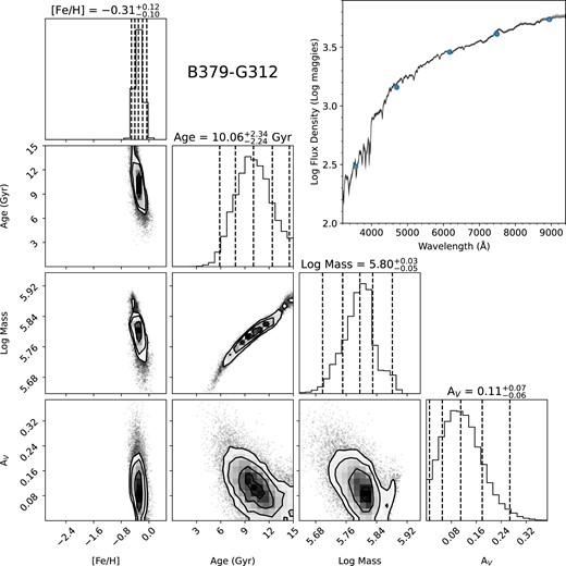
Posterior distributions of metallicity, age, mass, and reddenings for the M31 GC B379-G312 based on SDSS ugriz photometry and a CaT-based metallicity prior. In the top right, we plot the spectral energy distributions calculated by fsps for 256 points drawn at random from the posterior distribution in grey, the median colours of the posterior distribution as circles, and the observed photometry as error bars. We note that B379-G312 presents the best case for fitting its photometry, as it is bright, metal rich, and outside of the projected disc of M31.
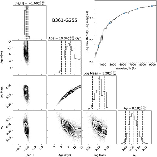
Posterior distributions of metallicity, age, mass, and reddenings for the M31 GC B361-G255 based on SDSS ugriz photometry and a CaT-based metallicity prior. In the top right, we plot the spectral energy distributions calculated by fsps for 256 points drawn at random from the posterior distribution in grey, the median colours of the posterior distribution as circles, and the observed photometry as error bars. Unlike B379-G312 plotted in Fig. 5, B361-G255 presents a more typical case for fitting its photometry, due to its median brightness and metal-poor nature.
Age and metallicity posteriors. Values provided median value of the posterior and the 68 per cent confidence interval. Column (1): GC name. Column (2): Right ascension in degrees. Column (3): Declination in degrees. Column (4): Metallicity prior from the strength of the CaT in dex. Column (5): V-band extinction prior from Schlegel et al. (1998) in magnitudes. Column (6): Mass posterior in log solar masses. Column (7): Age posterior in Gyr. Column (8): Metallicity posterior in dex. Column (9): V-band extinction posterior in magnitudes. Column (10): Photometry source. P10: Peacock et al. (2010), H14: Huxor et al. (2014), and SDSS: SDSS DR17 (Abdurro’uf et al. 2022). Column (11): Spectra source. C: Caldwell et al. (2009) and S: Sakari & Wallerstein (2016), Sakari et al. (2021), and Sakari & Wallerstein (2022). The full version of this table is provided in machine-readable form in the online Supporting Information.
| ID | RA | Dec. | [Fe/H]CaT | AVprior | Mass | Age | [Fe/H] | AV | Photo | Spectra |
|---|---|---|---|---|---|---|---|---|---|---|
| (deg) | (deg) | (dex) | (mag) | (log M⊙) | (Gyr) | (dex) | (mag) | |||
| (1) | (2) | (3) | (4) | (5) | (6) | (7) | (8) | (9) | (10) | (11) |
| B001-G039 | 9.9626 | 40.9696 | −0.53 ± 0.15 | 0.40 ± 0.20 | |$5.73_{-0.06}^{+0.04}$| | |$11.4_{-3.1}^{+2.5}$| | |$-0.64_{-0.11}^{+0.09}$| | |$0.89_{-0.09}^{+0.10}$| | P10 | C |
| B002-G043 | 10.0107 | 41.1982 | −2.16 ± 0.09 | 0.27 ± 0.14 | |$5.10_{-0.09}^{+0.04}$| | |$10.9_{-2.7}^{+2.7}$| | |$-2.15_{-0.09}^{+0.09}$| | |$0.29_{-0.04}^{+0.05}$| | P10 | C |
| B003-G045 | 10.0392 | 41.1849 | −1.47 ± 0.11 | 0.29 ± 0.15 | |$4.93_{-0.06}^{+0.10}$| | |$4.3_{-1.2}^{+3.1}$| | |$-1.47_{-0.09}^{+0.10}$| | |$0.58_{-0.13}^{+0.11}$| | P10 | C |
| B004-G050 | 10.0747 | 41.3779 | −0.57 ± 0.16 | 0.24 ± 0.12 | |$5.46_{-0.03}^{+0.03}$| | |$12.5_{-2.1}^{+1.7}$| | |$-0.76_{-0.08}^{+0.07}$| | |$0.25_{-0.07}^{+0.07}$| | P10 | C |
| B005-G052 | 10.0847 | 40.7329 | −0.68 ± 0.16 | 1.03 ± 0.51 | |$6.06_{-0.08}^{+0.03}$| | |$11.9_{-4.1}^{+2.2}$| | |$-0.72_{-0.12}^{+0.11}$| | |$0.44_{-0.11}^{+0.15}$| | P10 | C |
| ... | ... | ... | ... | ... | ... | ... | ... | ... | ... | ... |
A number of GCs from the Caldwell sample show surprisingly young age posteriors, given that the Caldwell sample of spectra were selected to be older than a couple of Gyr on the basis of their spectra between 3750 and 5400 Å (see section 5 of Caldwell et al. 2009). The lack of young GCs in both of the Caldwell and Sakari samples is supported by the lack of GC spectra with significant Paschen absorption, which is seen in stellar populations younger than ∼1 Gyr (e.g. Usher et al. 2019a). In the case of some GCs such as M009, the age is poorly constrained, with the posterior distribution spanning a wide range of ages (|$2.9_{-2.7}^{+8.8}$| Gyr in the case of M009 using the 16–84 per cent percentile confidence interval). However, a number of GCs are inconsistent with being as old as 5 Gyr at a 95 per cent level. As can be seen in Fig. 7, these GCs with apparently young ages are found at small galactocentric radii and have large priors on their extinctions. Thus, these GCs are found in the crowded centre of M31, where the effects of the age–extinction degeneracy are strongest and both photometry and spectroscopy are most likely to suffer from systematic uncertainty.

4.1 Comparison with previous measurements
A wealth of studies have examined the ages of GCs in M31 using a range of techniques. In the first class of studies, ages were constrained using resolved star colour–magnitude diagrams. Only B379-G312 has HST imaging deep enough to reach the main sequence turn-off and measure the age directly. For this GC (see Fig. 5), we find good agreement between our age measurement (|$10.1_{-2.2}^{+2.3}$| Gyr) and the colour–magnitude diagram-based literature values [|$10.0_{-1.0}^{+2.5}$| Gyr (Brown et al. 2004) and 11.0 ± 1.5 Gyr (Ma et al. 2010)]. Shallower HST imaging can be used to place lower limits on the ages of M31 GCs from the non-detection of a main sequence or from the presence of blue horizontal branch stars (e.g. Perina et al. 2011). Using the MIST isochrones (Choi et al. 2016) to estimate the brightness of the subgiant branch as a function of age and metallicity, we find no inconsistencies between the ages and metallicities we measure and the colour–magnitude diagrams in Perina et al. (2012) for the 34 GCs in common. Of the 12 GCs from Perina et al. (2012) with well-measured horizontal branch properties, all GCs with blue HBs are older than 11.6 Gyr except for B350-G162 (|$7.6_{-2.0}^{+4.0}$| Gyr), which is consistent with being old. Published colour–magnitude diagrams for PA06, PA53, PA54, and PA56 (Sakari et al. 2015) and EXT8 (Larsen, Romanowsky & Brodie 2021) all reveal blue horizontal branches, consistent with the old ages and low metallicities we measure.
Most studies of the ages of M31 GC have relied on integrated light. Some studies have measured line indices and then fitted stellar population models to the indices (e.g. Beasley et al. 2005; Puzia et al. 2005; Caldwell et al. 2011). Others have directly fitted stellar population models to spectra (e.g. Cezario et al. 2013; Colucci et al. 2014; Sakari et al. 2015; Chen et al. 2016), to photometry (e.g. Ma et al. 2009; Fan, de Grijs & Zhou 2010), or a combination thereof (Wang, Chen & Ma 2021).
In Fig. 8, we show a comparison between our ages and those from literature. In general, we see better agreement for GCs with low extinction priors [E(B − V) < 0.15 from Schlegel et al. 1998] than for GCs with higher extinction priors that are projected on to the disc of M31. This is unsurprising given the strong degeneracy between age and extinction for optical colours. While this degeneracy is usually considered in studies of young star clusters, it is often ignored in studies of old GCs where the observed extinction is assumed only to be due to the MW foreground. While this assumption is acceptable in galaxy haloes and in quiescent galaxies, it is not valid in actively star-forming galaxies.
![Comparison of our mcmc ages with ages from Beasley et al. (2005), Fan et al. (2010), Caldwell et al. (2011), Cezario et al. (2013), Colucci et al. (2014), Sakari et al. (2015), Chen et al. (2016), Wang et al. (2021), and Cabrera-Ziri et al. (in preparation). For each study, we show all GCs in common with high extinction priors [E(B − V) > 0.15 from Schlegel et al. 1998] as points and the GCs with low extinction priors [E(B − V) < 0.15] as circles with error bars. When literature age measurements are larger than 16 Gyr, we have plotted them at an age of 16 Gyr. The level of agreement varies between studies but in general we see good agreement.](https://oup.silverchair-cdn.com/oup/backfile/Content_public/Journal/mnras/528/4/10.1093_mnras_stae282/1/m_stae282fig8.jpeg?Expires=1750232585&Signature=oUqlFtc6fDklTHTuK2CcGMj4JF6gyQ1JhZ8OfS6laNSkAVRVXV537~vn9waUDePac~rSgiS0iLDbdhJGSJXq0LdS2KBjKZxJJFpQ5Vx8jkwCG-KEnBhas5RyiR~YCQAYBtTNy2VyaOlkCGeaOIzgulLCpqi52jm~9K335ZASYjKAno7Ve7RaCGredpTzoe4FJcC8pAqsTi0Mx2CsJ5yhMSuBAzif1oAr2mnDSSjNPE0xUghsKHoKRU~3i2IwNwAHItdJ3lTR24qji6U-E5Ba1SBnsZbic84CqWx1MzDUblNXUNfcEedcjb9ooFTC7eCufsEUt6VwfVezD3-4xpBe0g__&Key-Pair-Id=APKAIE5G5CRDK6RD3PGA)
Comparison of our mcmc ages with ages from Beasley et al. (2005), Fan et al. (2010), Caldwell et al. (2011), Cezario et al. (2013), Colucci et al. (2014), Sakari et al. (2015), Chen et al. (2016), Wang et al. (2021), and Cabrera-Ziri et al. (in preparation). For each study, we show all GCs in common with high extinction priors [E(B − V) > 0.15 from Schlegel et al. 1998] as points and the GCs with low extinction priors [E(B − V) < 0.15] as circles with error bars. When literature age measurements are larger than 16 Gyr, we have plotted them at an age of 16 Gyr. The level of agreement varies between studies but in general we see good agreement.
We compare our ages to ages measured by fitting stellar models to spectral indices (Beasley et al. 2005; Caldwell et al. 2011), by directly fitting stellar population models to spectra (Cezario et al. 2013; Colucci et al. 2014; Chen et al. 2016, Cabrera-Ziri et al. in preparation) and by fitting stellar population models to photometry (Fan et al. 2010). The level of agreement varies between studies, with the best agreement with Beasley et al. (2005), Caldwell et al. (2011), and Colucci et al. (2014) and the worst agreement with Fan et al. (2010) and Wang et al. (2021). Beasley et al. (2005) used both the Bruzual & Charlot (2003) and the Thomas, Maraston & Bender (2003) models to convert Lick index measurements to ages and metallicities. We find better agreement between our measurements and the Thomas et al. (2003)-based values of Beasley et al. (2005); we display the Thomas et al. (2003)-based ages in Fig. 8. Fan et al. (2010) fitted UBVRIJHK photometry with the Bruzual & Charlot (2003) models to derive ages and metallicities. A comparison of the Fan et al. (2010) metallicity measurements and our own reveals that they typically overestimate metallicities, which due to the age–metallicity degeneracy causes them to underestimate the ages. Caldwell et al. (2011) used EZAges (Graves & Schiavon 2008) to measure ages from Lick indices. Due to the effects of the horizontal branch at lower metallicities, Caldwell et al. (2011) only provide ages for GCs more metal rich than [Fe/H] = −0.95. Cezario et al. (2013) used full spectrum fitting and the Vazdekis et al. (2010) stellar population models to measure ages. Colucci et al. (2014) and Sakari et al. (2015) fitted their own stellar population models to high-resolution spectra to measure ages, metallicities, and abundances. Chen et al. (2016) measured ages using full spectral fitting both with the PEGASE–HR (Le Borgne et al. 2004) and the MILES (Vazdekis et al. 2010) stellar population models. The majority of PEGASE–HR-based ages are either significantly younger or older than our age measurements, while the MILES-based ages show better agreement; we display the MILES-based ages in Fig. 8. Wang et al. (2021) used a random forest classifier to derive ages and metallicities from Lick indices and ugriz photometry. They find ages of 6–8 Gyr for virtually all M31 GCs, inconsistent with our measurements and most other literature values. Cabrera-Ziri et al. (in preparation) used alf (Conroy & van Dokkum 2012; Choi et al. 2014; Conroy, Graves & van Dokkum 2014; Conroy et al. 2018; Cabrera-Ziri & Conroy 2022) to fit spectra to measure ages, metallicities, and abundances while accounting for the possibility of a hot horizontal branch. While we see agreement for many GCs, most of Cabrera-Ziri et al. (in preparation) age measurements are a couple of Gyr older than ours.
4.2 Age–metallicity distributions
In Fig. 9 we show the age–metallicity distributions of GCs associated with different components of M31, while in Table 2 we give the median ages and metallicities for each of the components. For GCs projected on to the disc of M31, which are based on the Caldwell et al. (2011) spectra and Peacock et al. (2010) photometry and have relatively broad extinction priors, we see a wide range of ages and metallicities. The wide range of ages is likely due to the age–extinction degeneracy. For GCs in the inner halo of M31 – not projected on to the disc on M31 but within 20 kpc in projection – which are based on Caldwell et al. (2011) spectra and Peacock et al. (2010) photometry and have relatively narrow extinction priors – we see generally old ages. The outer halo, beyond a distance of 25 kpc in projection and based on the Sakari et al. spectra and a mix of PAndAS and SDSS photometry, also shows old ages. Finally, the GCs associated with the dwarf elliptical NGC 205 show low metallicities. Four of the NGC 205 GCs show old ages but the fifth, B330-G056, shows evidence for a younger age (|$3.8_{-2.6}^{+3.9}$| Gyr).
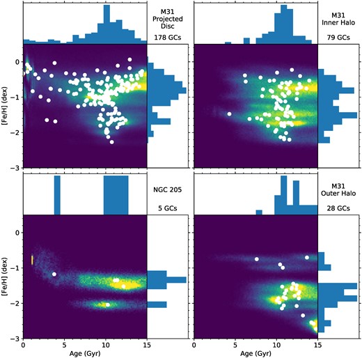
Age–metallicity posterior distributions for M31 GCs based on photometry assuming a bimodal extinction prior. The 2D histograms show the sum of the individual age–metallicity posterior distributions, while the white circles and the 1D histograms show the medians of the age and metallicity posteriors for each GC. In the top left panel, we show GCs projected on to the disc of M31. In the top right panel, we show GCs in the inner halo of M31 (projected galactocentric distances <20 kpc). In the bottom right panel, we show GCs in the outer halo of M31 (projected galactocentric distances >25 kpc). In the bottom left panel, we show GCs associated with the M31 satellite galaxy NGC 205. For the outer halo subsample, the ages and metallicities are on the Sakari et al. spectra and a mix of SDSS ugriz and PAndAS gi photometry; for the other subsamples, they are based on the Caldwell et al. (2011) spectra and the Peacock et al. (2010) SDSS ugriz photometry.
Population age and metallicity medians from this study and from Usher et al. (2019b). (1) Population name. (2) Median age in Gyr. (3) Median metallicity in dex. (4) Number of GCs.
| Population | Age | [Fe/H] | N |
|---|---|---|---|
| (Gyr) | (dex) | ||
| (1) | (2) | (3) | (4) |
| Combined | |$10.7_{-0.2}^{+0.2}$| | |$-1.00_{-0.01}^{+0.01}$| | 290 |
| Projected disc | |$10.3_{-0.3}^{+0.3}$| | |$-0.84_{-0.02}^{+0.02}$| | 178 |
| Inner halo | |$10.9_{-0.4}^{+0.4}$| | |$-1.22_{-0.03}^{+0.03}$| | 79 |
| Outer halo | |$12.5_{-0.5}^{+0.5}$| | |$-1.77_{-0.03}^{+0.03}$| | 28 |
| NGC 205 | |$10.8_{-1.1}^{+1.2}$| | |$-1.43_{-0.06}^{+0.07}$| | 5 |
| Smooth halo | |$12.4_{-0.8}^{+0.7}$| | |$-1.8_{-0.04}^{+0.04}$| | 16 |
| Ambiguous | |$11.2_{-1.1}^{+1.2}$| | |$-1.57_{-0.07}^{+0.06}$| | 5 |
| Substructure | |$11.3_{-1.0}^{+1.1}$| | |$-1.98_{-0.08}^{+0.09}$| | 7 |
| Ambiguous + substructure | |$11.3_{-0.7}^{+0.8}$| | |$-1.63_{-0.07}^{+0.06}$| | 12 |
| MW | |$11.7_{-0.6}^{+0.5}$| | |$-1.20_{-0.04}^{+0.04}$| | 65 |
| NGC 1407 | |$11.9_{-0.3}^{+0.3}$| | |$-0.60_{-0.02}^{+0.02}$| | 213 |
| NGC 3115 | |$10.9_{-0.4}^{+0.4}$| | |$-0.72_{-0.03}^{+0.03}$| | 116 |
| NGC 3377 | |$8.0_{-0.4}^{+0.5}$| | |$-0.80_{-0.06}^{+0.06}$| | 82 |
In line with the previously observed (Galleti et al. 2009; Caldwell et al. 2011; Sakari & Wallerstein 2022) metallicity gradient for M31 GCs, we see the range of metallicities shift to lower metallicities and the fraction of metal-poor GCs increase as we go out from the centre of M31. Using the commonly used gmm code of Muratov & Gnedin (2010), the projected disc and inner halo populations as well as the combined sample all show significant (p ≤ 0.01 as well as a negative kurtosis and well-separated peaks) evidence for bimodality, while the outer halo sample is too small to reliably use gmm. Pfeffer et al. (2023) discuss the emergence of GC metallicity bimodality in the context of GC formation and destruction, showing that in high-mass galaxies like M31, the relative lack of GCs at intermediate metallicities is likely due to these GCs being preferentially disrupted rather than a deficit of cluster formation.
We also see a positive age gradient, with GCs projected on to the disc having younger ages and the GCs in the outer halo having older ages, although it is unclear whether this is driven by the larger age uncertainties at smaller radii. The less constraining the observations are, the more the age posterior will resemble the prior, with our uniform prior having a median age of 7.5 Gyr. Caldwell & Romanowsky (2016) divided M31 GCs up by metallicity into three components. The most metal-poor ([Fe/H] < −1.5) component and the intermediate-metallicity (−1.5 < [Fe/H] < −0.4) component show consistent ages (|$10.9_{-0.3}^{+0.4}$| and |$10.4_{-0.3}^{+0.3}$| Gyr, respectively), while the most metal-rich component ([Fe/H] > −0.4) shows a slightly younger median age (|$8.3_{-1.6}^{+1.5}$| Gyr). We note that all but 3 of the 26 metal-rich GCs have large reddening priors, so we cannot rule out that the younger age median for the most metal-rich GCs is due to their larger uncertainties.
In the projected disc sample, we see a lack of GCs with metallicities [Fe/H] ∼ −1.2 with median age posteriors older than 11 Gyr that are present at higher or lower metallicities. It is unclear whether this is driven by the larger age uncertainties in this metallicity range compared to lower metallicity GCs or a genuine lack of relatively old GCs in this metallicity range. The most metal-poor and metal-rich GCs show the oldest ages, with some age posteriors having medians older than the age of the Universe. Under the naive expectation that the metallicity of a galaxy increases over time, the most metal-poor GCs should be the oldest. However, it is also plausible that such metal-poor GCs formed later, either in a less massive galaxy or, less likely, in a galaxy that has recently accreted a large amount of near-pristine gas. We also note that the three most metal-poor GCs in M31, all found in the outer halo, lie in a regime − more metal poor than any GCs in the MW and similar to the faintest ultra-faint galaxies (e.g. Simon 2019) – where stellar evolution models and stellar population models are not as well tested. The old ages of the most metal-rich GCs are more puzzling as the expectation is that more metal-rich GC should be younger than GCs that formed in the same progenitor. Although many of the lower metallicity GCs likely formed later in lower mass progenitors, it is unlikely that no lower metallicity GCs formed in and survived from the progenitor(s) of the metal-rich GCs. We note than many of these old GCs have large extinction priors and lie at small galactocentric radii where the systematic and statistical uncertainty of both the spectra and photometry is higher (see Fig. 7).
If we had systematically underestimated the CaT metallicity priors, we would systematically overestimate the ages. Due to the low resolution of the spectra used, the CaT metallicity prior is less reliable at these high metallicities. However, Usher et al. (2019b) also saw a trend of increasing age with metallicity for the most metal-rich GCs in NGC 1407 and NGC 3115 (see Fig. 11) suggesting that this issue is not due to the lower resolution spectra. Since the CaT metallicity is sensitive to the α-element abundance in general and the Ca abundance in particular, differences in the [Ca/Fe] ratio of high-metallicity M31 GCs to the MW GCs used to calibrate the CaT–[Fe/H] relation could introduce a bias. However, measurements of the α-elements in M31 GCs (e.g. Colucci et al. 2014; Sakari et al. 2016; Larsen et al. 2022) find similar ratios to MW GCs, although only a handful of near-solar metallicity GCs have been studied in M31.
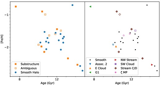
Age–metallicity distribution of outer halo GCs. In the left panel, we show the GCs associated with the smooth halo by Mackey et al. (2019) as circles and GCs associated with substructure as filled squares. GCs classified as ambiguous by Mackey et al. (2019) are denoted by open squares. The youngest and most metal-rich GCs are more likely to be associated with substructure than the smooth halo, in line with the predictions of Hughes et al. (2019). In the right panel, we show GCs associated with the smooth halo as black points, while the GCs associated with substructure are shown as coloured polygons. The colour and shape of these GCs correspond to their classification by Mackey et al. (2019) with GCs with ambiguous classifications having open symbols. Unfortunately, there are too few GCs associated with each substructure to robustly look for different age–metallicity relationships.
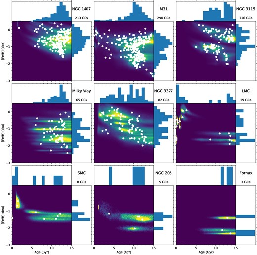
GC age–metallicity posterior distributions for the galaxies studied in this work (M31 and NGC 205) and the galaxies from Usher et al. (2019b). The galaxies are ordered by stellar mass using masses from Forbes et al. (2017) for the three SLUGGS galaxies, from Conn et al. (2012) for M31, from Bland-Hawthorn & Gerhard (2016) for the MW, and from McConnachie (2012) for the Local Group dwarf galaxies. As in Fig. 9, the 2D histograms show the sum of the individual age–metallicity posterior distributions, while the white circles and the 1D histograms show the medians of the age and metallicity posteriors for each GC.
Additionally, if the stellar population models we utilize predict too blue of a spectral energy distribution for a given age and metallicity, the resulting age constraint will be biased to older ages. More subtly, the combination of incorrectly predicted colours and poorly constrained reddening could lead to an older age and lower reddening being a better fit than the correct age and reddening. Again, differences in chemistry between the models and the data could produce colour differences. The models we utilize have a scaled solar abundance pattern, while GCs generally have α-element-enhanced abundances and typically show internal spreads in the abundances of light elements, with some stars showing enhanced He, N, and Na and depleted C and O (see review by Bastian & Lardo 2018). Coelho et al. (2007), Lee et al. (2009), and Choi, Conroy & Johnson (2019) all find that an α-element-enhanced population is bluer in shorter wavelength colours such as (u − g) and (g − r) and redder in longer wavelength colours like (r − i) and (i − z). Using models also based on the MIST isochrones and MILES stellar library, Choi et al. (2019) find that α-element-enhanced models are a better fit to the colours of massive early-type galaxies than scaled solar models, while noting that the abundances of C and N also significantly affect the colours of an old, metal-rich population. Chantereau, Usher & Bastian (2018) modelled the effects of He and of enhanced N and Na with depleted C and O populations. He-enhanced populations are bluer in all optical colours (see also Chung, Yoon & Lee 2017), while N- and Na-enhanced and C- and O-depleted populations have the same (u − g) colours as solar abundance models but bluer (g − r), (r − i), and (i − z). We note that the effects of abundance variations on colour are generally larger in older and higher metallicity populations since the effects are stronger in cooler stars (e.g. Lee et al. 2009). Further work is required to understand what effect different abundance ratios have on age estimates.
We note that there are larger systematic uncertainties in comparing ages at different metallicities than comparing ages at the same metallicity. Given the larger systematic uncertainties at the extremes of the metallicity distribution and the larger statistical uncertainties for GCs in the projected disc, we do not attach any significance to the variation of the age of the oldest GCs with metallicity.
For GCs in the outer halo, we used the association of Mackey et al. (2019) between halo substructure and GCs to compare the GCs associated with the smooth halo with those associated with substructure. As seen in the left panel of Fig. 10, although there are old and extremely metal-poor GCs associated with both the smooth halo and substructure, GCs associated with halo substructure extend to younger ages than those associated with the smooth halo. The situation with metallicity is more complex. Although the substructure and smooth halo GCs cover a similar range of metallicities and have similar medians, 2 of the 7 GCs that are securely identified with substructure and 1 of the 5 ambiguous GCs are more metal rich than [Fe/H] = −1.25, while only 1 of the 16 smooth halo GCs is above this metallicity. In Table 2, we give the medians of each of the populations. The most metal-rich smooth halo GC in our sample, PA-17, is older than the substructure GCs of similar metallicity. That GCs with substructure and ambiguous classifications have higher metallicities than those classified as part of the smooth halo has been previously noted by Sakari & Wallerstein (2022). The younger ages and higher metallicities of some GCs associated with substructure support the predictions of Hughes et al. (2019) where the substructured halo has been more recently accreted than the smooth halo. In the right panel of Fig. 10, we show the association of the substructure GCs with each halo feature; unfortunately, there are too few GCs associated with each substructure to robustly study the age–metallicity relationship of each substructure.
We can compare the age–metallicity distribution of M31 GCs with those of the galaxies studied by Usher et al. (2019b) in Fig. 11. We note that although the technique used by Usher et al. (2019b) is the same as in this paper, the GC selection and data quality differ between M31 and the Usher et al. (2019b) galaxies. As noted by Usher et al. (2019a), the CaT is not a reliable metallicity indicator at ages younger than a couple of Gyr when stages of stellar evolution other than the red giant branch or the red clump dominate the light in the CaT spectral region. However, as noted by Usher et al. (2019b) due to weaker sensitivity of colour to metallicity at younger ages, our method still provides young ages for these star clusters. For the giant galaxies, M31 GCs are slightly younger than those of NGC 1407 and the MW, similar in age to those of NGC 3115 and older than those of NGC 3377 while being more metal poor than those of the three SLUGGS galaxies and more metal rich than those of the MW. For the dwarf galaxies, NGC 205 GCs show similar ages and metallicities to the old and intermediate-age GCs in the similar mass Small Magellanic Cloud (SMC).
Although we defer a detailed and quantitative discussion of M31’s formation and assembly history to future work, we can discuss M31 GC system in a qualitative manner similar to Usher et al. (2019b). That most of M31 GCs are old suggests that M31 formed most of its stellar mass early, in line with the observed star formation history of M31’s disc and spheroid (e.g. Brown et al. 2008; Bernard et al. 2015; Williams et al. 2017). The lack of clear branches in age–metallicity space does not have a strong implication on the assembly history of M31 given our large age uncertainties. As can be seen in Fig. 11, with similar quality data we do not see the bifurcation of the MW GCs into the older in situ branch and a younger accreted branch that more precise ages relieve (Forbes & Bridges 2010; Leaman et al. 2013). Comparing M31 to the galaxies studied in Usher et al. (2019b), the similarities between the age and metallicity distributions of M31, NGC 1407, and the MW suggest some commonality in the assembly history of these galaxies compared to the extended formation of NGC 3377 and the bimodality of NGC 3115.
5 SUMMARY
Using the strength of the near-infrared CaT spectral feature, we have measured the metallicity of a large number of GCs in M31. In line with previous work (e.g. Sakari & Wallerstein 2016; Usher et al. 2019a), we find that the CaT is a reliable measure of metallicity, although its reliability declines at high metallicity and at the lower spectral resolution of the Caldwell et al. (2009) Hectospec spectra. We used these metallicities as priors when fitting optical photometry with stellar population models to measure the ages, metallicities, and masses of the GCs. Due to the strong degeneracy between extinction and age, the ages of GCs projected on to the disc of M31 are less reliable than those in the halo of M31. We find good agreement between our age measurements with most but not all literature studies. Most of the GCs projected on to the disc and virtually all halo GCs are old (consistent with ages >10.5 Gyr, formation redshifts z > 2). The distribution of GC ages and metallicities is similar but not identical to galaxies with a similar stellar mass. The old ages of the majority of M31 GCs suggest that M31 formed much of its stellar mass early, in line with observations of the field star formation history. In the outer halo, we find that the most metal-rich and youngest GCs are more likely to be associated with substructure rather than the smooth halo, in line with the predictions of Hughes et al. (2019).
The technique used in this paper of combining photometry with a prior from spectroscopy is likely not the best way of measuring the ages of M31 GCs where high S/N optical spectra are available (see Cabrera-Ziri et al., in preparation). Instead, it serves as a test of a technique suitable for more distant galaxies. Upcoming highly multiplexed red and near-infrared spectrographs, such as Multi-Object Optical and Near-infrared Spectrograph (MOONS) (Cirasuolo et al. 2014; Taylor et al. 2018) on the Very Large Telescope, will allow large numbers of extragalactic GCs to be observed efficiently. Like other techniques that rely on photometry, our method suffers from the age–extinction degeneracy and will perform worse when there is not a strong prior on extinction, such as in or near areas of active star formation. In addition, spectra, even when only available in the red or near-infrared, do provide some age information. This technique should be refined either by fitting the spectra with stellar population models and using that age–metallicity posterior as a prior when fitting the photometry or by simultaneously fitting the photometry and spectroscopy with a stellar population model.
ACKNOWLEDGEMENTS
We thank the anonymous referee for their helpful comments, which improved the manuscript. We also wish to thank Joel Pfeffer for useful discussions. CU acknowledges the support of the Swedish Research Council, Vetenskapsrådet. This study was supported by the Klaus Tschira Foundation. We wish to thank Charli Sakari for making her spectra available.
This work made use of numpy (van der Walt, Colbert & Varoquaux 2011), scipy (Jones, Oliphant & Peterson 2001), matplotlib (Hunter 2007), and corner (Foreman-Mackey 2016) as well as astropy, a community-developed core python package for astronomy (Astropy Collaboration 2013). The CaT fitting code of Usher et al. (2019a) relies on ppxf (Cappellari & Emsellem 2004; Cappellari 2017).
Funding for the SDSS-IV has been provided by the Alfred P. Sloan Foundation, the U.S. Department of Energy Office of Science, and the Participating Institutions. SDSS-IV acknowledges support and resources from the Center for High Performance Computing at the University of Utah. The SDSS website is www.sdss.org. SDSS-IV is managed by the Astrophysical Research Consortium for the Participating Institutions of the SDSS Collaboration including the Brazilian Participation Group, the Carnegie Institution for Science, Carnegie Mellon University, Center for Astrophysics| Harvard & Smithsonian, the Chilean Participation Group, the French Participation Group, Instituto de Astrofísica de Canarias, the Johns Hopkins University, Kavli Institute for the Physics and Mathematics of the Universe (IPMU)/University of Tokyo, the Korean Participation Group, Lawrence Berkeley National Laboratory, Leibniz Institut für Astrophysik Potsdam (AIP), Max-Planck-Institut für Astronomie (MPIA, Heidelberg), Max-Planck-Institut für Astrophysik (MPA, Garching), Max-Planck-Institut für Extraterrestrische Physik (MPE), National Astronomical Observatories of China, New Mexico State University, New York University, University of Notre Dame, Observatário Nacional/MCTI, the Ohio State University, Pennsylvania State University, Shanghai Astronomical Observatory, United Kingdom Participation Group, Universidad Nacional Autónoma de México, University of Arizona, University of Colorado Boulder, University of Oxford, University of Portsmouth, University of Utah, University of Virginia, University of Washington, University of Wisconsin, Vanderbilt University, and Yale University.
DATA AVAILABILITY
The Caldwell et al. (2009) spectra are available from https://oirsa.cfa.harvard.edu/signature_program/. The Sakari & Wallerstein (2016, 2022) and Sakari et al. (2021) spectra are available upon request from Charli Sakari. The Peacock et al. (2010) and Huxor et al. (2014) photometry was taken from those papers; the remaining SDSS DR17 (Abdurro’uf et al. 2022) photometry is available from http://skyserver.sdss.org/dr17.
