


ABSTRACT
High redshift blazars are among the most powerful non-explosive sources in the Universe and play a crucial role in understanding the evolution of relativistic jets. To understand these bright objects, we performed a detailed investigation of the multiwavelength properties of 79 γ-ray blazars with redshifts ranging from z = 2.0 to 2.5, using data from Fermi LAT, Swift XRT/UVOT, and NuSTAR observations. In the γ-ray band, the spectral analysis revealed a wide range of flux and photon indices, from 5.32 × 10⁻¹⁰ to 3.40 × 10⁻⁷ photon cm−2 s−1 and from 1.66 to 3.15, respectively, highlighting the diverse nature of these sources. The detailed temporal analysis showed that flaring activities were observed in 31 sources. Sources such as 4C+71.07, PKS 1329-049, and 4C + 01.02, demonstrated significant increase in the γ-ray luminosity and flux variations, reaching peak luminosity exceeding 1050 erg s−1. The temporal analysis extended to X-ray and optical/ultraviolet (UV) bands, showed clear flux changes in some sources in different observations. The time-averaged properties of high redshift blazars were derived through modeling the spectral energy distributions with a one-zone leptonic scenario, assuming the emission region is within the broad-line region (BLR) and the X-ray and γ-ray emissions are due to inverse Compton scattering of synchrotron and BLR-reflected photons. This modeling allowed us to constrain the emitting particle distribution, estimate the magnetic field inside the jet, and evaluate the jet luminosity, which is discussed in comparison with the disc luminosity derived from fitting the excess in the UV band.
1 INTRODUCTION
Blazars are jetted active galactic nuclei (AGN) and are among the most powerful persistent sources of electromagnetic radiation in the universe. Current unification theories assumes that blazars are a subtype of AGNs with jets oriented at a small angle relative to the observer’s line of sight (Urry & Padovani 1995). Their emission is believed to be primarily powered by the accretion of matter into supermassive black holes (Blandford & Znajek 1977) and exhibit extreme characteristics, such as high-amplitude and short-time-scale variability, core dominance, superluminal motion, and significant optical polarization. Blazars are typically grouped into two main groups based on the presence of emission lines in their spectra (Urry & Padovani 1995): BL Lacertae objects (BL Lacs), which have weak or absent emission lines, and flat spectrum radio quasars (FSRQs), which display strong emission lines.
The non-thermal emission from the jets of blazars is observable across almost all accessible bands of the electromagnetic spectrum (Padovani et al. 2017) up to high energy (HE; >100 MeV) and very high energy (VHE; >100 MeV) γ-ray bands. Their broad-band spectral energy distribution (SED) typically shows two broad humps. The lower-energy component, from the radio to the optical/X-ray band, is generally attributed to the synchrotron emission of electrons. The frequency of the synchrotron peak (νp) serves as a criterion to further classify blazars: as low synchrotron peaked sources (LSPs or LBLs), intermediate synchrotron peaked sources (ISPs or IBLs), or high synchrotron peaked sources (HSPs or HBLs) when νp < 1014 Hz, 1014 Hz < νp < 1015 Hz, and νp > 1015 Hz, respectively (Padovani & Giommi 1995; Abdo et al. 2010). The origin of the second component, however, remains a subject of debate. In leptonic scenarios, this second peak is interpreted as the result of inverse Compton scattering of low-energy photons, which may be of internal or external origin. In the synchrotron self-Compton (SSC) models (Ghisellini, Maraschi & Treves 1985; Maraschi, Ghisellini & Celotti 1992; Bloom & Marscher 1996), it is the synchrotron photons that are upscattered through inverse Compton processes. On the other hand, external inverse Compton (EIC) scenarios (e.g. Sikora, Begelman & Rees 1994) suggest that the photons originate outside the jet, coming directly from the accretion disc (Dermer, Schlickeiser & Mastichiadis 1992; Dermer & Schlickeiser 1994), or they may be reprocessed by the broad-line region (BLR; Sikora, Begelman & Rees 1994), or emitted from the torus (Błażejowski et al. 2000). In Bégué et al. (2023), a novel approach for fitting the blazar SED utilizing convolutional neural networks is introduced which allows self-consistent modeling, enabling a more detailed interpretation of the observed results.
In alternative models such as the hadronic or lepto-hadronic scenarios, the second spectral bump is assumed to be from the synchrotron emission of ultra-HE protons or from the decay of secondary particles produced during hadronic interactions (Mannheim & Biermann 1989; Mannheim 1993; Mücke & Protheroe 2001; Mücke et al. 2003; Böttcher et al. 2013; Petropoulou & Mastichiadis 2015; Gasparyan, Bégué & Sahakyan 2022). Interest in these models has increased, particularly after establishing a potential link between blazars and VHE neutrinos, following the association of TXS 0506 + 056 with the IceCube-170922A neutrino event (Padovani et al. 2018; IceCube Collaboration 2018a, b), and the detection of multiple neutrino events concurrent with the active phase of PKS 0735 + 178 in optical/ultraviolet (UV), X-ray, and γ-ray bands (Sahakyan et al. 2023a). These multimessenger observations have started extensive discussions, with various models being applied to explain the multimessenger observations of blazars (Ansoldi et al. 2018; Keivani et al. 2018; Murase, Oikonomou & Petropoulou 2018; Padovani et al. 2018; Sahakyan 2018; Cerruti et al. 2019; Gao et al. 2019; Righi, Tavecchio & Pacciani 2019; Sahakyan 2019; Gasparyan, Bégué & Sahakyan 2022).
The emission from blazars is highly beamed, and their bolometric luminosity can exceed 1048 erg s−1, allowing them to be observed even at very high redshifts (e.g. see Ackermann et al. 2017; Sahakyan et al. 2020). These distant blazars are particularly interesting, as their study offers insights into the formation and evolution of supermassive black holes, relativistic jets, and the connections between accretion discs and jets. Moreover, their γ-ray emission is important for probing the early universe; γ-ray emission from distant blazars undergoes attenuation via γγ absorption when interacting with extragalactic background light (EBL) photons, thereby enabling observations that can constrain the EBL’s density.The multiwavelength properties of distant blazars have been extensively studied in a number of publications (e.g. see Pacciani et al. 2012; Paliya 2015; Paliya et al. 2015, 2016, 2017, 2019; D’Ammando & Orienti 2016; Orienti et al. 2016; Marcotulli et al. 2017; Liao et al. 2019; Li et al. 2020; Sahakyan et al. 2020; Sahakyan, Harutyunyan & Israyelyan 2023b). In Sahakyan et al. (2020), the origin of emission from the most distant blazars detected in the HE γ-ray band (z > 2.5) was investigated analysing data in the optical/UV, X-ray, and γ-ray bands. From the temporal evolution of emission in these bands, flaring periods were identified when the luminosity substantially increased. Their broad-band emission was modeled using one-zone SSC and EIC models, assuming that the external photons are infrared (IR) photons from the dusty torus [see Arsioli & Chang (2018) for a discussion on the contribution of different external fields in shaping the HE emission of LSPs]. As a result, the parameters that characterize the particle emission and jet in these distant blazars were estimated.
In this work, we expand the study by Sahakyan et al. (2020) to γ-ray emitting blazars which have estimated redshifts that are in the range of z = 2.0–2.5. A prolonged observation period of ∼14 yr enables a comprehensive investigation of emissions from these sources across optical/UV, X-ray, and γ-ray bands as well as to perform detailed spectral and temporal analysis. Using the analysed data broad-band SEDs for a substantial number of sources were constrained and modeled which allows for a systematic comparison of blazar emission parameters at varying distances, which, in turn, could enhance our understanding of these brightest objects.
The structure of the paper is as follows: Section 2 introduces the sample of sources under consideration; Section 3 details the data analysis methodology; Section 4 presents the results of the data analysis; Section 5 discusses the modeling of broad-band SEDs; and Section 6 outlines the modeling results. Finally, the conclusions are summarized in Section 7.
2 SOURCE SAMPLE
The fourth catalogue of AGNs detected by the Fermi Large Area Telescope (Fermi-LAT; Ajello et al. 2022) contains 3814 blazars, among which 792 are FSRQs, 1458 are BL Lacs, and 1493 are blazar candidates of uncertain type (BCUs). The most distant blazar, GB 1508 + 5714, is at z = 4.31. A small fraction of the blazars, 79 (2.07 per cent), have a redshift between 2.0 < z < 2.5, and these are the ones selected for the current study (the source sample). This group includes 64 FSRQs, 9 BL Lacs, and 6 BCUs. The BL Lacs generally have redshifts lower than z = 2.1, with the exception of SDSS J145059.99 + 520111.7, which is at z = 2.47. Among the BL Lacs, there are three LBLs, four IBLs, and only two HBLs. The FSRQs have a more homogeneous redshift distribution, being observed at almost all redshifts; the most distant FSRQ in the sample is S5 1053 + 70 at z = 2.49. BCUs, which exhibit characteristics similar to blazars but lack reliable optical associations, have been observed across a range of redshifts. For instance, 4FGL J1139.0+4033 (CRATES J113903 + 403303) has been observed at z = 2.36, while 4FGL J1003.4+0205 (SDSS J100326.63 + 020455.6) is located at z = 2.08. In Sahakyan, Vardanyan & Khachatryan (2022a) BCUs were classified by training machine-learning algorithms on the γ-ray properties of FSRQs and BL Lacs. According to those criteria, four BCUs from our sample show probability similar to FSRQs (CRATES J113903+403303, MG4 J162750+4802, TXS 2315+189, and SDSS J120542.82+332146.9), one to BL Lacs (SDSS J100326.63+020455.6) and one (SDSS J120542.82 + 332146.9) can not be classified.
In summary, the source sample considered in this study comprises 79 objects. In Table 1, the three leftmost columns list these sources along with their 4FGL names and classes. The spatial distribution of these blazars in Galactic coordinates is depicted in the Hammer–Aitoff projection shown in Fig. 1. For completeness, this figure also includes blazars with redshifts greater than z > 2.5, as reported by Sahakyan et al. (2020).
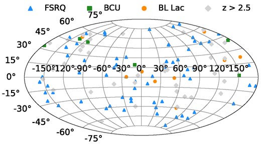
Hammer–Aitoff projection in Galactic coordinates showing the distribution of γ-ray blazars with redshifts above z > 2.0. BL Lacs within the redshift range 2.0 ≤ z ≤ 2.5 are represented by circles, FSRQs are depicted by triangles, BCUs by squares, and blazars with redshifts z > 2.5 are shown by diamonds.
The table shows the source sample, detailing the outcomes of the γ-ray analysis.
| Object | 4FGL name | Class | αp/α | β | Flux | Luminosity | z |
|---|---|---|---|---|---|---|---|
| S5 1053 + 70 | 4FGL J1056.8 + 7012 | FSRQ | 2.70 ± 0.08 | 0.23 ± 0.08 | 1.92 ± 0.55 | 6.51 ± 0.46 | 2.492 |
| PMN J1344-1723 | 4FGL J1344.2-1723 | FSRQ | 2.03 ± 0.04 | 0.14 ± 0.02 | 1.68 ± 0.14 | 9.79 ± 0.5 | 2.490 |
| SDSS J145059.99 + 520111.7 | 4FGL J1450.8 + 5201 | BLL | 2.11 ± 0.08 | 0.09 ± 0.04 | 0.64 ± 0.16 | 3.79 ± 0.44 | 2.471 |
| PKS 1915–458 | 4FGL J1919.4-4550 | FSRQ | 3.15 ± 0.12 | - | 1.47 ± 0.18 | 2.19 ± 0.26 | 2.470 |
| PKS 0226–559 | 4FGL J0228.3-5547 | FSRQ | 2.24 ± 0.02 | 0.11 ± 0.01 | 5.04 ± 0.18 | 22.1 ± 0.49 | 2.464 |
| S3 2214 + 30 | 4FGL J2216.8 + 3103 | FSRQ | 2.66 ± 0.28 | 0.33 ± 0.19 | 0.26 ± 0.12 | 0.89 ± 0.28 | 2.462 |
| PKS 2315–172 | 4FGL J2318.6-1657 | FSRQ | 2.21 ± 0.01 | - | 0.20 ± 0.00 | 0.76 ± 0.02 | 2.462 |
| PKS 0601–70 | 4FGL J0601.1-7035 | FSRQ | 2.27 ± 0.03 | 0.09 ± 0.02 | 3.51 ± 0.17 | 11.22 ± 0.39 | 2.409 |
| B2 1436 + 37B | 4FGL J1438.9 + 3710 | FSRQ | 2.33 ± 0.05 | 0.10 ± 0.03 | 1.88 ± 0.14 | 5.24 ± 0.27 | 2.401 |
| 2MASS J16561677-33021271 | 4FGL J1656.3-3301 | FSRQ | 2.94 ± 0.11 | 0.32 ± 0.09 | 3.47 ± 0.72 | 6.68 ± 0.70 | 2.400 |
| MG1 J173624 + 0632 | 4FGL J1736.6 + 0628 | FSRQ | 2.67 ± 0.08 | - | 1.58 ± 0.21 | 2.90 ± 0.39 | 2.387 |
| TXS 1645 + 635 | 4FGL J1645.6 + 6329 | FSRQ | 2.46 ± 0.06 | 0.13 ± 0.04 | 1.41 ± 0.12 | 3.28 ± 0.2 | 2.379 |
| PKS B1149-084 | 4FGL J1152.3-0839 | FSRQ | 2.33 ± 0.04 | 0.11 ± 0.02 | 2.79 ± 0.19 | 7.9 ± 0.38 | 2.370 |
| S5 0212 + 73 | 4FGL J0217.4 + 7352 | FSRQ | 2.93 ± 0.04 | 0.15 ± 0.03 | 3.52 ± 0.17 | 5.56 ± 0.2 | 2.367 |
| B2 0552 + 39A | 4FGL J0555.6 + 3947 | FSRQ | 2.67 ± 0.00 | 0.15 ± 0.00 | 3.98 ± 0.02 | 7.5 ± 0.02 | 2.365 |
| CRATES J113903 + 403303 | 4FGL J1139.0 + 4033 | BCU | 2.73 ± 0.09 | - | 1.13 ± 0.18 | 1.90 ± 0.30 | 2.360 |
| B2 2112 + 28B | 4FGL J2114.8 + 2831 | FSRQ | 2.50 ± 0.21 | 0.42 ± 0.18 | 0.33 ± 0.15 | 1.54 ± 0.36 | 2.345 |
| PKS 2149–306 | 4FGL J2151.8-3027 | FSRQ | 2.86 ± 0.03 | 0.17 ± 0.03 | 7.01 ± 0.21 | 10.85 ± 0.3 | 2.345 |
| PKS 1430–178 | 4FGL J1433.0-1801 | FSRQ | 2.71 ± 0.02 | 0.30 ± 0.01 | 0.60 ± 0.03 | 1.53 ± 0.1 | 2.331 |
| MG4 J162750 + 4802 | 4FGL J1627.3 + 4758 | BCU | 2.64 ± 0.16 | 0.11 ± 0.11 | 0.46 ± 0.16 | 0.96 ± 0.21 | 2.326 |
| PMN J0743-5619 | 4FGL J0743.0-5622 | FSRQ | 2.90 ± 0.19 | - | 1.01 ± 0.22 | 1.45 ± 0.32 | 2.319 |
| GB6 J0742 + 4900 | 4FGL J0742.1 + 4902 | FSRQ | 2.24 ± 0.09 | - | 0.46 ± 0.10 | 1.38 ± 0.30 | 2.312 |
| S3 0458–02 | 4FGL J0501.2-0158 | FSRQ | 2.29 ± 0.01 | 0.09 ± 0.01 | 10.80 ± 0.19 | 27.57 ± 0.4 | 2.291 |
| PMN J0157-4614 | 4FGL J0157.7-4614 | FSRQ | 2.26 ± 0.13 | 0.26 ± 0.09 | 0.55 ± 0.15 | 2.08 ± 0.24 | 2.287 |
| PKS 0726–476 | 4FGL J0728.0-4740 | FSRQ | 2.36 ± 0.24 | - | 0.45 ± 0.32 | 1.06 ± 0.75 | 2.282 |
| PKS 0420 + 022 | 4FGL J0422.8 + 0225 | FSRQ | 2.63 ± 0.19 | 0.37 ± 0.17 | 1.11 ± 0.24 | 1.95 ± 0.28 | 2.277 |
| PKS 2245–328 | 4FGL J2248.7-3235 | FSRQ | 2.67 ± 0.05 | - | 2.01 ± 0.14 | 3.23 ± 0.22 | 2.268 |
| PKS B2224 + 006 | 4FGL J2226.8 + 0051 | FSRQ | 2.98 ± 0.24 | 0.31 ± 0.10 | 0.92 ± 0.17 | 1.81 ± 0.32 | 2.262 |
| TXS 1322 + 479 | 4FGL J1324.9 + 4748 | FSRQ | 2.67 ± 0.07 | - | 1.09 ± 0.13 | 1.74 ± 0.21 | 2.260 |
| PKS 2244–37 | 4FGL J2247.5-3700 | FSRQ | 2.40 ± 0.20 | - | 0.19 ± 0.09 | 0.41 ± 0.19 | 2.252 |
| B2 0242 + 23 | 4FGL J0245.4 + 2408 | FSRQ | 2.67 ± 0.05 | - | 1.98 ± 0.16 | 3.09 ± 0.25 | 2.243 |
| 4C + 71.07 | 4FGL J0841.3 + 7053 | FSRQ | 2.81 ± 0.02 | 0.21 ± 0.02 | 10.68 ± 0.17 | 14.76 ± 0.23 | 2.218 |
| PKS 2022 + 031 | 4FGL J2025.2 + 0317 | FSRQ | 2.07 ± 0.06 | 0.09 ± 0.03 | 0.92 ± 0.13 | 4.03 ± 0.37 | 2.210 |
| MG2 J174753 + 2323 | 4FGL J1747.4 + 2330 | FSRQ | 2.79 ± 0.03 | 0.39 ± 0.03 | 0.80 ± 0.03 | 1.2 ± 0.03 | 2.203 |
| MG2 J153938 + 2744 | 4FGL J1539.6 + 2743 | FSRQ | 2.23 ± 0.06 | 0.05 ± 0.03 | 1.18 ± 0.13 | 3.12 ± 0.23 | 2.196 |
| S4 0917 + 44 | 4FGL J0920.9 + 4441 | FSRQ | 2.35 ± 0.02 | 0.15 ± 0.02 | 5.88 ± 0.35 | 17.97 ± 0.43 | 2.186 |
| PMN J2135-5006 | 4FGL J2135.3-5006 | FSRQ | 2.40 ± 0.05 | 0.10 ± 0.03 | 1.99 ± 0.13 | 3.92 ± 0.2 | 2.181 |
| OX 131 | 4FGL J2121.0 + 1901 | FSRQ | 2.14 ± 0.03 | 0.05 ± 0.01 | 2.68 ± 0.17 | 8.77 ± 0.38 | 2.180 |
| PMN J1959-4246 | 4FGL J1959.1-4247 | FSRQ | 2.16 ± 0.10 | 0.19 ± 0.06 | 0.88 ± 0.15 | 2.76 ± 0.26 | 2.174 |
| B3 1520 + 437 | 4FGL J1521.8 + 4338 | FSRQ | 3.00 ± 0.10 | - | 1.14 ± 0.15 | 1.32 ± 0.17 | 2.168 |
| TXS 2315 + 189 | 4FGL J2318.2 + 1915 | BCU | 2.60 ± 0.01 | - | 1.60 ± 0.03 | 2.43 ± 0.05 | 2.163 |
| PKS 0446 + 11 | 4FGL J0449.1 + 1121 | FSRQ | 2.37 ± 0.03 | 0.13 ± 0.02 | 6.25 ± 0.21 | 12.12 ± 0.34 | 2.153 |
| PKS 1329–049 | 4FGL J1332.0-0509 | FSRQ | 2.41 ± 0.02 | 0.16 ± 0.02 | 6.33 ± 0.18 | 11.57 ± 0.32 | 2.150 |
| PMN J2227 + 0037 | 4FGL J2227.9 + 0036 | BLL | 1.77 ± 0.11 | 0.15 ± 0.05 | 0.31 ± 0.10 | 3.79 ± 0.54 | 2.145 |
| TXS 2321–065 | 4FGL J2323.6-0617 | FSRQ | 2.32 ± 0.10 | 0.18 ± 0.06 | 0.87 ± 0.16 | 2.14 ± 0.24 | 2.144 |
| PMN J1402-3334 | 4FGL J1402.6-3330 | FSRQ | 3.08 ± 0.28 | 1.30 ± 0.37 | 0.61 ± 0.13 | 1.44 ± 0.21 | 2.140 |
| PMN J0134-3843 | 4FGL J0134.3-3842 | FSRQ | 2.59 ± 0.08 | - | 0.72 ± 0.10 | 1.07 ± 0.15 | 2.140 |
| 87GB 080551.6 + 535010 | 4FGL J0809.5 + 5341 | FSRQ | 2.19 ± 0.04 | 0.10 ± 0.02 | 1.71 ± 0.14 | 5.03 ± 0.26 | 2.133 |
| 87GB 142651.1 + 564919 | 4FGL J1428.3 + 5635 | FSRQ | 2.69 ± 0.03 | - | 0.44 ± 0.03 | 0.60 ± 0.04 | 2.129 |
| PKS B1043-291 | 4FGL J1045.8-2928 | FSRQ | 2.61 ± 0.07 | - | 1.24 ± 0.15 | 1.80 ± 0.22 | 2.128 |
| OM 127 | 4FGL J1119.0 + 1235 | FSRQ | 2.29 ± 0.09 | 0.24 ± 0.06 | 1.21 ± 0.13 | 2.39 ± 0.19 | 2.126 |
| SDSS J120542.82 + 332146.9 | 4FGL J1205.8 + 3321 | BCU | 2.43 ± 0.17 | - | 0.29 ± 0.11 | 0.52 ± 0.19 | 2.125 |
| PMN J0124-0624 | 4FGL J0124.8-0625 | BLL | 2.21 ± 0.12 | - | 0.31 ± 0.08 | 0.78 ± 0.22 | 2.117 |
| PKS 0227–369 | 4FGL J0229.5-3644 | FSRQ | 2.45 ± 0.05 | 0.17 ± 0.04 | 2.19 ± 0.13 | 3.48 ± 0.16 | 2.115 |
| OF 200 | 4FGL J0403.3 + 2601 | FSRQ | 2.45 ± 0.03 | 0.71 ± 0.02 | 0.19 ± 0.01 | 0.8 ± 0.02 | 2.109 |
| B3 0803 + 452 | 4FGL J0806.5 + 4503 | FSRQ | 2.72 ± 0.11 | - | 0.79 ± 0.13 | 1.01 ± 0.16 | 2.102 |
| TXS 0036–099 | 4FGL J0039.0-0946 | FSRQ | 2.83 ± 0.08 | - | 1.31 ± 0.15 | 1.54 ± 0.17 | 2.102 |
| 4C + 01.02 | 4FGL J0108.6 + 0134 | FSRQ | 2.29 ± 0.01 | 0.11 ± 0.01 | 30.88 ± 0.36 | 66.23 ± 0.49 | 2.099 |
| 87GB 145232.0 + 493854 | 4FGL J1454.0 + 4927 | BCU | 2.62 ± 0.18 | - | 0.27 ± 0.10 | 0.71 ± 0.22 | 2.085 |
| SDSS J105707.47 + 551032.2 | 4FGL J1057.2 + 5510 | BLL | 2.02 ± 0.11 | - | 0.18 ± 0.05 | 0.37 ± 0.14 | 2.085 |
| PKS 1348 + 007 | 4FGL J1351.0 + 0029 | FSRQ | 2.43 ± 0.11 | - | 0.47 ± 0.11 | 0.80 ± 0.18 | 2.084 |
| PKS B1112-080 | 4FGL J1114.5-0819 | FSRQ | 2.72 ± 0.02 | 0.12 ± 0.01 | 1.49 ± 0.04 | 1.95 ± 0.21 | 2.078 |
| 1RXS J032342.6-011131 | 4FGL J0323.7-0111 | BLL | 1.82 ± 0.07 | 0.08 ± 0.03 | 0.38 ± 0.08 | 3.19 ± 0.36 | 2.075 |
| SDSS J100326.63 + 020455.6 | 4FGL J1003.4 + 0205 | BCU | 1.66 ± 0.13 | - | 0.05 ± 0.02 | 0.75 ± 0.32 | 2.075 |
| PKS 0528 + 134 | 4FGL J0530.9 + 1332 | FSRQ | 2.50 ± 0.03 | 0.23 ± 0.02 | 4.04 ± 0.28 | 7.72 ± 0.42 | 2.069 |
| TXS 0322 + 222 | 4FGL J0325.7 + 2225 | FSRQ | 2.52 ± 0.03 | 0.19 ± 0.03 | 4.78 ± 0.23 | 7.37 ± 0.26 | 2.066 |
| 4C + 13.14 | 4FGL J0231.8 + 1322 | FSRQ | 2.68 ± 0.01 | - | 2.05 ± 0.03 | 2.58 ± 0.03 | 2.065 |
| GB6 J1722 + 6105 | 4FGL J1722.6 + 6104 | FSRQ | 2.82 ± 0.15 | 0.09 ± 0.10 | 0.66 ± 0.17 | 0.83 ± 0.16 | 2.058 |
| SDSS J000359.23 + 084138.1 | 4FGL J0004.0 + 0840 | BLL | 1.79 ± 0.34 | 0.36 ± 0.24 | 0.03 ± 0.02 | 0.55 ± 0.22 | 2.057 |
| 87GB 105148.6 + 222705 | 4FGL J1054.5 + 2211 | BLL | 2.16 ± 0.03 | - | 1.76 ± 0.13 | 4.72 ± 0.34 | 2.055 |
| NVSS J090226 + 205045 | 4FGL J0902.4 + 2051 | BLL | 2.06 ± 0.05 | 0.04 ± 0.02 | 1.43 ± 0.15 | 4.72 ± 0.34 | 2.055 |
| PMN J0625-5438 | 4FGL J0625.8-5441 | FSRQ | 2.70 ± 0.08 | - | 1.20 ± 0.13 | 1.46 ± 0.16 | 2.051 |
| IVS B0343 + 485 | 4FGL J0347.0 + 4844 | FSRQ | 2.47 ± 0.01 | - | 0.92 ± 0.03 | 1.40 ± 0.05 | 2.043 |
| GB1 1155 + 486 | 4FGL J1158.5 + 4824 | FSRQ | 2.49 ± 0.05 | - | 1.24 ± 0.12 | 1.82 ± 0.17 | 2.028 |
| PKS 1318–263 | 4FGL J1321.3-2641 | FSRQ | 2.61 ± 0.16 | - | 0.62 ± 0.18 | 0.80 ± 0.23 | 2.027 |
| OX 110 | 4FGL J2108.5 + 1434 | FSRQ | 2.66 ± 0.09 | 0.14 ± 0.08 | 1.26 ± 0.18 | 1.7 ± 0.19 | 2.017 |
| PKS 0437–454 | 4FGL J0438.9-4521 | BLL | 2.25 ± 0.06 | 0.11 ± 0.04 | 1.40 ± 0.17 | 3.07 ± 0.21 | 2.017 |
| PKS B1412-096 | 4FGL J1415.9-1002 | FSRQ | 0.91 ± 0.77 | 3.29 ± 1.20 | 0.06 ± 0.02 | 0.8 ± 0.22 | 2.001 |
| PKS 0549–575 | 4FGL J0550.3-5733 | FSRQ | 2.23 ± 0.10 | - | 0.34 ± 0.08 | 0.73 ± 0.17 | 2.001 |
For each source, the name, associated 4FGL name, and class are provided. αp represents the photon index when the source spectrum is best modeled with a power-law model, whereas α and β denote the slope and curvature, respectively, when the spectrum is modeled with a log-parabola. The flux is reported in units of 10−8 photon cm−2 s−1, and the luminosity is expressed in 1047 erg s−1. The redshift z is given in last column. 1 The result for this object is listed from the catalogue, as its ROI contains 10 extended sources, which complicates the analysis.
3 MULTIWAVELENGTH OBSERVATIONS OF CONSIDERED BLAZARS
In order to investigate the multiwavelength properties of the selected sources, data collected by the Fermi-LAT, Nuclear Spectroscopic Telescope Array (NuSTAR), Neil Gehrels Swift Observatory (hereafter Swift) X-Ray Telescope (XRT), and Ultraviolet/Optical Telescope (Swift UVOT) were downloaded and analysed.
3.1 Fermi-LAT data
The LAT, onboard the Fermi Gamma-ray Space Telescope, is a HE instrument that uses the pair-production technique to detect γ-rays in the energy range between 20 MeV and >300 GeV. By default, it operates in scanning mode, continuously monitoring the γ-ray sky since its launch in 2008 (Atwood et al. 2009).
The Fermi-LAT PASS8 data collected from 2008 August 4 to 2022 December 4 (∼14.5 yr), were considered to study the properties of all 79 blazars under consideration. The standard data-reduction procedure was performed following the recommendations from the Fermi-LAT science team.1 For each blazar, events in the energy range between 100 MeV and 500 GeV from a region of interest (ROI) of 12°-reduced to 10° for several sources to better represent the ROI-centred on the γ-ray position of the sources, were downloaded and analysed. The Fermi ScienceTools version 2.0.8 and the P8R3_SOURCE_V3 instrument response function were used. To reduce contamination from the Earth’s limb, a zenith angle cut of 90° was applied. Events with a higher probability of being photons were selected using the filter evclass = 128 and evtype = 3, and the good time intervals were chosen with the expression |${\rm (DATA\_QUAL \gt 0) \&\& (LAT\_CONFIG == 1)}$|. The analysis model file was created based on the Fermi Fourth Source Catalog (4FGL-DR3 Abdollahi et al. 2022) and includes all sources within an ROI radius plus an additional 5°. During the likelihood fitting, the spectral parameters of all sources within the ROI were allowed to vary, while those of sources outside the ROI were fixed to their 4FGL values. The model file also includes the Galactic diffuse emission model gll_iem_v07 and the isotropic component iso_P8R3_SOURCE_V3_v1. The spectral parameters of the sources, along with the normalization of both background models, were optimized by applying a binned likelihood analysis using the fermiPy tool (Wood et al. 2017). The detection significance of the sources is quantified by the likelihood test statistic (TS), defined as TS = 2 × (log L − log L0), where L is the likelihood with the source at the position of interest included, and L0 is the likelihood without the source.
The γ-ray variability of the considered sources was investigated by generating light curves in two distinct manners. Initially, for all sources, the 14-yr period was divided into equal intervals (e.g. 5, 7, 10 d, depending on the source’s overall detection significance) to ensure that the light curves did not contain a significant number of upper limits. Within these intervals, the flux and photon index were estimated by applying the unbinned likelihood analysis method. This approach provides a general overview of the flux changes over time, but since the fluxes are averaged over several days, any potential short-scale flux variations are likely to be smoothed out. For a more detailed examination of flux evolution over time, light curves were also generated using the adaptive binning method (Lott et al. 2012), which is applied when photon statistics are sufficient. This technique allows for flexible time bin widths that are determined by assuming a constant uncertainty in the flux estimation. Consequently, brighter source states yield shorter bins, whereas longer bins are used during lower and/or average source states. Light curves produced by this method have been extensively utilized to study short-time-scale flux variations in blazar emissions (e.g. see Rani et al. 2013; Britto et al. 2016; Baghmanyan, Gasparyan & Sahakyan 2017; Sahakyan & Gasparyan 2017; Zargaryan et al. 2017; Gasparyan et al. 2018; Sahakyan, Baghmanyan & Zargaryan 2018; Sahakyan 2021; Sahakyan & Giommi 2022; Sahakyan et al. 2022b).
3.2 NuSTAR
NuSTAR (Harrison et al. 2013) is a hard X-ray telescope operating in the 3–79 keV range, equipped with two focal plane modules: FPMA and FPMB. Among the sources considered, PKS 0528+134, S3 0458–02, PKS 0446+11, PKS 1329–049, 87GB 080551.6+535010, and TXS 0322+222 were observed by NuSTAR once; PKS 2149–306, S5 0212+73, and PKS 0227–369 were observed twice; and 4C + 71.07 was observed three times. In total, these amount to 15 observations that provide critical information on the hard X-ray band emission of the sources.
The analysis of all NuSTAR data was performed using the NuSTAR_Spectra pipeline, a shell script built upon the NuSTAR Data Analysis Software (Middei et al. 2022). This script streamlines the process by autonomously retrieving calibrated and filtered event files, employing Ximage for accurate source positioning, and utilizing the nuproducts command to retrive science ready products. Source counts are extracted from a predefined circular region, while background counts are from an annular region, with inner and outer radii sizes dynamically determined by the source’s count rate. Post data selection, the spectra are binned to ensure a minimum of one count per bin, and spectral fitting is executed within the XSPEC framework (Arnaud 1996), applying Cash statistics (Cash 1979) for the energy range from 3 keV to the upper energy limit of detectable signal, which varies between 20 and 79 keV. The fitting is performed using both power-law and log-parabola models, the observed flux in the 3–10 and 10–30 keV bands is estimated and the corresponding SED is computed using the best-fit parameters. Details describing NuSTAR_Spectra pipeline can be found in Middei et al. (2022).
3.3 Swift XRT
The high-redshift blazars selected for this study were also frequently monitored by the Swift XRT in the 0.3–10 keV energy range. Of the 79 considered sources, 60 were observed at least once by the Swift telescope. The source PKS 0528+134 was the most frequently observed – 141 times – while 4C +71.07, PKS 2149–306, PKS 0226–559, S3 0458–02, 4C + 01.02, and PMN J1344-1723 each were observed more than 20 times.
All the Swift XRT data accumulated from the observations of selected sources was retrieved and analysed using swift_xrtproc script. This automated tool accesses both PC and WT mode observations from Swift XRT and executes the standard analysis procedure which includes the creation of exposure maps, calibration of observational data. The source spectral files are obtained by estimating the source counts within a 20-pixel radius circular region and the background from a surrounding annular region centred on the source. Additionally, it performs corrections for pile-up effects and conducts spectral fitting employing both power-law and log-parabola models within the XSPEC framework. Subsequently, it computes the SED spectral points using the optimal spectral model, computes the flux across specified energy intervals, and estimates the photon index for the selected energy range. For more details on the swift_xrtproc tool see Giommi et al. (2021).
The majority of these sources considered here exhibit no significant variability in the X-ray band, as discussed in the next section, so to enhance the photon statistics and refine the estimation of the X-ray flux, if for a source multiple observations are available, they were combined and analysed using the tool provided by the UK Swift Science Data Centre (Evans et al. 2009).
3.4 Swift UVOT
Together with the XRT, the sources were also observed by Swift UVOT, which provided data in three optical filters (V, B, and U) and three UV filters (W1, M2, and W2). All available Swift UVOT data from the observations of the considered sources were downloaded and analysed.
The data were analysed using the uvotsource task included in the heasoft package, version 6.29. Source counts were extracted from a circular region with a radius of 5 arcsec centred on the source, while background counts were obtained from a larger circular region with a radius of 20 arcsec, located in a nearby source-free area. The observations of all sources were individually checked to ensure the accuracy of source and background region selection. For all sources, the magnitudes were derived using the uvotsource tool and corrected for reddening and Galactic extinction using the reddening coefficient E(B − V) obtained from the Infrared Science Archive.2 The corrected fluxes measured for each filter were used to construct the light curves and SEDs. As the considered sources are at high redshift, their optical/UV fluxes could be affected by absorption from neutral hydrogen in intervening Ly α absorption systems. These effects were corrected for in the SEDs during theoretical modeling, following the procedures described in Ghisellini et al. (2011, 2010).
3.5 Archival data
To construct the most comprehensive multiwavelength SEDs possible for the considered sources, archival data were also extracted and analysed in addition to the data discussed herein. This was accomplished using the VOU-Blazar tool (Chang, Brandt & Giommi 2020) through Markarian Multiwavelength data centre,3 which retrieves multiwavelength data from 71 catalogs and spectral databases through various online services.
4 RESULTS OF DATA ANALYSES
In this section, a comprehensive spectral and temporal analysis of the sources included in our sample are performed. The outcomes of the γ-ray data analysis are provided in Table 1. For each source, the power-law index (αp), or (α) together with the curvature parameter (β) when the data are best described using a low-parabola model, as well as the flux and luminosity (computed from the power-law fit), both with their respective uncertainties and the redshift of each source is reported. When the source spectrum is described by low-parabola model in 4FGL an additional analysis is performed using power-law model.
The analysis results are presented in Fig. 2(a), which depicts the flux and photon index derived from a power-law fit. The FSRQs are shown by blue markers, BL Lacs by orange, and BCUs by green. The γ-ray flux of sources within our sample ranges from (5.32 ± 2.25) × 10−10 to (3.40 ± 0.02) × 10−7 photon cm−2 s−1, with the lowest value corresponding to SDSS J100326.63+020455.6 and the highest to 4C + 01.02. The mean flux is at 2.48 × 10⁻⁸ photon cm−2 s−1. The photon index span from 1.66 ± 0.12 to 3.15 ± 0.12, with the lowest and highest indices observed for SDSS J100326.63 + 020455.6 and PKS 1915–458, respectively. The FSRQs, which are the most numerous in our sample, largely define these observed ranges. On the other hand, BCUs and BL Lacs exhibit narrower distributions in both γ-ray flux and photon index. Specifically, BL Lacs range between (0.18–1.86) × 10−8 photon cm−2 s−1 for flux and 1.91–2.62 for photon index, while BCUs between (0.05–1.60) × 10−8 photon cm−2 s−1 for flux and 1.66–2.73 for photon index. For comparison, blazars with a redshift exceeding 2.5 from Sahakyan et al. (2020) are depicted in light grey in Fig. 2(a). This visualization shows that blazars with a redshift beyond 2.5, as well as those included in the current sample, exhibit similar features, occupying similar regions on the photon index versus Fγ plane.
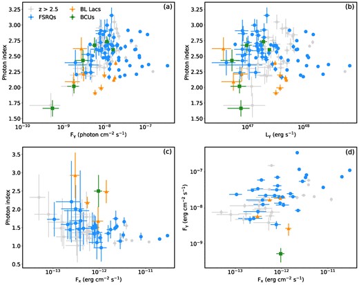
Panels (a) and (b): The γ-ray flux (>100 MeV) and luminosity versus the photon index. Panel (c) The X-ray flux versus the photon index. Panel (d) The X-ray flux versus the γ-ray flux.
Fig. 2(b) presents the γ-ray luminosity Lγ versus the photon index. This contrasts with the flux, luminosity, on the other hand, accounts for the total energy emitted by the source per unit time, so showing the intrinsic power of the sources. The luminosity of the sources under consideration spans from (3.67 ± 1.37) × 1046 erg s−1 to (6.62 ± 0.05) × 1048 erg s−1, with the lowest estimated for SDSS J105707.47+551032.2 and the highest for 4C +01.02. Notably, the luminosity of 4C +01.02 also exceeds that of B3 1343 + 451, which is the most luminous in the sample of sources with a redshift beyond 2.5. The range of luminosities for the new sample is slightly shifted towards a higher luminosity range. For instance, the luminosities of PKS 0226–559 (2.21 × 1048 erg s−1), PKS 0601–70 (1.12 × 1048 erg s−1), PKS 2149–306 (1.09 × 1048 erg s−1), S3 0458–02 (2.76 × 1048 erg s−1), 4C + 71.07 (1.48 × 1048 erg s−1), S4 0917 + 44 (1.80 × 1048 erg s−1), PKS 0446 + 11 (1.21 × 1048 erg s−1), PKS 1329–049 (1.16 × 1048 erg s−1), and 4C + 01.02 (6.62 × 1048 erg s−1) are exceeding luminosity of 1048 erg s−1, making them among the luminous blazars detected in the γ-ray band.
Fig. 2(c) shows the relationship between the X-ray photon index and the flux of the considered sources. The X-ray flux for the sources studied range from (1.06 ± 0.32) × 10−13 erg cm−2 s−1 for PMN J1344-1723 to (2.96 ± 0.02) × 10−11 erg cm−2 s−1 for 4C +71.07. The X-ray photon index is predominantly soft (less than 2.0) for the majority of the sources, suggesting that the X-ray emissions are likely dominated by the rising part of inverse Compton component. Notably, the brightest sources in the sample, such as 4C + 71.07 and PKS 2149–306, have fluxes of (2.96 ± 0.02) × 10−11 erg cm−2 s−1 and (2.01 ± 0.04) × 10−11 erg cm−2 s−1, with photon indices of 1.28 ± 0.01 and 1.19 ± 0.03, respectively. These indices indicate their X-ray spectra are particularly hard compared to the rest of the sample. Correspondingly, these two sources also show the highest X-ray luminosities, being (1.13 ± 0.11) × 1048 erg s−1 for 4C + 71.07, and (8.79 ± 1.83) × 1047 erg s−1 for PKS 2149–306.
In Fig. 2(d), a comparison of the γ-ray and X-ray fluxes for the selected sources is shown. The wide spread observed in the data suggests that there is no direct or obvious correlation between the γ-ray and X-ray fluxes when considering time-averaged measurements. It should be noted, however, that these are average values and that during shorter time-scale events, such as flares, a correlation may appear. Interestingly, the two bright in the X-ray band sources, 4C + 71.07 and PKS 2149–306, also have notably high γ-ray fluxes of (1.11 ± 0.02) × 10−7 photon cm−2 s−1 and (7.30 ± 0.20) × 10−8 photon cm−2 s−1, respectively. Conversely, the γ-ray bright source 4C + 01.02, has only a moderate X-ray flux of (2.18 ± 0.11) × 10−12 erg cm−2 s−1, indicating that a high γ-ray flux does not necessarily imply a correspondingly high X-ray flux. This discrepancy shows the complexity of the emission mechanisms and the potential influence of other factors such as beaming, the environment of the source, or the presence of different emission processes at different wavelengths.
The NuSTAR analysis results are presented in Table 2, where for each source the observation sequence, observation time, and flux in the 3–10 keV and 10–30 keV ranges, along with the photon index are provided. Three NuSTAR observations (60160099002 for S5 0212+73, 60 002 045 002 for 4C + 71.07, and 60 367 002 002 for PKS 0227–369) were relatively short (on the order of a few hundred seconds), and hence no spectral analysis was conducted. In the 3–10 keV range, the highest flux of (2.02 ± 0.01) × 10−11 erg cm−2 s−1 was observed for 4C + 71.07 on MJD 56675.22, while the lowest flux of (1.95 ± 0.27) × 10−13 erg cm−2 s−1 was observed for 87GB 080551.6+535010. The photon index for all considered sources is hard, ranging from 1.09 to 1.67, suggesting that the hard X-ray component corresponds to the rising part of the inverse Compton component. The variability of the 3–10 keV and 10–30 keV fluxes could only be investigated for 4C + 71.07 and PKS 2149–306, as multiple observations in different periods are available; however, the flux remained relatively stable.
NuSTAR analysis results.
| Source | Sequence ID | MJD | log F3–10 | log F10–30 | Photon index |
|---|---|---|---|---|---|
| 4C + 71.07 | 60 002 045 004 | 56675.22 | −10.70 ± 0.003 | −10.55 ± 0.005 | 1.63 ± 0.01 |
| 4C + 71.07 | 60 002 045 002 | 56641.65 | −10.88 ± 0.004 | −10.75 ± 0.007 | 1.67 ± 0.02 |
| PKS 2149–306 | 60 001 099 002 | 56643.22 | −10.71 ± 0.003 | −10.43 ± 0.003 | 1.35 ± 0.01 |
| PKS 2149–306 | 60 001 099 004 | 56765.64 | −10.79 ± 0.003 | −10.55 ± 0.004 | 1.45 ± 0.01 |
| S3 0458–02 | 60 367 003 001 | 58234.31 | −11.65 ± 0.014 | −11.51 ± 0.020 | 1.64 ± 0.08 |
| 87GB 080551.6 + 535010 | 80 001 004 002 | 56785.45 | −12.71 ± 0.061 | −12.30 ± 0.087 | 1.09 ± 0.28 |
| PKS 0446 + 11 | 60 101 078 002 | 57358.10 | −12.53 ± 0.059 | −12.37 ± 0.088 | 1.60 ± 0.29 |
| TXS 0322 + 222 | 60 101 079 002 | 57334.11 | −11.88 ± 0.017 | −11.54 ± 0.027 | 1.24 ± 0.09 |
| PKS 0528 + 134 | 60 160 238 002 | 58509.08 | −12.09 ± 0.034 | −11.94 ± 0.040 | 1.61 ± 0.16 |
| PKS 0227–369 | 60 367 002 002 | 57975.49 | −12.56 ± 0.055 | −12.27 ± 0.077 | 1.34 ± 0.29 |
| PKS 1329–049 | 60 160 541 002 | 57902.35 | −12.27 ± 0.043 | −12.03 ± 0.050 | 1.44 ± 0.19 |
| S5 0212 + 73 | 60 160 099 002 | 57442.46 | −11.24 ± 0.006 | −11.03 ± 0.009 | 1.52 ± 0.03 |
The source name, NuSTAR sequence ID, observation time in MJD, the logarithm of the 3–10 keV (log F3–10) and 10–30 keV (log F10–30) bands flux, and the photon index for each observation are given.
4.1 γ-ray variability
The use of adaptive binning methods for computing light curves allowed detailed investigation of the γ-ray flux variation of considered sources. Flux variations, characterized by several times increases from average levels, have been observed in 31 sources. The most variable sources in the γ-ray band, where multiple flaring activities have been observed, are PKS 0226–559, PKS 2149–306, S3 0458–02, 4C+71.07, S4 0917+44, PKS 1329–049, and 4C + 01.02. For example, the adaptively binned γ-ray light curve of PKS 0226–559, the most distant source in our sample at a redshift z = 2.464 showing variability, computed for energies above 239.66 MeV, is displayed in Fig. 3(a). From the start of Fermi-LAT observations until MJD 55 504 (2010 November 4), the γ-ray emission of this source was in a low state being (4.89 ± 0.71) × 10−9 photon cm−2 s−1. Subsequent periods of flaring activity occurred between MJD 55504.30–55584.50, 56153.18–57472.15, and MJD 58084.93–58664.52. During its most active state, between MJD 58084.93 and 58664.52, the maximum flux was (3.99 ± 0.67) × 10−7 photon cm−2 s−1 observed on MJD 58507.69. Also, the luminosity of the source significantly increased during these flaring periods. While the long-term averaged luminosity was (1.76 ± 0.04) × 1048 erg s−1, the luminosity during flares exceeded 1049 erg s−1. For example, the source luminosity was >1049 erg s−1 42 times, with the peak luminosity of (5.33 ± 0.92) × 1049 erg s−1 observed on MJD 58167.46.

The γ-ray light curve of the sources considered in this study, which show a high amplitude γ-ray flux increase during the flares. The left axis shows the variation of flux over time, while the right axis displays the luminosity.
Among the flaring sources, significant increases in γ-ray emission have been observed for PKS 2149–306, 4C+71.07, PKS 1329–049, and 4C + 01.02. For example, the time-averaged γ-ray flux of PKS 2149–306 (z = 2.345) is (2.01 ± 0.47) × 10−7 photon cm−2 s−1, but there was a notable period of elevated γ-ray emission between MJD 56288.92 and 56444.75 (Fig. 3b). During this interval, the flux above 144.85 MeV exceeded 10−6 photon cm−2 s−1 on eight time intervals. The peak flux during this period was (1.68 ± 0.33) × 10−6 photon cm−2 s−1 observed on MJD 56302.61. Additionally, the source exhibited another active γ-ray emission state between MJD 55554.39 and 55650.67. In this period, the γ-ray flux consistently exceeded 10−7 photon cm−2 s−1, with a maximum of (7.08 ± 1.22) × 10−7 photon cm−2 s−1 observed on MJD 55613.98. During multiple flaring periods of 4C + 71.07 (Fig. 3d), which is at a redshift of z = 2.218, the γ-ray emission notably exceeded its time-averaged flux of (1.06 ± 0.01) × 10−7 photon cm−2 s−1. Specifically, in three distinct flaring periods – MJD 55862.01–55932.97, MJD 57227–57245.79, and MJD 57296.92–57338.47 – the flux above 138.16 MeV exceeded 10−6 photon cm−2 s−1. The peak flux during these flaring events was at (8.02 ± 1.40) × 10−6 photon cm−2 s−1, and was observed on MJD 57335.21. The γ-ray emission of PKS 1329–049, with a redshift of z = 2.15, is predominantly in its average emission state, as depicted in Fig. 3(f). However, it exhibited an elevated emission state during the period from MJD 55442.09 to 55507.87 when the peak flux reached (2.71 ± 0.52) × 10−6 photon cm−2 s−1 observed on MJD 55445.32. In contrast, 4C + 01.02, with a redshift of z = 2.099, experiences alternating periods of flaring activity, with the most intense γ-ray flares observed after MJD 57000. The source entered an active γ-ray emission state starting from MJD 59615.91, when the peak γ-ray flux, measured above 171.79 MeV, reached (2.92 ± 0.50) × 10−6 photon cm−2 s−1 on MJD 59663.19. The other two sources, depicted in Fig. 3(c) and (e), also exhibit multiple flaring periods but with only modest increases in their γ-ray flux. Specifically, the peak γ-ray flux of S3 0458–02, measured above 202.55 MeV, was (8.32 ± 1.41) × 10−7 photon cm−2 s−1 observed on MJD 57258.92. Similarly, for S4 0917 + 44, it was (4.27 ± 0.75) × 10−7 photon cm−2 s−1 observed on MJD 57946.70.
Especially profound is the luminosity increase in 4C+71.07, PKS 1329–049, and 4C + 01.02 (see Fig. 3). For 4C + 71.07, during the flaring periods in MJD 57227–57245.79 and MJD 57296.92–57338.47, the source luminosity exceeded 1050 erg s−1 11 times. The highest luminosity of (2.03 ± 0.36) × 1050 erg s−1 was observed on MJD 57335.21. PKS 1329–049 was in an extreme bright state on MJD 55445.23 and MJD 55468.18, with luminosities of (1.07 ± 0.21) × 1050 erg s−1 and (1.39 ± 0.26) × 1050 erg s−1, respectively. Similarly, 4C + 01.02 was in an extreme bright state between MJD 59662.03–59663.55, during which in 6 consecutive bins the flux exceeded 1050 erg s−1, with the highest flux of (2.08 ± 0.48) × 1050 erg s−1 observed on MJD 59662.62. Because of such elevated luminosity, 4C+71.07, PKS 1329–049, and 4C + 01.02 rank among the sources with the highest luminosity in the γ-ray band.
In Fig. 4, the γ-ray light curves for 4C+13.14, 87GB 080551.6+535010, B2 1436+37B, PKS 0227–369, PKS 0528+134, PKS 0446+11, PKS 0601–70, S5 1053+70, and TXS 0322 + 222 are presented. For the majority of the time, the emission from these objects remains in a low to average state. However, during certain flaring periods, their γ-ray emission shows modest increases. These sources are typically weak, with γ-ray fluxes generally on the order of 10−8 photon cm−2 s−1, but there are instances when the flux exceeds 10−7 photon cm−2 s−1. For example, during an elevated γ-ray emission state, the peak flux of S5 1053 + 70 above 179.20 MeV was (1.42 ± 0.24) × 10−7 photon cm−2 s−1 observed on MJD 57684.01. Similarly, for PKS 0601–70, the highest γ-ray flux reached (1.64 ± 0.30) × 10−7 photon cm−2 s−1 on MJD 55136.37. For PKS 0446 + 11, the peak γ-ray flux was (1.77 ± 0.34) × 10−7 photon cm−2 s−1 observed on MJD 55304.46, and so on.
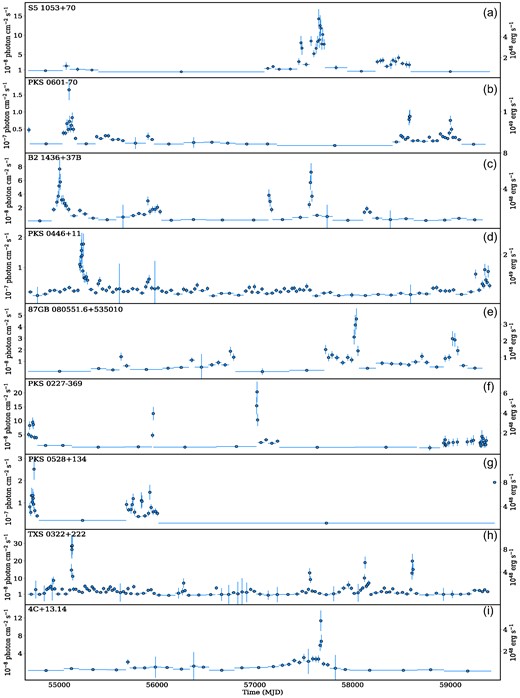
The γ-ray light curve of the sources analysed in this study, which show a modest amplitude γ-ray flux increase during the flares. The left and right axes are the same as in Fig. 3.
4.2 X-ray variability
In the considered source sample, some of the sources were observed multiple times by the Swift telescope, permitting investigation of the temporal variability of X-ray flux across different years. Among the sources considered, variability in X-ray flux was observed in 4C +71.07, PKS 0226–559, PKS 1329–049, PKS 2149–306, S3 0458–02, and S4 0917+44. For PKS 0226–559 and S4 0917 + 44, a limited number of observations were available but the ratio between the maximum and minimum fluxes is approximately 3–4, indicating temporal flux variability.
The X-ray flux variations for 4C + 71.07 (blue) and PKS 2149–306 (green) are shown in the upper panel of Fig. 5. For 4C + 71.07, the lowest observed X-ray flux was (1.00 ± 0.12) × 10−11 erg cm−2 s−1 on MJD 55247.68, while the highest was (5.63 ± 1.02) × 10−11 erg cm−2 s−1 on MJD 56832.97. Elevated X-ray emission states for this source were observed around MJD 56 000 and MJD 57000, during which most of the X-ray observations were performed. Conversely, PKS 2149–306 exhibited lower amplitude flux changes, with its highest X-ray flux being (2.92 ± 0.58) × 10−11 erg cm−2 s−1, observed on MJD 56643.02. The lower panel of Fig. 5 shows the X-ray flux variations for PKS 1329–048 (red) and S3 0458–02 (blue). Initially, the X-ray emission for S3 0458–02 was on the order of ∼10−12 erg cm−2 s−1, but it increased to approximately ∼5 × 10⁻¹² erg cm−2 s−1 around MJD 56200. For PKS 1329–048, the observed highest X-ray flux was (4.28 ± 0.68) × 10−12 erg cm−2 s−1 on MJD 55390.19, whereas it decreased to (8.99 ± 4.03) × 10−13 erg cm−2 s−1 on MJD 57902.45.
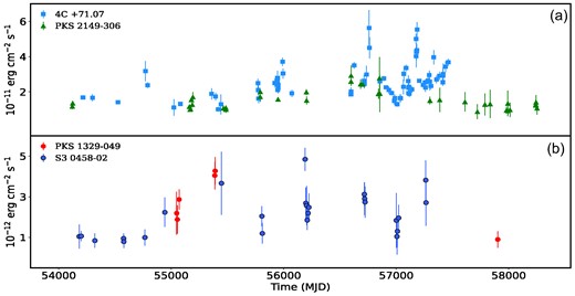
The X-ray light curve of 4C + 71.07, PKS 2149–306, PKS 1329–049, and S3 0458–02, each with multiple X-ray observations, exhibits noticeable variability.
4.3 Variability in optical/UV bands
The observations from the Swift UVOT of selected sources allows to study the flux variability within the optical/UV bands. Investigating variability is challenging when the number of observations is limited, as changes in flux up to a factor of 2 can be observed across different filters; however, this does not provide a comprehensive understanding of the flux changes in time. Notably, clear flux variability is evident in the emissions from 4C+01.02, PKS 0226–559, and PKS 2149–306. For 4C + 01.02, the initial flux measurements in the V, B, and U filters are approximately |$10^{-12} \, \text{erg} \, \text{cm}^{-2} \, \text{s}^{-1}$|, and approximately |$2 \times 10^{-13} \, \text{erg} \, \text{cm}^{-2} \, \text{s}^{-1}$| in the W1, W2, and M2 filters. After MJD 56500, the source exhibits increased flux across all filters during several observations. The highest observed flux in the B filter was |$(3.91 \pm 0.33) \times 10^{-12} \, \text{erg} \, \text{cm}^{-2} \, \text{s}^{-1}$| on MJD 57363.45. For PKS 0226–559, the mean flux is |$\sim 5 \times 10^{-13} \, \text{erg} \, \text{cm}^{-2} \, \text{s}^{-1}$|, but the flux in V filter increased up to |$(3.1-0.46) \times 10^{-12} \, \text{erg} \, \text{cm}^{-2} \, \text{s}^{-1}$| during the flare on MJD 58161.21. The UV emission from PKS 2149–306, in the W1, W2, and M2 filters, remains relatively stable across various observations, whereas the optical emission (V, B, and U) shows variability. Specifically, on MJD 53717.92, MJD 54980.86, and MJD 58586.29, the flux increased to approximately |$3 \times 10^{-12} \, \text{erg} \, \text{cm}^{-2} \, \text{s}^{-1}$|, with the lowest observed flux being around |$10^{-13} \, \text{erg} \, \text{cm}^{-2} \, \text{s}^{-1}$|.
5 MODELING OF MULTIWAVELENGTH SEDS
The data analysed in this study, combined with those collected from the archives, enabled to construct the SEDs for the selected sources from the radio to the HE γ-ray bands. The multiwavelength SEDs are presented in Fig. 6 where the data analysed in this work are highlighted in different colors (see the legend), while archival data retrieved using the VOU-Blazar tool are depicted in grey. All the SEDs exhibit the traditional double-humped structure with a clear Compton dominance (i.e. the Compton peak luminosity is significantly higher than the synchrotron peak luminosity).


The broad-band SED modeling results for the sources under consideration. The data analysed from Swift UVOT, XRT, NuSTAR, and Fermi-LAT observation are depicted in cyan, blue, orange, and red, respectively, while archival data are shown in grey. The blue line represents the combined contribution of the synchrotron, disc, SSC, and EIC-BLR components. The blue shaded area indicates the region of uncertainty associated with the model.
The selected SEDs were modeled using a leptonic one-zone synchrotron and inverse Compton model. In this scenario, the emission region is assumed to be located at a distance Rdis from the central black hole and is assumed to have a spherical geometry with a radius R. This region moves along the jet with a bulk Lorentz factor Γ and is observed at a small viewing angle, resulting in the amplification of radiation by a factor of δ ≈ Γ. The emitting region is populated with non-thermal particles (electrons and positrons), whose energy distribution follows a power law with an exponential cutoff described as
where p is the spectral index of the power-law distribution for the emitting electrons, γcut is the cutoff Lorentz factor, and γmin represents the minimum energy. Here, N0 denotes the normalization constant of the electron distribution, which defines the total energy content of the electrons as given by Ue = mc2∫γN(γ)dγ.
Within the emitting region (blob), electrons lose energy through synchrotron emission under the magnetic field B, resulting in the first bump in the multiwavelength SED. The second bump is attributed to inverse Compton scattering of low-energy photons, which may originate either internally or externally to the jet. Synchrotron photons can be inverse Compton scattered to higher energies via SSC radiation (Ghisellini, Maraschi & Treves 1985; Maraschi, Ghisellini & Celotti 1992; Bloom & Marscher 1996), and the inverse Compton scattering of external photons may also contribute to the formation of the second component. Depending on the emitting region’s proximity to the central black hole, different low-energy photon fields can be inverse Compton up-scattered: photons directly from the accretion disc (Dermer, Schlickeiser & Mastichiadis 1992; Dermer & Schlickeiser 1994), photons reprocessed by the BLR (Sikora, Begelman & Rees 1994), or photons from the dusty torus (Błażejowski et al. 2000). In the current study, we assume that the emitting region is within the BLR (Rdis < R), and that accretion disc photons reprocessed by the BLR (EIC-BLR) alongside synchrotron photons are the primary targets for inverse Compton scattering. However, we note that alternative scenarios, wherein the emitting region lies significantly closer to the central black hole or outside the BLR, cannot be excluded. Constraining the location of the emitting region requires high-quality and high-resolution data at low energy bands, which is unavailable for distant blazars and falls outside the scope of this study.
During the modeling, the accretion disc luminosity (Ldisc) and the temperature (energy) of the photons were estimated by fitting the UV band’s excess emission with a blackbody component. If the thermal component could not be distinguished, an upper limit was established by ensuring that the disc’s emission does not outshine the observed non-thermal emission from the jet. With Ldisc, the radius of the BLR is calculated using the relation RBLR = 1017L45, disc (Ghisellini & Tavecchio 2015). Subsequently, the BLR is represented as a spherical shell, with an inner boundary of Rin, BLR = 0.9 × RBLR and an outer boundary of Rout, BLR = 1.2 × RBLR.
The SEDs were fitted using the publicly available jetset code (Massaro et al. 2006; Tramacere et al. 2009; Tramacere, Massaro & Taylor 2011; Tramacere 2020), which facilitates the comparison of numerical models with observed data. For the FSRQs, the synchrotron/EIC-BLR model was used, while for the BL Lacs, the synchrotron/SSC model. Only one BCU has sufficient data for the modeling, SDSS J100326.63 + 020455 which was also modeling using synchrotron/SSC-BLR modeling considering the shape of the SED. The model consists of a combined contribution from synchrotron, disc, SSC, and EIC-BLR components, which are optimized during the fitting process. The free parameters in the model are the spectral index (p), the cutoff Lorentz factor (γcut), the minimum Lorentz factor (γmin), the magnetic field (B), the Doppler factor (δ), the size of the emitting region (R), and the energy density of the electrons (Ue). Optimization is performed in two stages: initial fitting is done with the Minuit optimizer, followed by refinement using the Markov Chain Monte Carlo method. We note that R can also be constrained by variability considerations. However, due to insufficient data for all sources, variability analysis could not be conducted. Therefore, during the fitting process, R was treated as a parameter dependent on the variability time-scale (tvar) and δ, via the relation R = δctvar/(1 + z), with tvar assumed to be within a 0.1–7-d range. However, we refrain from commenting on tvar (and consequently R) as it can only be accurately determined with high-quality data. The pair-production absorption effect due to interaction with EBL photons was incorporated using the model of Franceschini, Rodighiero & Vaccari (2008).
6 RESULTS
The modeling results are shown in Fig. 6 and the results are given in Table 3. For this modeling, we selected only those sources with sufficient data, particularly those having the X-ray data, as the HE component cannot be constrained without them. There is significant amplitude variability in some sources across optical, IR, and X-ray bands (e.g. PKS 1329–049, PKS 0446+11, 4C + 01.02, etc.), which our current modeling does not adequately interpret. To accurately model these flaring periods, a careful selection of (quasi) contemporaneous data is required. However, this is beyond the scope of the current paper, whose primary aim is to estimate the time-averaged properties of the selected sources.
Broad-band SED modeling of the considered sources.
| Source | δ | p | γmin | γcut | B | LD | Le | LB | Lp |
|---|---|---|---|---|---|---|---|---|---|
| [1] | [2] | [3] | [4] | [5] | [6] | [7] | [8] | [9] | [10] |
| S5 1053 + 70 | 18.42 ± 1.42 | 2.08 ± 0.21 | 69.49 ± 7.30 | 12.50 ± 1.22 | 3.96 ± 0.42 | 1.44 | 4.40 | 0.76 | 0.39 |
| PMN J1344-1723 | 47.18 ± 1.66 | 2.10 ± 0.06 | 18.56 ± 1.83 | 35.32 ± 3.13 | 4.21 ± 0.27 | 0.84 | 2.93 | 0.08 | 0.70 |
| PKS 1915–458 | 24.53 ± 1.14 | 2.29 ± 0.22 | 65.94 ± 6.50 | 4.09 ± 0.69 | 7.62 ± 0.80 | 4.14 | 4.55 | 0.24 | 0.62 |
| PKS 0226–559 | 33.13 ± 2.03 | 1.56 ± 0.06 | 17.32 ± 2.23 | 27.07 ± 2.54 | 4.25 ± 0.33 | 7.68 | 4.37 | 0.12 | 0.45 |
| PKS 0601–70 | 24.91 ± 1.20 | 1.92 ± 0.17 | 71.10 ± 6.49 | 6.39 ± 0.59 | 5.81 ± 0.62 | 3.23 | 3.28 | 2.43 | 0.34 |
| B2 1436 + 37B | 21.06 ± 0.96 | 2.00 ± 0.21 | 95.07 ± 10.48 | 4.69 ± 0.42 | 5.07 ± 0.57 | 0.75 | 2.64 | 1.71 | 0.25 |
| 2MASS J16561677-3302127 | 17.15 ± 0.22 | 1.93 ± 0.02 | 97.22 ± 1.59 | 14.50 ± 0.29 | 9.91 ± 0.24 | 33.50 | 6.39 | 2.56 | 0.42 |
| TXS 1645 + 635 | 24.58 ± 0.94 | 1.92 ± 0.18 | 67.97 ± 8.10 | 3.87 ± 0.37 | 7.46 ± 0.70 | 1.28 | 1.70 | 2.40 | 0.21 |
| PKS B1149-084 | 25.62 ± 0.93 | 1.92 ± 0.19 | 64.32 ± 6.41 | 4.86 ± 0.59 | 5.98 ± 0.39 | 1.98 | 1.64 | 4.50 | 0.19 |
| S5 0212 + 73 | 23.24 ± 0.65 | 2.66 ± 0.14 | 207.00 ± 9.11 | 7.63 ± 0.73 | 8.48 ± 0.38 | 9.96 | 7.23 | 0.13 | 0.39 |
| B2 0552 + 39A | 13.93 ± 0.82 | 2.12 ± 0.07 | 105.80 ± 7.80 | 27.18 ± 2.45 | 6.91 ± 0.77 | 39.70 | 5.60 | 0.43 | 0.34 |
| PKS 2149–306 | 25.83 ± 0.83 | 1.82 ± 0.04 | 83.20 ± 1.31 | 3.02 ± 0.12 | 5.14 ± 0.06 | 12.50 | 29.40 | 0.04 | 3.16 |
| PKS 1430–178 | 26.31 ± 1.22 | 2.25 ± 0.17 | 43.81 ± 5.82 | 4.17 ± 0.62 | 9.80 ± 0.83 | 6.21 | 5.32 | 0.20 | 1.00 |
| S3 0458–02 | 33.82 ± 1.37 | 2.21 ± 0.11 | 55.51 ± 7.02 | 7.16 ± 0.75 | 7.21 ± 0.59 | 6.08 | 6.60 | 1.09 | 0.93 |
| PMN J0157-4614 | 22.59 ± 1.43 | 1.94 ± 0.21 | 133.10 ± 21.74 | 4.26 ± 0.68 | 6.59 ± 0.63 | 0.69 | 0.72 | 2.63 | 0.05 |
| PKS 0420 + 022 | 26.55 ± 1.18 | 2.78 ± 0.14 | 48.92 ± 4.10 | 8.32 ± 0.95 | 8.01 ± 0.55 | 3.55 | 2.31 | 1.54 | 0.45 |
| PKS 2245–328 | 24.98 ± 1.46 | 1.94 ± 0.23 | 47.52 ± 6.02 | 4.15 ± 0.51 | 8.18 ± 0.74 | 3.06 | 2.47 | 1.86 | 0.40 |
| PKS B2224 + 006 | 21.38 ± 1.01 | 1.79 ± 0.20 | 29.27 ± 4.49 | 3.13 ± 0.38 | 8.02 ± 0.87 | 0.25 | 2.78 | 1.33 | 0.59 |
| PKS 2244–37 | 26.04 ± 1.94 | 1.99 ± 0.25 | 63.82 ± 7.72 | 5.28 ± 0.96 | 10.89 ± 1.30 | 4.46 | 1.59 | 0.03 | 0.19 |
| B2 0242 + 23 | 26.05 ± 1.26 | 2.10 ± 0.18 | 34.78 ± 4.12 | 4.95 ± 0.69 | 6.21 ± 0.48 | 1.93 | 3.08 | 0.69 | 0.62 |
| 4C + 71.07 | 32.34 ± 1.30 | 2.24 ± 0.16 | 43.72 ± 3.72 | 4.38 ± 0.40 | 9.94 ± 0.52 | 23.20 | 22.70 | 0.14 | 4.23 |
| PKS 2022 + 031 | 24.37 ± 1.31 | 2.18 ± 0.17 | 32.99 ± 3.38 | 11.10 ± 1.17 | 7.10 ± 0.84 | 0.12 | 2.32 | 0.96 | 0.45 |
| MG2 J153938 + 2744 | 19.46 ± 0.80 | 2.12 ± 0.13 | 51.00 ± 3.55 | 8.96 ± 0.96 | 8.28 ± 0.52 | 0.30 | 1.50 | 8.67 | 0.20 |
| S4 0917 + 44 | 27.14 ± 0.81 | 2.42 ± 0.11 | 69.94 ± 6.35 | 8.84 ± 0.67 | 5.32 ± 0.26 | 3.83 | 7.48 | 1.27 | 0.91 |
| PMN J2135-5006 | 5.45 ± 0.21 | 2.85 ± 0.06 | 158.70 ± 14.13 | 355.10 ± 48.94 | 1.30 ± 0.10 | 0.66 | 3.23 | 2.85 | 0.18 |
| OX 131 | 21.83 ± 0.77 | 1.60 ± 0.12 | 109.00 ± 10.71 | 13.76 ± 0.93 | 1.76 ± 0.10 | 0.41 | 4.30 | 0.04 | 0.21 |
| PMN J1959-4246 | 20.98 ± 0.84 | 2.02 ± 0.17 | 57.41 ± 4.50 | 5.07 ± 0.63 | 7.88 ± 0.71 | 0.17 | 2.54 | 1.13 | 0.34 |
| PKS 0446 + 11 | 23.19 ± 1.12 | 1.98 ± 0.17 | 16.67 ± 2.26 | 5.53 ± 0.73 | 5.34 ± 0.46 | 0.16 | 4.36 | 8.05 | 1.42 |
| PKS 1329–049 | 22.29 ± 0.87 | 2.30 ± 0.16 | 69.16 ± 8.12 | 12.00 ± 1.99 | 3.62 ± 0.34 | 6.52 | 8.00 | 0.43 | 0.87 |
| PMN J0134-3843 | 24.71 ± 0.98 | 2.54 ± 0.19 | 86.57 ± 8.43 | 4.61 ± 0.61 | 15.17 ± 0.90 | 9.01 | 1.59 | 1.40 | 0.19 |
| 87GB 080551.6 + 535010 | 26.16 ± 1.11 | 1.90 ± 0.20 | 59.01 ± 5.16 | 3.34 ± 0.34 | 4.58 ± 0.40 | 3.78 | 3.21 | 0.46 | 0.46 |
| PKS B1043-291 | 26.98 ± 1.61 | 2.50 ± 0.20 | 56.45 ± 4.78 | 10.30 ± 1.28 | 9.58 ± 1.15 | 1.89 | 1.80 | 0.88 | 0.25 |
| OM 127 | 22.03 ± 1.16 | 2.59 ± 0.14 | 49.91 ± 5.54 | 18.73 ± 3.19 | 7.31 ± 0.66 | 2.48 | 2.56 | 1.90 | 0.42 |
| PKS 0227–369 | 20.02 ± 0.68 | 2.83 ± 0.09 | 81.14 ± 8.13 | 25.89 ± 2.97 | 5.32 ± 0.50 | 2.52 | 3.59 | 1.22 | 0.41 |
| OF 200 | 15.55 ± 0.59 | 2.13 ± 0.11 | 38.66 ± 1.92 | 11.03 ± 0.68 | 5.45 ± 0.24 | 1.22 | 2.14 | 0.88 | 0.35 |
| B3 0803 + 452 | 19.64 ± 0.94 | 2.28 ± 0.25 | 44.72 ± 5.38 | 3.17 ± 0.43 | 8.56 ± 0.77 | 1.35 | 2.11 | 3.03 | 0.42 |
| 4C + 01.02 | 26.29 ± 0.98 | 1.88 ± 0.13 | 28.05 ± 2.99 | 5.55 ± 0.52 | 3.04 ± 0.19 | 2.08 | 9.23 | 5.25 | 1.88 |
| PKS 1348 + 007 | 24.93 ± 1.94 | 1.70 ± 0.21 | 59.32 ± 8.57 | 7.87 ± 0.81 | 2.50 ± 0.29 | 0.04 | 2.95 | 2.19 | 0.27 |
| SDSS J100326.63 + 020455.6 | 26.93 ± 0.76 | 2.03 ± 0.08 | 40.09 ± 1.28 | 7.69 ± 0.39 | 12.03 ± 0.28 | 1.12 | 1.75 | 0.13 | 0.27 |
| PKS 0528 + 134 | 15.71 ± 0.87 | 2.15 ± 0.10 | 46.04 ± 5.30 | 20.93 ± 2.60 | 3.67 ± 0.25 | 0.80 | 7.91 | 0.90 | 1.01 |
| TXS 0322 + 222 | 31.80 ± 0.99 | 2.12 ± 0.25 | 122.40 ± 11.04 | 2.38 ± 0.22 | 7.92 ± 0.58 | 4.45 | 3.51 | 0.51 | 0.32 |
| 4C + 13.14 | 20.30 ± 1.03 | 1.72 ± 0.14 | 44.37 ± 5.16 | 4.10 ± 0.43 | 8.13 ± 0.62 | 11.00 | 3.38 | 1.21 | 0.49 |
| PMN J0625-5438 | 12.52 ± 0.70 | 2.61 ± 0.23 | 200.50 ± 27.17 | 13.10 ± 2.07 | 5.12 ± 0.55 | 3.38 | 2.38 | 0.95 | 0.12 |
| OX 110 | 24.62 ± 0.87 | 2.08 ± 0.08 | 29.37 ± 2.40 | 18.94 ± 1.26 | 4.89 ± 0.23 | 0.86 | 1.06 | 0.29 | 0.19 |
| PKS 0549–575 | 27.49 ± 2.14 | 1.86 ± 0.21 | 37.63 ± 4.32 | 4.47 ± 0.43 | 6.42 ± 0.69 | 0.06 | 3.22 | 1.29 | 0.52 |
| PKS B1412-096 | 5.24 ± 0.17 | 2.32 ± 0.14 | 199.30 ± 17.68 | 13.22 ± 1.08 | 3.17 ± 0.26 | 2.17 | 2.20 | 40.60 | 0.10 |
| SDSS J145059.99 + 520111.7 | 40.41 ± 0.35 | 1.71 ± 0.01 | 1.41 ± 0.03 | 153.30 ± 1.30 | (1.08 ± 0.01) × 10−2 | − | 245.50 | 0.26 | 105.50 |
| PMN J0124-0624 | 49.66 ± 0.67 | 2.09 ± 0.01 | 2.67 ± 0.07 | 378.70 ± 10.95 | (1.91 ± 0.06) × 10−3 | − | 1126.00 | 0.22 | 1196.00 |
| SDSS J105707.47 + 551032.2 | 28.94 ± 0.43 | 2.15 ± 0.01 | 1.08 ± 0.03 | 2541.00 ± 47.98 | (1.72 ± 0.02) × 10−2 | − | 59.21 | 1.53 | 159.80 |
| 1RXS J032342.6-011131 | 29.71 ± 0.19 | 1.90 ± 0.004 | 1.84 ± 0.01 | 439.90 ± 5.40 | (3.99 ± 0.04) × 10−2 | − | 40.14 | 3.92 | 27.82 |
| NVSS J090226 + 205045 | 49.84 ± 0.33 | 1.79 ± 0.01 | 22.93 ± 0.23 | 212.60 ± 2.17 | (4.36 ± 0.04) × 10−3 | − | 514.00 | 1.14 | 38.29 |
| 87GB 105148.6 + 222705 | 29.10 ± 0.67 | 2.13 ± 0.01 | 2.37 ± 0.10 | 363.80 ± 10.50 | (7.32 ± 0.22) × 10−3 | − | 936.70 | 0.93 | 1235.00 |
| PKS 0437–454 | 44.39 ± 1.43 | 1.94 ± 0.01 | 1.34 ± 0.06 | 171.20 ± 5.92 | (1.65 ± 0.07) × 10−3 | − | 3852.00 | 0.10 | 4502.00 |
[1] Source Name. [2] Doppler factor. [3] Power-law index of emitting electrons. [4] Minimum Lorentz factor of the electrons and [5] cutoff Lorentz factor in units of 100. [6] Magnetic field, expressed in units of G. [7] Accretion disc luminosity, in units of 1046 erg s−1. [8] and [9] Power of the jet in the form of relativistic electrons (Le) and Magnetic field (LB), both in units of 1044 erg s−1. [10] Luminosity of the jet in the form of protons assuming one proton per relativistic emitting electron in units of 1045 erg s−1.
The EIC-BLR model was used to model all the SED of all FSRQs (46 sources). In Fig. 6, the sum of all components – the combined contribution of the synchrotron, disc, SSC, and EIC-BLR components – is depicted in blue. The emission at lower energy bands (up to X-rays) is dominated by the synchrotron and disc components, while at HEs, the SSC and EIC-BLR components are dominant. The modeling facilitates the estimation of parameters describing the jet (B, δ) as well as those characterizing the emitting electrons (p, γmin, and γcut). From the modeling of the SEDs of the FSRQs, the power-law index of the electrons varies within a range from p = 1.56 to p = 2.85, predominantly constrained by the SSC fit of the X-ray data. The hardest spectral indices are observed in sources lacking high-quality X-ray data. For instance, p = 1.56 ± 0.064 for PKS 0226–559, p = 1.60 ± 0.12 for OX 131, and p = 1.70 ± 0.21 for PKS 1348+007, etc. The power-law index of the electrons, inferred from the SSC fitting of BL Lacs (7 sources), is harder than that for FSRQs, ranging between 1.71 and 2.25. Relatively hard indices of 1.71 ± 0.01 and 1.79 ± 0.01 were estimated for SDSS J145059.99+520111.7 and NVSS J090226 + 205045, respectively.
For the FSRQs, the cutoff Lorentz factor (γcut) for the considered sources varies within a range from 237.6 to 3.53 × 10³, determined by the optical/UV and/or X-ray data. A high value of (3.55 ± 0.49) × 104 was estimated for PMN J2135-5006, which has sparse X-ray data and is therefore not considered in the discussions. The lowest value of 237.6 ± 21.8 was estimated for TXS 0322 + 222, as the shape of the low-energy data (below optical) and the optical/UV data impose a strong constraint on this parameter. A comparably high cutoff Lorentz factor, γcut = (3.53 ± 0.31) × 103, was estimated for PMN J1344-1723. In the modeling of BL Lacs, the cutoff Lorentz factor (γcut) is (1.53–25.41) × 104 which is larger than those typically estimated for EIC-BLR model, as the average energy of the synchrotron photons is lower than that of BLR photons. The highest cutoff Lorentz factor, γcut = (2.54 ± 0.05) × 105, was estimated for SDSS J105707.47 + 551032.2, which is due to the fact that the synchrotron emission of this source extends up to the X-ray band. The minimum Lorentz factor ranges from 1.08 to 207.0 and is given in Table 3, constrained by the requirement that the emission at radio bands does not overshoot the observed data.
For the FSRQs the estimated magnetic field ranges between 1.30 and 15.17 G. The highest value, 15.17 ± 0.90 G, was estimated for PMN J0134-3843 which is attributed to the fact that the synchrotron component of this source exhibits a comparable flux compared to its inverse Compton component. Consequently, when the external photons are boosted into the jet frame (with a δ = 24.71 for this object), their density increases. This requires the presence of lower density electrons, thereby requiring a higher magnetic field to account for the observed synchrotron emission. In contrast to the modeling of FSRQs, when considering BL Lacs, the magnetic field is found to be in the range of 0.001–0.04 G. For the FSRQs, except for the bordering cases of PKS B1412-096, PMN J2135-5006, and PMN J1344-1723, where δ of 5.24, 5.45, and 47.18 were estimated respectively, δ varies within a narrow range of 12.52–33.82. This range is typical for blazars. For PMN J1344-1723, a δ of 47.18 was estimated due to the pronounced Compton dominance observed in this object. In contrast, a lower δ of 5.24 for PKS B1412-096 was estimated because its Compton dominance is nearly 1. Meanwhile, δ = 5.45 for PMN J2135-5006 was estimated due to its relatively high cutoff Lorentz factor (γcut), which is unconstrained by the data. For the BL Lacs, larger δ in the range of 28.94–49.84 were estimated. This is because the synchrotron component of these objects peaks around 1013–1014 Hz, so a higher δ is required to explain the second peak, which is in the MeV band.
Another key parameter to assess following the modeling is the jet luminosity. The jet power, in the form of electrons and magnetic field, is computed as |$L_{e}=\pi c R_b^2 \Gamma ^2 U_{e}$| and |$L_{B}=\pi c R_b^2 \Gamma ^2 U_{B}$|, respectively. Assuming one proton per relativistic emitting electron and that protons are ‘cold’ in the comoving frame, the total jet luminosity is calculated as Ljet = Le + LB + Lp. The corresponding Le and LB luminosities are presented in Table 3. For the FSRQs, Le varies within the range from 7.24 × 1043 erg s−1 to 2.94 × 1045 erg s−1, while LB ranges from 2.72 × 1042 erg s−1 to 4.06 × 1045 erg s−1. Among the considered sources, 33 exhibit an Le/LB ratio in the range of 0.1 to 10, suggesting that the emitting region is close to equipartition. For PKS B1412-096 the ratio Le/LB = 0.05 is estimated which is because of the synchrotron component is at the same level as the inverse Compton component. Conversely, for OX 131, 4C + 71.07, and PKS 2149–306, a significantly higher ratio with Le/LB > 100 is estimated, due to the dominance of the SSC component over the synchrotron component. In the modeling of BL Lacs, Le is in the range of (0.04–3.85) × 1047 erg s−1, which is higher than the LB, ranging from (0.10–3.92) × 1043 erg s−1. The relationship between the total jet luminosity (Ljet) and redshift is illustrated in Fig. 7 upper panel, where our current source sample (FSRQs in blue and BL Lacs in orange) is compared with sources from Sahakyan et al. (2020; grey), all of which are FSRQs. Clearly, BL Lacs exhibit different properties and tend to have higher luminosities. However, discussions about the distribution of BL Lacs remain inconclusive. This is because BL Lacs are rarely identified at distances z > 2.0 but a significant fraction of BL Lacs lack robust redshift determination, suggesting that BL Lacs might indeed be present at larger redshifts. In contrast, FSRQs show a similar luminosity range to those at redshifts z > 2.5. For the FSRQs the highest luminosity of 6.51 × 1045 erg s−1 was observed for 4C + 71.07 at a redshift of z = 2.218. Upon comparing both samples, it is evident that the jet luminosity tends to increase with source distance, with two notable exceptions: PKS 1351–018 and GB 1508 + 5714, which have the highest redshifts of z = 3.72 and z = 4.31, respectively.
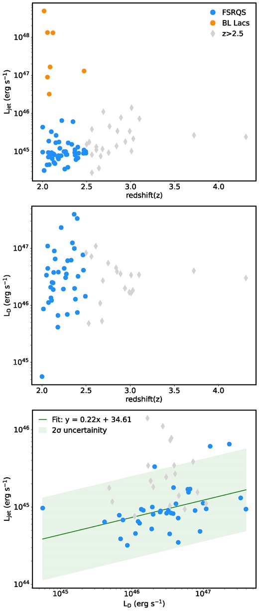
Upper panel: The dependence of the total jet luminosity (Ljet) on redshift. Middle panel: The dependence of the disc luminosity (LD) on redshift. Lower panel: The correlation between jet luminosity and disc luminosity. The sources from Sahakyan et al. (2020) are shown by diamonds.
The fit presented in Fig. 6 also enables the estimation of disc luminosity for cases where a thermal blue-bump component is observable. This excess is evident in a total of 37 sources. The disc luminosity, LD, varies from 5.60 × 1044 erg s−1 to 3.97 × 1047 erg s−1. The relationship between disc luminosity and redshift for γ-ray blazars with z > 2.0 is depicted in the middle panel of Fig. 7. High disc luminosities of 1.25 × 1047 erg s−1, 2.32 × 1047 erg s−1, 3.35 × 1047 erg s−1, and 3.97 × 1047 erg s−1 were estimated for PKS 2149–306, 4C +71.07, 2MASS J16561677-3302127, and B2 0552 + 39A, respectively. Furthermore, the relationship between disc luminosity and jet luminosity is examined in the lower panel of Fig. 7. This relationship can be described by the equation log10(Ljet) = 0.22 × log10(LD) + 34.60, represented by the green line in Fig. 7, with the 2σ uncertainty region shown in light green. Notably, sources such as PKS 2149–306 and 4C + 71.07 exhibit disc luminosities exceeding 1047 erg s−1 and jet luminosities exceeding 1045 erg s−1, highlighting their significant energetic output.
7 CONCLUSION
High redshift blazars have consistently been the subject of intense investigation due to their crucial role in understanding the connection between jet formation, accretion processes, and black hole development in the early stages of black hole formation. In this paper, we investigate the multiwavelength properties of 79 blazars with redshifts ranging from z = 2.0 to 2.5 using data accumulated by Fermi, Swift XRT/UVOT, and NuSTAR.
In the γ-ray band, the flux and photon index of the selected sources span from 5.32 × 10⁻¹⁰ to 3.40 × 10⁻⁷ photon cm−2 s−1 and between 1.66 and 3.15, respectively, illustrating the diverse characteristics of the sources under consideration. Meanwhile, the luminosity ranges from (3.67 ± 1.37) × 1046 to (6.62 ± 0.05) × 1048 erg s−1, positioning some of these sources among the brightest blazars detected in the γ-ray band. Similarly, in the 0.3–10 keV band, the weakest sources exhibit fluxes on the order of (1.06 ± 0.32) × 10−13 erg cm−2s−1, while the brighter ones reach (2.96 ± 0.02) × 10−11 erg cm−2s−1, with the majority of the sources exhibiting a soft photon index (less than 2.0). This soft photon index extends into the hard X-ray band (3–30 keV), where the index ranges from 1.09 to 1.67. The comparison of γ-ray and X-ray fluxes reveals no clear correlation in time-averaged measurements. This is exemplified by sources such as 4C +71.07 and PKS 2149–306, which are bright in both γ-ray and X-ray bands, and 4C + 01.02, which, despite its high γ-ray flux, exhibits only a moderate X-ray flux.
Using the adaptive binning methods for light curve, we found flux variations in 31 sources, with the most pronounced variability in 4C+01.02, 4C+71.07, PKS 0226–559, PKS 1329–049, PKS 2149–306, S3 0458–02, and S4 0917+44. The sources like PKS 2149–306, 4C+71.07, PKS 1329–049 and 4C + 01.02 showed significant increases in γ-ray emission, with peak fluxes occasionally exceeding 10−6 photon cm−2 s−1 while for the other sources show more modest increases in γ-ray flux: the γ-ray fluxes exceed 10−7 photon cm−2 s−1 during flaring periods. Noticeably, the γ-ray luminosity of 4C+71.07, PKS 1329–049, and 4C + 01.02 occasionally was above 1050 erg s−1, putting them among the most luminous sources in the γ-ray band.
In addition to γ-ray variability, our analysis extended to X-ray and optical/UV bands. Despite the limited data, X-ray flux variability was evident for 4C +71.07, PKS 0226–559, PKS 1329–049, PKS 2149–306, S3 0458–02 and S4 0917+44, while in optical/UV band clear flux variation is found for 4C + 01.02, PKS 0226–559, and PKS 2149–306.
In this study, we employed a leptonic one-zone synchrotron and inverse Compton model, considering both internal and external photons, to interpret the multiwavelength SEDs of selected FSRQs and BL Lacs. The range of parameters estimated from the modeling provides a general view of the sources’ emissions in an average state. The power-law index of the electrons, indicative of particle acceleration mechanisms, varied from 1.56 to 2.85. For FSRQs the highest energy emissions, as characterized by the cutoff Lorentz factor, varied broadly from 237.6 to 3.53 × 10³, reflecting the diverse characteristics of the sources studied. The total jet luminosity varied within a relatively narrow range from 3.20 × 1044 to 6.51 × 1045 erg s−1. The disc luminosity, estimated for sources with discernible thermal components in their SEDs, provided insights into the accretion processes. These disc luminosities, ranging dramatically from 4.15 × 1044 to 3.97 × 1047 erg s−1, highlighted the varying scales of accretion efficiency and energy conversion in these sources.
In summary, this comprehensive study of 79 high-redshift blazars illuminates the intricate dynamics and energetic processes at play in these distant and powerful objects. Our findings, encompassing a broad spectrum of multiwavelength observations, highlight the diverse characteristics and behaviors of blazars, underscoring their value in probing the physics of jet formation and accretion processes, and black hole development in the early Universe. The observed variations in flux and luminosity across different bands provide key insights into the particle acceleration and emission mechanisms. Future investigations, when a larger number of distant blazars are known, will allow a more systematic and statistical comparison of their emission properties, thereby unveiling the complexities of these energetic sources and providing a window into the HE universe and its evolution over cosmic time.
ACKNOWLEDGEMENTS
We acknowledge the use of analysis tools and services from the Markarian Multiwavelength Data Center (https://mmdc.am), the Astrophysics Science Archive Research Center (HEASARC) platforms, as well as data from the Fermi-LAT, Swift, and NuSTAR telescopes. This work was support by the Higher Education and Science Committee of the Republic of Armenia, in the frames of the research project No. 21T-1C260.
DATA AVAILABILITY
The data underlying this article will be shared on reasonable request to the corresponding author.
