


ABSTRACT
The galaxy–galaxy lensing technique allows us to measure the subhalo mass of satellite galaxies, studying their mass-loss and evolution within galaxy clusters and providing direct observational validation for theories of galaxy formation. In this study, we use the weak gravitational lensing observations from Dark Energy Spectroscopic Instrument (DESI) Legacy Imaging Surveys DR8, in combination with the redMaPPer galaxy cluster catalogue from Sloan Digital Sky Survey (SDSS) DR8 to accurately measure the dark matter halo mass of satellite galaxies. We confirm a significant increase in the stellar-to-halo mass ratio of satellite galaxies with their halo-centric radius, indicating clear evidence of mass-loss due to tidal stripping. Additionally, we find that this mass-loss is strongly dependent on the mass of the satellite galaxies, with satellite galaxies above |$10^{11}~{{\rm M}_{\odot }}\, h^{-1}$| experiencing more pronounced mass-loss compared to lower mass satellites, reaching 86 per cent at projected halo-centric radius 0.5R200c. The average mass-loss rate, when not considering halo-centric radius, displays a U-shaped variation with stellar mass, with galaxies of approximately |$4\times 10^{10}~{{\rm M}_{\odot }}\, h^{-1}$| exhibiting the least mass-loss, around 60 per cent. We compare our results with state-of-the-art hydrodynamical numerical simulations and find that the satellite galaxy stellar-to-halo mass ratio in the outskirts of galaxy clusters is higher compared to the predictions of the Illustris-TNG project about factor 5. Furthermore, the Illustris-TNG project’s numerical simulations did not predict the observed dependence of satellite galaxy mass-loss rate on satellite galaxy mass.
1 INTRODUCTION
In the framework of modern cold dark matter cosmology, dark matter haloes form hierarchically. In the early universe, the first to form are small dark matter haloes, which grow into larger ones by merging and accreting matter (Frenk & White 2012). Gas collapses and condenses in the centres of dark matter haloes, igniting stars and forming galaxies. Galaxies also evolve together with dark matter haloes. When a small halo falls into a larger one, it experiences dynamical friction, tidal stripping, and tidal heating effects, gradually losing mass and eventually disintegrating (e.g. Gao et al. 2004, 2012; Springel et al. 2008; Xie & Gao 2015; Han et al. 2016; Niemiec et al. 2019, 2022). In this process, galaxies transform into satellite galaxies within larger haloes, and their gas is removed through tidal stripping and ram pressure stripping, leading to the quenching of star formation (e.g. Wang et al. 2007; Guo et al. 2011; Wetzel et al. 2014). Investigating the co-evolution of satellite galaxies and subhaloes in observations will provide key clues to the picture of galaxy formation.
Measuring the masses of subhaloes hosting satellite galaxies is a challenge, not only because dark matter does not emit light and can only be detected through its gravitational effects, such as gravitational lensing, but also because the subhaloes hosting satellite galaxies have very small masses. In observations, the technique of strong gravitational lensing is employed to study the individual subhaloes of lensing galaxies. These subhaloes, distributed on the scale of the Einstein ring, can perturb the light path and manifest as flux-ratio anomalies (Mao & Schneider 1998; Metcalf & Madau 2001; Nierenberg et al. 2014) or flux perturbations in the strong lensing images (e.g. Koopmans 2005; Vegetti & Koopmans 2009; Vegetti et al. 2010, 2012; Li et al. 2016b, 2017; He et al. 2022, 2023; Nightingale et al. 2022). Such observations primarily involve dark matter haloes with masses less than 1010 M⊙. In the case of strong lensing by galaxy clusters, the dark matter haloes of massive satellite galaxies can induce image displacements and variations in the brightness of extended arcs (e.g. Kneib et al. 1996; Natarajan et al. 2009; Kneib & Natarajan 2011). Although strong gravitational lensing can provide insights into the mass of individual subhaloes, these events are rare and typically concentrated in the central regions of galaxies or galaxy clusters. Consequently, obtaining comprehensive measurements of the mass and evolution of satellite galaxy subhaloes in galaxy groups and clusters remains challenging.
An alternative effective method for measuring the subhaloes of satellite galaxies in galaxy groups and clusters is through the technique of galaxy–galaxy gravitational lensing, which measures tangential shear around a sample of selected galaxies (e.g. Brainerd, Blandford & Smail 1996; Hoekstra et al. 2003; Mandelbaum et al. 2005, 2006; Mandelbaum, Seljak & Hirata 2008; Cacciato et al. 2009; Li et al. 2009; Fu & Fan 2014). The measurement can probe the distribution of dark matter around the selected galaxy sample, thus helping to explore the connection between visible and invisible matter. In the context of galaxy–galaxy lensing, satellite galaxies can be selected from optically confirmed galaxy clusters or galaxy groups. By studying the gravitational lensing signal around these satellite galaxies, researchers can investigate the mass distribution of subhaloes, shedding light on the connection between the satellite galaxies and the subhaloes in which they reside (e.g. Yang et al. 2006; Li et al. 2013).
Li et al. (2014) utilized data from the CFHT-STRIPE82 survey (CS82; Comparat et al. 2013) and combined it with the SDSS galaxy group catalogue constructed by Yang et al. (2007). They provided the first measurement of the galaxy–galaxy lensing signals for satellite galaxies. In Li et al. (2016a), they further measured the lensing signals for satellite galaxies in the redMaPPer galaxy cluster catalogue and found that the subhalo masses of satellite galaxies increase with their halo-centric radius, providing clear evidence of satellite galaxy mass-loss. They also split the satellite galaxies into two mass bins and show that the satellite galaxies with larger stellar mass retain large dark matter subhalo. Sifón et al. (2015) measured the satellite galaxy lensing signals in the Galaxy And Mass Assembly survey (GAMA; Driver et al. 2011) and found that while satellite galaxies exhibit significant mass-loss compared to field galaxies, their stellar-to-halo mass ratio (SHMR) does not show a clear variation with halo-centric radius. Sifón et al. (2018) measured satellite galaxy–galaxy lensing with Multi-Epoch Nearby Cluster Survey (Sand et al. 2012) and found a discontinuity trend of SHMR as a function of halo-centric radius. van Uitert et al. (2016) measured the galaxy–galaxy lensing signals in the GAMA survey and found no significant difference in the mass-to-light ratio between satellite galaxies and field galaxies. Niemiec et al. (2017) combined data from the CFHTLens survey, CS82 survey, and DES-SV survey to measure the gravitational lensing signals of satellite galaxies in the redMaPPer galaxy clusters. They confirmed that the mass-to-light ratio of satellite galaxies evolves with a halo-centric radius and calculated an average mass-loss rate of approximately 70–80 per cent compared to field galaxies. Finally, Dvornik et al. (2020) measure the satellite galaxy–galaxy lensing for both central and satellite galaxies in the GAMA survey with shear catalogue from Kilo-Degree Survey, they confirmed that SHMR of satellite galaxies shifted towards lower halo masses by ∼20–50 per cent due to stripping mass-loss. In summary, the results from different observational data sets show some discrepancies, indicating the need for improved data to accurately determine the evolution of subhaloes hosting satellite galaxies in the environment of their host haloes.
In this project, we utilized the weak gravitational lensing measurements from the Dark Energy Spectroscopic Instrument (DESI) Legacy Imaging Surveys (DECaLs; Dey et al. 2019), covering an area of 9500 deg2. We combined these measurements with the redMaPPer galaxy cluster catalogue from the SDSS Data Release 8 (Aihara et al. 2011) survey to perform galaxy–galaxy lensing measurements of satellite galaxies. This allowed us to obtain higher signal-to-noise ratio (S/N) lensing signals for satellite galaxies, calculate their subhalo mass, and derive their mass-loss rates after infall more accurately.
The structure of our paper is as follows: In Section 2, we introduce the observational data we used. In Section 3, we describe the methodology for galaxy–galaxy lensing calculations and lensing model. In Section 4, we present our measurement results and discussion. Finally, in Section 5, we provide our summary and conclusions. Throughout the paper, we adopt a flat Lambda cold dark matter cosmological model from the WMAP9 results (Hinshaw et al. 2013; i.e. Ωm = 0.2865, |$\rm \mathit{ H}_{\rm 0}=69.32\, \rm {kms^{-1}\,Mpc^{-1}}$|).
2 OBSERVATIONAL DATA
In this project, we utilize satellite galaxies from the redMaPPer galaxy cluster as lenses and galaxies from the DECaLS Data Release 8 as sources. This section provides a description of these data sets.
2.1 Lens galaxies
This study utilizes satellite galaxies in the redMaPPer cluster as gravitational lenses. The redMaPPer algorithm (redMaPPer; Rozo & Rykoff 2014a; Rykoff et al. 2014) groups red-sequence galaxies with similar redshifts and spatial concentrations based on their ugriz magnitudes and errors to identify galaxy clusters. In this work, we use version 6.3 of the redMaPPer cluster catalogue1 of SDSS Data Release 8 (DR8), which covers 10 000 deg2 of the sky, contains 26 111 galaxy clusters (Aihara et al. 2011). In the redMaPPer catalogue, each cluster is assigned a richness parameter λ based on the number of red-sequence galaxies brighter than 0.2L* at the cluster’s redshift within a scaled aperture. This parameter has been shown to be a good proxy for the galaxy cluster halo mass (Rozo & Rykoff 2014a). For this project, we select galaxy clusters with a richness λ > 20. We also require that our galaxy clusters reside within a redshift range of 0.1 < z < 0.5, where the lower bound ensures lensing efficiency and the higher bound ensures reliable richness measurements (Rozo et al. 2014b).
For each redMaPPer cluster, the potential member is assigned a probability of membership Pmem according to their photometric redshift, colour, and their cluster-centric distance. To reduce the contamination induced by fake member galaxies, we only use satellite galaxies with membership probability Pmem > 0.8 and this selection criterion can remove most contamination (Niemiec et al. 2017; Zu et al. 2017).
When calculating the lensing signal, we use the redshift of the central galaxy of each redMaPPer galaxy cluster as the redshift of the satellite galaxies, as the majority of central galaxies have spectroscopic redshifts. We make use of the stellar mass information derived by Zou et al. (2019), where the stellar mass is estimated by applying the Bayesian spectral energy distribution (SED) model fitting with the Le Phare code2 (Ilbert et al. 2009). Zou et al. (2019) adopted the default BC03 spectral models with the Chabrier (2003) initial mass function. Readers are referred to Zou et al. (2019) for more details. In this project, we select satellite galaxies within a stellar mass region of [|$10^{10}~{\rm M_{\odot }}\, h^{-1}$|, |$10^{12}~{\rm M_{\odot }}\, h^{-1}$|].
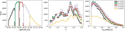
We divide the satellite galaxies into six bins according to their comoving projection cluster-centric distance Rp. The ranges of Rp bins and the number of satellite galaxy lenses in each bin are shown in Table 1. We show the distribution of stellar mass M*, redshift z, and comoving projected cluster-centric distance Rp of each bin in Fig. 1.
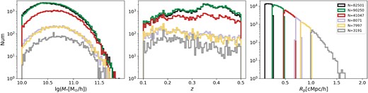
Histogram of M*, z, and Rp for the six bins listed in Table 1. The six bins are shown in sequence from left to right in the third panel. Subsamples in different panels share the same colours.
Number of lenses in each subsample. The bins are separated with the Rp value, as shown in the second column. In the following columns, the parameters of each bin are listed in sequence, the number of lenses of subsample, the average redshift, the average projection cluster-centric physical distance, the average comoving projection cluster-centric physical distance, the average stellar mass, host halo normalization α, subhalo mass, SHMR, and dark matter strip rate. All the masses are in unit of |${\rm M_{\odot }}\, h^{-1}$| and distance in Mpc h−1.
| Rp range | Num | <z> | <Rpp> | <Rp> | lg(<M*>) | α | rsub | lg(Menh) | Menh/<M*> | τstrip | |
|---|---|---|---|---|---|---|---|---|---|---|---|
| All M* | 0.1–0.25 | 825 01 | 0.33 | 0.13 | 0.17 | 10.69 | |$0.99_{-0.01}^{+0.01}$| | |$0.05_{-0.01}^{+0.01}$| | |$11.38_{-0.11}^{+0.09}$| | |$4.87_{-1.08}^{+1.15}$| | |$0.94_{-0.01}^{+0.01}$| |
| 0.25–0.47 | 902 50 | 0.33 | 0.26 | 0.35 | 10.71 | |$0.98_{-0.02}^{+0.02}$| | |$0.14_{-0.01}^{+0.01}$| | |$11.94_{-0.07}^{+0.07}$| | |$16.89_{-2.63}^{+2.94}$| | |$0.78_{-0.04}^{+0.03}$| | |
| 0.47–0.7 | 410 47 | 0.31 | 0.44 | 0.57 | 10.77 | |$0.99_{-0.04}^{+0.04}$| | |$0.25_{-0.03}^{+0.03}$| | |$12.25_{-0.1}^{+0.09}$| | |$30.27_{-5.97}^{+7.11}$| | |$0.66_{-0.08}^{+0.07}$| | |
| 0.7–0.8 | 8071 | 0.28 | 0.59 | 0.75 | 10.79 | |$1.03_{-0.04}^{+0.04}$| | |$0.3_{-0.04}^{+0.04}$| | |$12.47_{-0.14}^{+0.12}$| | |$47.58_{-12.96}^{+15.3}$| | |$0.57_{-0.14}^{+0.12}$| | |
| 0.8–1.0 | 7997 | 0.26 | 0.71 | 0.88 | 10.81 | |$0.98_{-0.05}^{+0.04}$| | |$0.38_{-0.05}^{+0.06}$| | |$12.63_{-0.12}^{+0.11}$| | |$65.51_{-15.59}^{+18.43}$| | |$0.42_{-0.16}^{+0.14}$| | |
| 1.0–2.0 | 3191 | 0.26 | 0.89 | 1.12 | 10.83 | |$1.03_{-0.09}^{+0.08}$| | |$0.47_{-0.09}^{+0.11}$| | |$12.72_{-0.2}^{+0.17}$| | |$76.78_{-28.75}^{+36.54}$| | |$0.24_{-0.36}^{+0.29}$| | |
| High M* | 0.1–0.25 | 8170 | 0.35 | 0.13 | 0.17 | 11.18 | |$0.98_{-0.05}^{+0.04}$| | |$0.09_{-0.01}^{+0.02}$| | |$12.02_{-0.15}^{+0.14}$| | |$6.87_{-2.0}^{+2.67}$| | |$0.96_{-0.01}^{+0.01}$| |
| 0.25–0.47 | 9943 | 0.35 | 0.26 | 0.35 | 11.18 | |$0.95_{-0.07}^{+0.06}$| | |$0.18_{-0.03}^{+0.04}$| | |$12.3_{-0.17}^{+0.16}$| | |$13.31_{-4.32}^{+6.04}$| | |$0.92_{-0.04}^{+0.03}$| | |
| 0.47–0.7 | 5955 | 0.34 | 0.43 | 0.57 | 11.18 | |$1.11_{-0.12}^{+0.11}$| | |$0.27_{-0.07}^{+0.08}$| | |$12.6_{-0.19}^{+0.18}$| | |$25.74_{-9.3}^{+13.21}$| | |$0.86_{-0.07}^{+0.05}$| | |
| Low M* | 0.1–0.25 | 8170 | 0.33 | 0.13 | 0.17 | 10.58 | |$0.99_{-0.01}^{+0.01}$| | |$0.05_{-0.01}^{+0.01}$| | |$11.25_{-0.15}^{+0.12}$| | |$4.74_{-1.39}^{+1.46}$| | |$0.85_{-0.05}^{+0.05}$| |
| 0.25–0.47 | 9943 | 0.33 | 0.26 | 0.35 | 10.59 | |$0.99_{-0.02}^{+0.02}$| | |$0.13_{-0.01}^{+0.01}$| | |$11.88_{-0.08}^{+0.08}$| | |$19.24_{-3.38}^{+3.79}$| | |$0.38_{-0.12}^{+0.11}$| | |
| 0.47–0.7 | 5955 | 0.3 | 0.44 | 0.56 | 10.63 | |$0.98_{-0.05}^{+0.04}$| | |$0.24_{-0.03}^{+0.04}$| | |$12.16_{-0.12}^{+0.11}$| | |$33.67_{-8.11}^{+9.81}$| | |$-0.05_{-0.31}^{+0.25}$| |
2.2 Source galaxies
The source galaxies catalogue for weak lensing analysis is extracted from data release 8 (DR8) of the DECaLs (Dey et al. 2019), and has been used in multiple scientific studies (e.g. Phriksee et al. 2020; Yao et al. 2020; Xu et al. 2021; Zu et al. 2021; Wang et al. 2023), due to its large sky coverage of approximately 9500 deg2 in grz bands.
The DECaLS DR8 data are processed by Tractor (Lang, Hogg & Schlegel 2016; Meisner, Lang & Schlegel 2017). The morphologies of sources are divided into five types, including point sources, simple galaxies (SIMP; an exponential profile with affixed 0|${_{.}^{\prime\prime}}$|45 effective radius and round profile), DeVaucouleurs (DEV; elliptical galaxies), Exponential (EXP; spiral galaxies), and Composite model (COMP; deVaucouleurs + exponential profile with the same source centre).3 Sky-subtracted images are stacked in five different ways: one stack per band, one flat SED stack of the g, r, z bands, and one red SED stack of all bands (g − r = 1 mag and r − z = 1 mag). Sources above the 6σ detection limit in any stack are kept as candidates. Galaxy ellipticities (e1, e2) are estimated by a joint fitting image of g, r, and z bands for SIMP, DEV, EXP, and COMP galaxies. The multiplicative bias (m) and additive biases (e.g. Heymans et al. 2012; Miller et al. 2013) are modelled by calibrating with the image simulation (Phriksee et al. 2020) and cross-matching with external shear measurements (Phriksee et al. 2020; Yao et al. 2020; Zu et al. 2021), including the Canada–France–Hawaii Telescope (CFHT) Stripe 82 (Moraes et al. 2014), Dark Energy Survey (Abbott et al. 2016), and Kilo-Degree Survey (Hildebrandt et al. 2017) objects.
The photo-z of each source galaxy in DECaLS DR8 shear catalogue is taken from Zou et al. (2019), where the redshift of a target galaxy is derived with its k-nearest-neighbour in the SED space whose spectroscopic redshift is known. The photo-z is derived using five photometric bands: three optical bands, g, r, and z from DECaLS DR8, and two infrared bands, W1, W2, from Wide-Field Infrared Survey Explorer. By comparing with a spectroscopic sample of 2.2 million galaxies, Zou et al. (2019) show that the final photo-z catalogue has a redshift bias of |$\Delta \overline{z}_{\rm norm}=2.4\times 10^{-4}$|, the accuracy of |$\sigma _{\Delta z_{\rm norm}}=0.017$|, and outlier rate of about 5.1 per cent.
3 METHODS
3.1 Lensing signal
The excess surface density, ΔΣ(R) is calculated as
where
|$\overline{\Sigma }(\lt R)$| is the mean density within radius R and the |$\overline{\Sigma }(R)$| is the azimuthally averaged surface density at radius R (e.g. Miralda-Escude 1991; Wilson et al. 2001; Leauthaud et al. 2010). Here, γt is the tangential shear and Σcrit is the critical surface density containing space geometry information. Here, Ds, Dl, and Dls are the angular diameter distances between the observer and the source, the observer and the lens, and the source and the lens, respectively. The c here is the constant of light velocity in the vacuum. ωn is a weight factor introduced to account for intrinsic scatter in ellipticity and shape measurement error of each source galaxy (Miller et al. 2007, 2013). The ωn we used in this work is defined as |$\omega _{\rm n}=1/(\sigma ^2_{\epsilon }+\sigma ^2_{\rm e})$|. σϵ = 0.27 is the intrinsic ellipticity dispersion derived from the whole galaxy catalogue (Giblin et al. 2021). σe is the error of the ellipticity measurement defined in Hoekstra et al. (2002). Owing to the photo-z uncertainties of the source galaxies, we remove the lens–source pairs with zs − zl < 0.1 or zs − zl < σl + σs. σl and σs are redshift errors of lens and source, respectively.
We apply the correction of multiplicative bias to the measured excess surface density as
where
where m is the multiplicative error as described in Section 2.2. In this work, we use the Super W Of Theta (swot) code4 (Coupon et al. 2011) to calculate the excess surface density.
We stack the tangential shear around satellite galaxies in six subsamples of Rp bins as listed in Table 1. For subsamples of 0.1 < Rp < 0.25, 0.25 < Rp < 0.47, and 0.47 < Rp < 0.7, we calculate galaxy–galaxy lensing in 35 linear radial bins ranging from 0.05 to 1 Mpc h−1 in comoving coordinates. For the larger Rp bins, we use 20 linear radial bins ranging from 0.05 to 1.75 Mpc h−1 in comoving coordinates.
3.2 Lensing model
The excess surface density around a satellite galaxy is composed of three components:
where the ΔΣsub is the contribution from the subhalo in which the satellite galaxy resides, ΔΣhost is the contribution from the host halo of the cluster, where Rp is the projected distance from the satellite galaxy to the centre of the host halo, and ΔΣstar is the contribution from the stellar component of the satellite galaxy. Since the contribution from the two-halo term is only significant at |$R\gt 3~{\rm Mpc}\, h^{-1}$| for clusters (Shan et al. 2017), it cannot affect the region where satellite galaxies dominate. Therefore, we have neglected the two-halo term.
Subhalo contribution
Different mass density models of subhalo were studied using gravitational lensing (Sifón et al. 2015, 2018; Li et al. 2016a; Niemiec et al. 2017). The two most commonly used models are the NFW model (Navarro, Frenk & White 1997) and the truncated-NFW (tNFW) profile (Baltz, Marshall & Oguri 2009; Oguri & Hamana 2011). In this study, we choose the NFW profile model as the subhalo mass density model.
where rs is the characteristic scale of the halo where the local logarithmic slope reaches |$\frac{{\rm d}~\ln \rho }{{\rm d}~\ln r}=-2$|. The critical density of the universe is written as
where H(z) is Hubble parameter at redshift z and the G is Newton’s constant.
CΔ = RΔ/rs is the concentration parameter, RΔ is a radius where the average density of the halo within it is Δ times of the mean matter mass density ρcritΩm(z) of the universe at redshift z, where Ωm(z) is the matter density parameter at redshift z. The enclosed mass within RΔ is |$M_{\Delta }=\frac{4\Delta \pi }{3}\rho _{\rm crit}\Omega _{\rm m}(z)R_{\Delta }$|. In this study, we choose Δ = 200. The free parameters of this model are M200m and C200m. The corresponding halo radius is R200m. In the latter part of the paper, we also use another definition of halo radius R200c, which represents the radius within which the mean density of the halo is 200 times the critical density of the universe at the redshift z the halo located. The corresponding mass and concentration are denoted as M200c and C200c, respectively.
By integrating the three-dimensional (3D) density profile along the line of sight, we can get the projected surface density ΣNFW(R) which is a function of the projection radius R,
Integrating ΣNFW(R) from 0 to R, we can get the mean surface density within R, |$\overline{\Sigma } _{\rm NFW}(\lt R)$|, as follows,
The lensing signal produced by the NFW profile is
Note that the quantity M200m and C200m of the subhalo density profile are used for mathematical convenience only, not physically meaningful for subhaloes whose outer part has been stripped in their host haloes. In this paper, we define subhalo masses, Menh as the sum of dark matter mass within the subhalo radius, rsub, at which the subhalo dark matter mass density equals to the background mass density of the cluster (Natarajan, De Lucia & Springel 2007; Sifón et al. 2018). The subhalo radius rsub is determined by measuring the mean mass density within a small sphere around the substructure and subtracting from it the mass in the same sphere after spherically averaging the entire mass distribution of the halo around the halo centre. This provides an estimate of the background density in the volume occupied by the substructure. During the computation of rsub, it is necessary to have knowledge of the three-dimensional halo-centric radius R3d. Assuming that the satellite galaxy number density distribution follows the NFW model distribution and is consistent with the distribution of dark matter particles in the host halo, then statistically, the average of the three-dimensional cluster-centric distance of the dark matter particles (satellite galaxies) projected on to the Rp radius can be expressed as follows,
where |$a=\sqrt{(3R_{\rm 200m,host})^2-R_{\rm p}^2}$| and ρ(r) is the mass density profile of host halo. The mass and concentration of the host halo mass model are shown in the following host halo model part.
Host halo model
We assume that the profile of a host halo in a galaxy cluster follows the NFW profile, the contribution from the host halo can be expressed as follows according to Yang et al. (2006).
To calculate the lensing signal for each galaxy cluster, the values of M200m and C200m of host halo are obtained through the λ−M200m relation presented by Rykoff et al. (2012),
as well as the M200m−C200m relation proposed by Xu et al. (2021) ,
where |$C_{0}=5.119^{+0.183}_{-0.185}$|, |$\gamma =0.205^{+0.010}_{-0.010}$|, |${\rm lg(}M_{0}{\rm)}=14.083^{+0.130}_{-0.133}$| when 0.08 < z < 0.35 and |$C_{0}=4.875_{-0.208}^{+0.209}$|, |$\gamma =0.221_{-0.010}^{+0.010}$|, |${\rm lg(}M_{0}{\rm)}=13.750^{+0.142}_{-0.141}$| when 0.35 < z < 0.65. In the redMaPPer catalogue, each cluster has five possible central galaxies, each with probability Pcen. For each probable satellite–central galaxy pair, we calculate ΔΣhost,i,j. Then, we get the average contribution of host halo in each subsamples as
where Rp,i,j is the projection distance between the ith satellite galaxy and its jth host galaxy cluster centre, and the Pcen,i,j is the corresponding probability of the central galaxy being the central galaxy. α is the only free parameter in the host halo model that can adjust the lensing amplitude. If the richness–mass and mass–concentration relations are perfect, the best fit of α should be close to unity.
Satellite stellar contribution
The lensing contributed from the stellar component within subhaloes is usually modelled as a point mass:
where the M* is the stellar mass in subhaloes. Here, we use the average stellar mass of stacked satellite galaxies lens <M*>.
We fit our model to the observational data with three free parameters α, M200m, and C200m in the model.
4 RESULTS AND DISCUSSION
We use the Markov chain Monte Carlo (MCMC) sampler emcee5 (Foreman-Mackey et al. 2013) to fit the weak lensing signal to get the posterior distribution of the free parameters. We use 120 chains of 300 000 steps. A uniform distribution is adopted for each free parameter:
|${\rm 10^7~{\rm M_{\odot }}\, \mathit{ h}^{-1}}\lt M_{\rm 200m}\lt 10^{14}~{\rm M_{\odot }}\, h^{-1}$|,
0 < C200m < 40,
0 < α < 2.
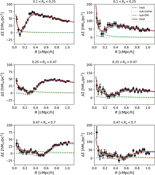
We present the galaxy–galaxy lensing signal of satellite galaxies in different Rp bins, along with their corresponding best-fitting models in Fig. 2. The excess surface mass density ΔΣ(R) of the cluster sample is represented by black circles with error bars, where the error bars reflect the 68 per cent confidence intervals obtained using jackknife resampling. The best-fitting models are shown as red solid lines, and the different components of the best-fitting model are represented by orange (stellar component), green (subhalo dark matter), and blue (host halo) lines, respectively. The model fitting results are listed in Table 1. The fitted value of the host halo normalization parameter α is very close to 1, indicating that the host halo contribution is very well described.
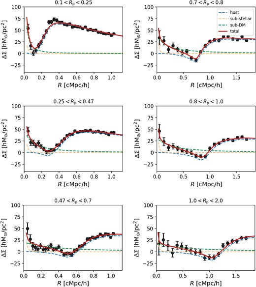
This figure shows the stacked galaxy–galaxy subhalo lensing signal for each Rp bin and the corresponding best-fitting model. The observed excess surface mass density ΔΣ(R) is represented by black circles with error bars, where the error bars reflect the 68 per cent confidence intervals obtained using the jackknife resampling method. The best-fitting model is shown as red lines, with the subhalo dark matter term represented by green lines, the stellar mass contribution from the satellite galaxy represented by orange lines, and the contribution from the host dark matter halo term represented by blue lines.
We present the SHMR for each satellite bin in Fig. 3. The solid red circles linked by a dashed line represent the fiducial results, which show that the SHMR increases with projected physical cluster-centric radius, from |$M_{\rm enh}/M_*=4.87_{-1.08}^{+1.15}$| at |$R_{\rm pp} =0.13~{\rm Mpc}\, h^{-1}$|, to |$76.78^{+36.54}_{-28.75}$| at |$R_{\rm pp}=0.89~{\rm Mpc}\, h^{-1}$|. This increase in SHMR reflects the significant mass-loss experienced by subhaloes after they fall into the host halo, likely due to tidal stripping effects.
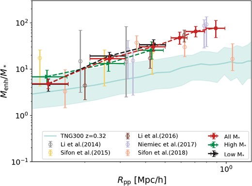
This figure shows the evolution of SHMR of satellite galaxies with an increase of projected physical cluster-centric distance Rpp. The red circles with error bars denote the best-fitting SHMR measurement of this work. The green right triangle and black left triangle show the SHMR of our high-M* and low-M* subsamples. We compare our fitting result with the SHMR in TNG300 simulation of the IllustrisTNG project. The solid line represents the median and mean value of SHMR, and the upper and lower boundaries of the shaded area represent the 16th and 84th percentile. The other empty circles with error bars are the SHMR results from previous satellite galaxy–galaxy lensing observations (Li et al. 2014, 2016a; Sifón et al. 2015, 2018; Niemiec et al. 2017).
For the inner three Rp bins, we split the satellite galaxies into high-M* (green triangles) and low-M* (black triangles) subsamples. See Appendix B for detailed subsample binning. We list the best-fitting model parameters for each subsample in Table 2, and the corresponding lensing signals are shown in Fig. B1. Although the subhalo masses of the high-M* subsample are systematically higher than those of the low-M* subsample within the same Rp range, we find no significant difference between the two subsamples in terms of the SHMR.
In Fig. 3, we have plotted the observational results from various literature sources, and our results agree with those from Li et al. (2016a) and Niemiec et al. (2017), where a trend of increasing SHMR with projected halo-centric radius was observed. On the other side, Sifón et al. (2015) found that SHMR has only a weak dependence on Rpp and Sifón et al. (2018) showed an anti-U shaped trend of SHMR–Rpp. It should be noted that the redMaPPer cluster catalogue, which includes only red-sequence galaxies, was used in Li et al. (2016a), Niemiec et al. (2017), and this work, whereas Sifón et al. (2015, 2018) did not restrict the colour of member galaxies, and the galaxies in Sifón et al. (2018) have a much smaller mean stellar mass than those used in our study. However, it is unclear whether these differences in galaxy selection can account for the discrepancies shown in Fig. 3.
In Fig. 3, we also compare our observational results with the theoretical predictions from the state-of-art hydrodynamical simulation, TNG300-1 of the IllustrisTNG Project (Marinacci et al. 2018; Naiman et al. 2018; Nelson et al. 2018, 2019; Pillepich et al. 2018, 2019; Springel et al. 2018). We choose to use TNG300-1 simulation, which has a box size of ∼300 Mpc3, a dark matter mass resolution of 5.9 × 10⁷ M⊙, and a baryonic elements (stellar particles and gas cells) mass resolution of 1.1 × 10⁷ M⊙, where a statistical sample of analogues of redMaPPer clusters can be found. We select red satellite galaxies in TNG300 simulation whose stellar mass is larger than |$1\times 10^{10}\, {\rm M_{\odot }}\, h^{-1}$| and the corresponding main-halo mass M200c is larger than |${\rm 1\times 10^{14}\, {\rm M_{\odot }}\, \mathit{ h}^{-1}}$|, which precisely corresponds to the selection conditions of our observation samples, i.e. |$M_{*}\gt 10^{10}~{\rm M_{\odot }}\, h^{-1}$|, λ > 20. The definition of red galaxies is g − r > 0.5, where g and r are the magnitudes in the SDSS g band and r band of galaxies provided by TNG300. We chose to use the snapshot data at z = 0.32 because this snapshot is closest to the average redshift of all samples. In Fig. 3, the solid line presents the median value of SHMR (|$\frac{M_{\rm subfind}}{M_{*}}$|, Msubfind is the subfind subhalo mass), and the upper and lower boundaries of the shaded area represent the 16th and 84th percentile (i.e. the ±1σ confidence intervals). For the innermost Rp bin, our SHMR measurements are consistent with that of TNG300 simulation within 1σ error. For the other subsample bins, our measurements of SHMR are much higher than that of the simulation. In Appendix A, we demonstrate that the fitted subhalo mass from lensing signal, Menh, can effectively represent the subfind subhalo mass with TNG300-1 simulation data.
Following Niemiec et al. (2017), we calculate the mass-loss rate of satellite galaxies as
where Minfall represents the dark matter mass of the satellite galaxy before it falls into the galaxy cluster. In this project, we assume that the satellite galaxies have the same SHMR as those field galaxies before they fall into the galaxy clusters. We adopt the M*–SHMR for field galaxies derived by Shan et al. (2017) to calculate the Mh,
where lg(M1) = 12.52 ± 0.050, lg(M*,0) = 10.98 ± 0.036, β = 0.47 ± 0.022, δ = 0.55 ± 0.13, and γ = 1.43 ± 0.28 when 0.2 < z < 0.4. lg(M1) = 12.70 ± 0.057, lg(M*, 0) = 11.11 ± 0.038, β = 0.50 ± 0.025, δ = 0.54 ± 0.16, and γ = 1.72 ± 0.30 when 0.4 < z < 0.6. In the left panel of Fig. 4, we can see that the dark matter loss rate increases with decreasing projected cluster-centric distance of the satellite galaxies. The mass-loss rate of satellite galaxy subhaloes shows a clear dependence on their stellar mass. This difference becomes more pronounced at larger halo-centric radii. At a projection halo-centric radius of 0.5R200c, the lower mass subsample does not exhibit significant mass-loss, while the higher mass subsample has already lost over 80 per cent of its subhalo mass. However, at a projection halo-centric radius of 0.1R200c, both subsamples of satellite galaxies have lost over 80 per cent of their mass, with the higher mass subsample experiencing a mass-loss of over 90 per cent. Interestingly, the final SHMR does not exhibit a clear dependence on the stellar mass of the satellite galaxies (Fig. 3).
One caveat is that we assume that the stellar mass remains unchanged for the satellite galaxies as they spiral into the centre of the cluster. Smith et al. (2016) studied the co-evolution of dark matter and stars in satellite galaxies and found that the stars lose about 10 per cent of their mass when 80 per cent dark matter lost. If we take this effect into account, the satellite galaxies at the centre of the clusters should be compared with field galaxies with higher stellar mass, and as a result, these satellites should have an even higher mass-loss rate than presented here.
We compare the retain dark matter mass fraction Menh/Minfall with predictions from simulations in the right panel of Fig. 4. The red, green, and black lines represent the same subsamples as in the left panel. The orange circles with error bars represent the results from Xie & Gao (2015) with the Phoenix simulation (Gao et al. 2012). The solid orange circles represent the retained mass fraction of subhaloes with the present subhalo mass Msubfind to host halo mass Mh ratio ranging from 1 × 10⁻⁶ to 1 × 10⁻⁵ as a function of cluster-centric distance, while the empty circles represent the results for subhaloes with Msubfind/Mh > 1 × 10⁻⁵. We also plot theoretical predictions of Han et al. (2016) using the subgen code.6 We generated theoretical predictions for a galaxy cluster with |$M_{\rm 200c}=2.39 \times 10^{14}~{\rm M_{\odot }}\, h^{-1}$|, which is the average mass of our whole sample, along with the evolution of its subhaloes. Subhaloes are massive than 10−6M200c at the infall time. We select the satellite galaxies in this simulated galaxy cluster with |$M_{*}\gt 1\times 10^{10}~{\rm M_{\odot }}\, h^{-1}$|. The median, 16th, and 84th percentiles of the retained dark matter mass fraction of selected satellite galaxies are represented by the solid pink line and the dashed pink lines, respectively. The observed trend of retained mass fraction as a function of halo-centric radius is broadly consistent with theoretical expectations. However, in the innermost region of galaxy clusters, the observed retained mass is lower compared to the predictions of the Phoenix Cluster simulations, but it is in better agreement with Han et al. (2016). On the outskirts of galaxy clusters, the observed retained mass is similar to that from Phoenix Cluster but significantly higher than Han et al. (2016). The results suggest that future studies should include hydrodynamical simulations for comparison to better understand the discrepancies between observations and theory, as well as their implications for the process of galaxy formation.
In previous figures, we bin the satellite galaxies according to their projected halo-centric distances. In this project, we also try to stack satellite galaxies of all Rp, while binning the sample according to their stellar mass as shown in Appendix C. The lensing signal and the best-fitting model for each of these five subsamples are shown in Fig. C2. The average Rp values of five stellar mass bins are similar, with values of 0.33, 0.34, 0.36, 0.38, and 0.39 cMpc h−1, respectively. In Fig. 5, we plot the average stellar mass versus their subhalo mass in the left panel. The red solid line represents the function obtained by Niemiec et al. (2019) with satellite galaxies at redshift z = 0.35 in the Illustris-1 simulation. The brown solid line represents the best-fitting model for the stellar mass and dark matter mass of satellite galaxies at z = 0.24 in TNG300, as fitted by Niemiec et al. (2022). The green solid line corresponds to the fitted relationship between the stellar and dark matter masses for central/field galaxies (Shan et al. 2017). The orange (blue) solid line shows the relation between stellar mass and dark halo mass of satellite galaxies with weak gravitational lensing (Dvornik et al. 2020). In the right panel, we show the dark matter strip rate versus stellar mass with black solid circles with error bars. The average stripping rate is lowest for satellite galaxies of |${\sim} 4 \times 10^{10}~{\rm M_{\odot }}\, h^{-1}$| with |$\tau _{\rm strip}=0.59^{+0.10}_{-0.12}$|, and increase to |$\tau _{\rm strip}=0.91_{-0.02}^{+0.02}$| for the most massive bin of |$\left\langle M_*\right\rangle \sim 1.5 \times 10^{11}~{\rm M_{\odot }}\, h^{-1}$|. The orange solid circles represent the strip rate of satellite galaxies in Illustris-1 with stellar masses between 2 × 10⁷ and |$2 \times 10^{11}~{\rm M_{\odot }}\, h^{-1}$|, and the horizontal grey line shows the average strip rate of satellite galaxies in Illustris-1 calculated by Niemiec et al. (2019). The dark violet line shows the average dark matter stripping rate of passive satellite galaxies in TNG300 and the pink line shows that of all satellite galaxies, both results come from Niemiec et al. (2022). The dark blue solid line represents the theoretical value of dark matter strip rate obtained by a theoretical model that combines the abundance matching technique with the halo occupation distribution and conditional luminosity (or stellar mass) function from Rodríguez-Puebla, Avila-Reese & Drory (2013). Results of Niemiec et al. (2019) indicate that the average strip rate is nearly independent of the stellar mass, while the results of Rodríguez-Puebla, Avila-Reese & Drory (2013) show a decrease in the loss of dark matter mass for larger stellar mass, which is opposite to our observation results.
5 SUMMARY AND CONCLUSIONS
In this paper, we have performed galaxy–galaxy lensing analysis for satellite galaxies in redMaPPer galaxy clusters, derived the subhalo mass of these satellite galaxies as a function of projected halo-centric radius, and calculated the mass stripping rate of satellite galaxies. We obtain the following conclusions.
We find Menh/M* decreases significantly with decreasing projected halo-centric radius, reaching |$4.87^{+1.15}_{-1.08}$| at |$R_{\rm pp}=0.13~{\rm Mpc}\, h^{-1}$|, indicating dramatic mass-loss due to stripping of the host halo. Our results at confirm conclusions from previous measurements of redMaPPer cluster satellite galaxy samples and galaxy–galaxy lensing (Li et al. 2016a; Niemiec et al. 2017) at a higher S/N (see Fig. 3).
We provide the first measurement of the variation of dark matter mass-loss rate as a function of projected halo-centric distance. Previously, this variation could only be obtained through simulations or abundance matching. We find satellite galaxies with larger stellar masses lose more dark matter and have higher dark matter strip rates at the same projected radius. The difference in dark matter strip rates between high-M* and low-M* subsamples decreases as Rpp decreases. At positions very close to the cluster centre (∼0.1 × R200c), the dark matter mass-loss rate for all satellite galaxies reaches |${\sim} 80{{\ \rm per\ cent}}$|. On the other hand, the SHMR of satellite galaxies does not depend on the stellar mass of the satellite galaxies (see Fig. 4).
We find that the average dark matter stripping rate for satellite galaxies is approximately |${\sim} 73{{\ \rm per\ cent}}$|. The stripping rate is lowest for satellite galaxies with |$\left\langle M_*\right\rangle \sim 4 \times 10^{10}~{\rm M_{\odot }}\, h^{-1}$| and increases with M* for more massive satellite galaxies, reaching |${\sim} 91{{\ \rm per\ cent}}$| for satellite galaxies with |$\left\langle M_*\right\rangle \sim 1.5 \times 10^{11}~{\rm M_{\odot }}\, h^{-1}$|. While our results broadly agree with the theoretical predictions from the Illustris-1 simulation, we reveal a variation of the stripping rate as a function of stellar mass, which is not seen in the simulation (see Fig. 5).
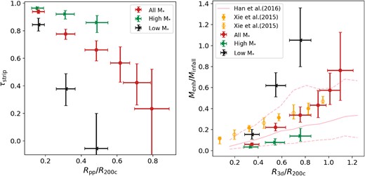
Left: Mass-loss rate of dark matter as a function of projected physical cluster-centric distance Rpp. The red solid circles with error bars represent our results of subsamples without binning by stellar mass, while the green triangles and black triangles represent the measurements for high-M* and low-M*, respectively. Right: The remained dark matter fraction as a function of three-dimensional cluster-centric distance R3d scaled with R200c, with the same colour scheme as in the left panel. The orange circles with error bars represent the Phoenix N-body simulation results taken from Xie & Gao (2015). The pink solid line and dashed line are from Han et al. (2016), representing the median value of SHMR and ±1σ confidence intervals, respectively.
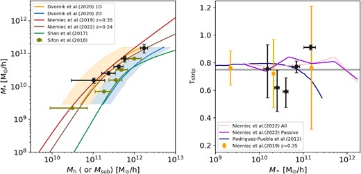
Left panel: Relation between dark matter mass and stellar mass. The black solid circles with error bars represent the results of subsamples binned by M* (see Appendix C for detailed sample binning). The red line represents the best-fitting relation for dark matter mass and stellar mass of subhaloes at z = 0.35 in Illustris-1 (Niemiec et al. 2019). The brown solid line represents the best-fitting model for the stellar mass and dark matter mass of satellite galaxies at z = 0.24 in TNG300 fitted by Niemiec et al. (2022). The green solid line represents the relation obtained by gravitational lensing measurements for the central/field galaxies in terms of their dark matter mass and stellar mass (Shan et al. 2017). The orange (blue) solid line shows the relation between stellar mass and dark halo mass of satellite galaxies with weak gravitational lensing (Dvornik et al. 2020). Right panel: Scatter plot of dark matter stripping rate versus stellar mass. The orange solid circles with error bars represent the average dark matter stripping rate of satellite galaxies with stellar masses between |$2 \times 10^{7}~{\rm M_{\odot }}\, h^{-1}$| and |$2 \times 10^{11}~{\rm M_{\odot }}\, h^{-1}$| in Illustris-1 at z = 0.35. The grey horizontal line represents the average dark matter stripping rate of all satellite galaxies in Illustris-1 measured by Niemiec et al. (2019). The dark violet line shows the average dark matter stripping rate of passive satellite galaxies in TNG300 and the pink shows that of all satellite galaxies, both results come from Niemiec et al. (2022). The dark blue solid line represents the theoretical value of the dark matter stripping rate obtained by Rodríguez-Puebla, Avila-Reese & Drory (2013).
These results demonstrate that satellite galaxy–galaxy lensing is a crucial tool to understand the co-evolution of galaxies and dark matter haloes. The next generation of galaxy surveys, such as the Euclid (Laureijs et al. 2011), the Vera Rubin Legacy Survey of Space and Time (LSST; Ivezić et al. 2019; Bianco et al. 2021), and the China Space Station Telescope (CSST; Zhan 2011, 2021), will provide one order of magnitude larger samples of background galaxies suitable for weak lensing analysis than the current DECaLs survey. These upcoming surveys will allow us to more accurately measure the evolution of satellite subhalo properties in various dark matter haloes.
Number of lenses in each subsample. The bins are separated with the M*, as shown in the first column. In the following columns, the parameters of each bin are listed in sequence, the number of lenses of subsample, the average redshift, the average projection cluster-centric physical distance, the average comoving projection cluster-centric physical distance, the average stellar mass, host halo normalization α, subhalo mass, SHMR, and average dark matter strip rate. All the masses are in unit of |${\rm M_{\odot }}\, h^{-1}$| and distance in Mpc h−1.
| lg(M*) range | Num | <z> | <Rpp> | <Rp> | lg(<M*>) | α | rsub | lg(Menh) | Menh/<M*> | τstrip |
|---|---|---|---|---|---|---|---|---|---|---|
| 10.0–10.3 | 421 86 | 0.3 | 0.25 | 0.33 | 10.19 | |$1.04_{-0.02}^{+0.01}$| | |$0.05_{-0.02}^{+0.02}$| | |$11.01_{-0.55}^{+0.27}$| | |$6.71_{-4.8}^{+5.78}$| | |$0.76_{-0.21}^{+0.17}$| |
| 10.3–10.5 | 513 29 | 0.31 | 0.26 | 0.34 | 10.41 | |$1.01_{-0.03}^{+0.01}$| | |$0.07_{-0.01}^{+0.02}$| | |$11.38_{-0.18}^{+0.16}$| | |$9.37_{-3.13}^{+4.23}$| | |$0.62_{-0.17}^{+0.13}$| |
| 10.5–10.7 | 517 36 | 0.32 | 0.27 | 0.36 | 10.6 | |$0.98_{-0.02}^{+0.02}$| | |$0.09_{-0.01}^{+0.01}$| | |$11.62_{-0.12}^{+0.11}$| | |$10.41_{-2.53}^{+3.0}$| | |$0.59_{-0.12}^{+0.1}$| |
| 10.7–11.0 | 578 28 | 0.33 | 0.29 | 0.38 | 10.84 | |$0.98_{-0.01}^{+0.01}$| | |$0.09_{-0.01}^{+0.01}$| | |$11.76_{-0.08}^{+0.08}$| | |$8.36_{-1.45}^{+1.66}$| | |$0.77_{-0.05}^{+0.04}$| |
| 11.0–11.5 | 262 41 | 0.34 | 0.3 | 0.39 | 11.17 | |$0.96_{-0.03}^{+0.03}$| | |$0.15_{-0.02}^{+0.02}$| | |$12.24_{-0.09}^{+0.09}$| | |$11.67_{-2.16}^{+2.55}$| | |$0.91_{-0.02}^{+0.02}$| |
ACKNOWLEDGEMENTS
We acknowledge the support by National Key R&D Program of China no. 2022YFF0503403, the support of National Nature Science Foundation of China (nos 11988101, 12022306), the support from the Ministry of Science and Technology of China (no 2020SKA0110100), the science research grants from the China Manned Space Project (nos CMS-CSST-2021-B01, CMS-CSST-2021-A01), CAS Project for Young Scientists in Basic Research (no. YSBR-062), and the support from K.C. Wong Education Foundation. HS acknowledges the support from NSFC under grant no. 11973070, Key Research Program of Frontier Sciences, CAS, grant no. ZDBS-LY-7013, and Program of Shanghai Academic/Technology Research Leader. We acknowledge the support from the science research grants from the China Manned Space Project with nos CMS-CSST-2021-A01, CMS-CSST-2021-A04. WX acknowledges support from the National Science Foundation of China (11721303,11890693,12203063) and the National Key R&D Program of China (2016YFA0400703). JY acknowledges the support from NSFC grant no. 12203084, the China Postdoctoral Science Foundation grant no. 2021T140451, and the Shanghai Post-doctoral Excellence Program grant no. 2021419.
DATA AVAILABILITY
The data underlying this article will be shared on a reasonable request to the authors.
Footnotes
References
APPENDIX A
To validate our method with simulation data, we selected red satellite galaxies with g − r > 0.5, |$M_{*}\gt 1\times 10^{10}\, {\rm M_{\odot }}\, h^{-1}$| and the corresponding main-halo mass M200c is larger than |${\rm 1\times 10^{14}\, {\rm M_{\odot }}\, \mathit{ h}^{-1}}$| from the TNG300-1 simulation at z = 0.32. We binned the satellite galaxies based on their projected halo-centric radius Rp on the x–y plane or by their stellar mass M*. By stacking the satellite–central galaxy pairs, we obtained the excess surface density ΔΣ(R), and subsequently, we derived subhalo mass Menh by fitting this gravitational lensing signal with the same method as we did for the observational lensing signal. We compare Menh with the corresponding average subfind mass Msubfind of each subsample. The comparison results of Rp binned subsamples and M* binned subsamples are presented in Figs A1 and A2. In both figures, black dots represent the subhalo mass, Menh, obtained from fitting the lensing signal, while the red solid dots represent the corresponding average subfind subhalo mass |$\overline{M}_{\rm subfind}$|. The grey shaded area represents the 1σ confidence interval of Menh, which is estimated from the relative error of subhalo mass obtained by fitting the real observational data from the corresponding subsamples. As we can see that Menh and |$\overline{M}_{\rm subfind}$| are consistent within 1σ confidence interval and the relative deviations |$\frac{M_{\rm enh}-\overline{M}_{\rm subfind}}{\overline{M}_{\rm subfind}}$| are within ±16 per cent for the vast majority of subsamples, indicating that the fitted subhalo mass from lensing signal can effectively represent the subfind subhalo mass.
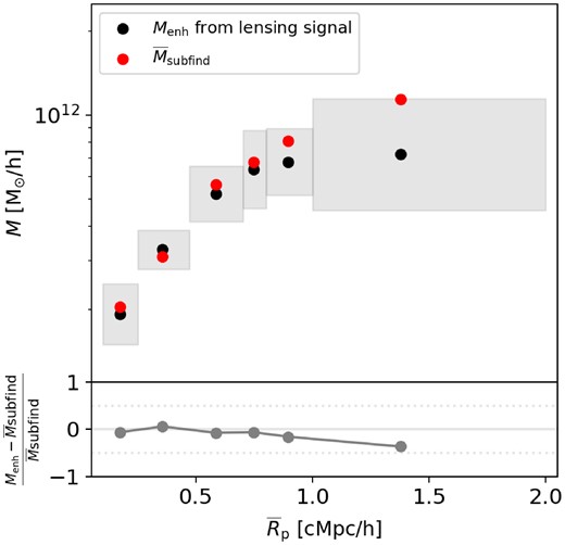
Comparison between subhalo mass Menh derived from lensing signals and the average value of subfind mass, |$\overline{M}_{\rm subfind}$|. In the upper subplot, black solid circles represent subhalo mass Menh derived from lensing signals, while red solid circles indicate |$\overline{M}_{\rm subfind}$|. The grey shaded area represents the 1σ error of Menh, which is estimated from the relative error of subhalo mass obtained by fitting the real observational data from the corresponding subsamples. The lower subplot illustrates the variation of |$\frac{M_{\rm enh}-\overline{M}_{\rm subfind}}{\overline{M}_{\rm subfind}}$| with the averaged projected halo-centric radius |$\overline{R}_{\rm p}$|. The solid grey line represents y = 0. The two grey dotted lines represent y = 0.5 and y = −0.5.

Similar to Fig. A1, this figure shows the results of subsamples binned by stellar mass M*. The horizontal axis represents the average stellar mass of subsamples.
APPENDIX B
To test whether the SHMR depends on stellar mass, we divide each of the smallest three Rp subsample in Section 2.1 into two subsamples, namely high-M* (|$10^{11}\, {\rm M_{\odot }}\, h^{-1} \lt M_{*}\lt 10^{12}\, {\rm M_{\odot }}\, h^{-1}$|) and low-M* (|$10^{10}\, {\rm M_{\odot }}\, h^{-1} \lt M_{*}\lt 10^{11}\, {\rm M_{\odot }}\, h^{-1}$|) subsamples. Here, we present the gravitational lensing signals and the best-fitting model of the high-M* and low-M* subsamples in Fig. B1. The number of lenses and best-fitting parameters of each subsample are listed in Table 1.
Similar to Fig. 2, but here we show the lensing signals and best-fitting models corresponding to the low-M* (left column) and high-M* (right column) subsamples.
APPENDIX C
To obtain the average dark matter stripping rate of satellite galaxies in different stellar mass ranges, we divided the sample with stellar masses ranging from |$10^{10}~{\rm M_{\odot }}\, h^{-1}$| to |$10^{11.5}~{\rm M_{\odot }}\, h^{-1}$| and satisfying the criteria of 0.1 < z < 0.5, Pmem > 0.8, |${\rm 0.1~cMpc}\, h^{-1}\lt R_{\rm p}\lt {\rm 1.0~cMpc}\, h^{-1}$|, and DEC < 34 into five subsamples. The distributions of stellar mass, redshift, and comoving lensing distance to the central galaxy for each subsample are shown in Fig. C1, with the same colour used to represent the same subsample in all three panels. The five subsamples have very similar redshift distributions, and the Rp distributions of the four lower stellar mass bins are also very similar. However, the subsample with the largest stellar mass has a relatively larger Rp projection distance. The bin edges of the stellar mass and the corresponding number of satellite galaxies in each bin, as well as the best-fitting model parameters, are listed in Table 2.
We also use the swot software to calculate the lensing signals for different subsamples (60 linear radial bins, |$0.05~{\rm cMpc}\, h^{-1}\lt R\lt 1.75~{\rm cMpc}\, h^{-1}$|), and fit the lensing signals with MCMC sampler emcee. The lensing signals and best-fitting models of different subsamples are shown in Fig. C2.
Similar to Fig. 1, here we show the histogram distributions of stellar mass M*, redshift z, and comoving lensing distance Rp for subsamples binned solely based on M*. The same subsamples are represented with consistent colours across the three panels.
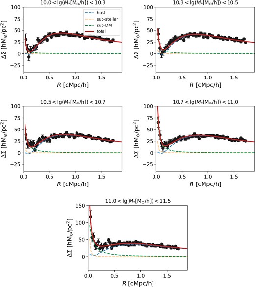
Similar to Fig. 2, here we show the lensing signal and the best-fitting model of subsamples binned solely based on M*.
