


ABSTRACT
The core-shift method is a powerful method to estimate the physical parameters in relativistic jets from active galactic nuclei. The classical approach assumes a conical geometry of jets and a constant plasma speed. However, recent observations have shown that neither may hold close to the central engine, where the plasma in the jet is effectively accelerating and the jet geometry is quasi-parabolic. We modify the classical core-shift method to account for these jet properties. We show that the core-shift index may assume values in the range 0.8−1.2 or 0.53−0.8 depending on the jet geometry and viewing angle, and indices close to both values are indeed observed. We obtain expressions to estimate the jet magnetic field and the total magnetic flux in a jet. We show that the obtained magnetic field value can be easily recalculated down to the gravitational radius scale. For M87 and NGC 315, these values are in good agreement with those obtained by different methods.
1 INTRODUCTION
It is now generally accepted as a model that the ordered magnetic field in the vicinity of supermassive black holes (BHs) residing in the centres of active galactic nuclei plays the key role in launching relativistic jets (Blandford, Meier & Readhead 2019). It is the presence of the magnetic field that either threads the BH ergosphere and establishes the Blandford–Znajek process (Blandford & Znajek 1977), responsible for the extraction of BH rotational energy to supply the jet power (Tchekhovskoy, Narayan & McKinney 2011), or launches the jet from the disc via the Blandford–Payne mechanism (Blandford & Payne 1982). The Poynting flux at the jet base defines the maximum Lorentz factor that can be achieved if all the energy of the electromagnetic field is transformed into plasma bulk motion kinetic energy (e.g. Beskin 2010).
Many efforts have been made to understand the magnitude and geometry of the jet magnetic field at different scales. Polarization measurements in the radio band yield information about the possible B-field geometry. Multiple studies at parsec scales have revealed the helical magnetic field expected from theoretical modelling (Gabuzda et al. 2017; Gabuzda, Nagle & Roche 2018). The unprecedented radio images of M87 confirmed that the helical magnetic field B is maintained at scales from 300 pc up to 1 kpc (Pasetto et al. 2021). The phenomenon of the observed Faraday rotation measure (RM) changing sign can be explained by the presence of a toroidal magnetic field around the jet in 3C 273 up to distances of the order of 500 pc de-projected (Lisakov et al. 2021). The detection of a large-scale toroidal magnetic field at kiloparsec scales (Knuettel, Gabuzda & O’Sullivan 2017) indicates the strong electric current flowing in relativistic jets far from the expected acceleration and collimation domain (Blandford, Meier & Readhead 2019; Kovalev et al. 2020), showing the importance of the Poynting flux even at such distances from the central engine. Direct polarimetry of the event horizon scales in the M87 jet conducted by Event Horizon Telescope Collaboration (2021) gives the B-field magnitude to be of the order of a few to tens of gauss.
One of the most robust methods to estimate the magnetic field amplitude on an observational basis is to use core-shift measurements. The core-shift effect is observed in jets owing to the changing physical properties (flow velocity, magnetic field, and emitting-plasma number density) along an outflow, so that the surface with optical depth equal to unity appears at different positions for different observational frequencies (Lobanov 1998; Hirotani 2005). Together with the model assumptions, core-shift measurements provide typical values for the magnetic field of the order of 1 G at 1-pc distance (Lobanov 1998). The results obtained using this method are in general agreement with other expected jet parameters, such as initial magnetization and jet composition (Hirotani 2005; O’Sullivan & Gabuzda 2009; Pushkarev et al. 2012; Nokhrina et al. 2015; Zdziarski et al. 2015).
The core-shift method as its important ingredients makes the following assumptions: equipartition between the proper-frame emitting particles and the magnetic field energy density, certain scalings with the distance of the magnetic field B and plasma number density n (Blandford & Königl 1979), and a conical jet geometry. The observed jet boundary shape – the dependence of the jet width d on the distance along a jet r – can be approximated by the power law
An extensive study of jet shapes (see e.g. Pushkarev et al. 2017, and references within) reveals an approximately constant power k ≈ 1 in many sources, corresponding to a conical or quasi-conical geometry. However, recent studies of a dozen nearby jets demonstrate that their shapes are consistent with two power laws, smoothly transitioning from one to another on a more or less short scale of the overall length range (Asada & Nakamura 2012; Tseng et al. 2016; Akiyama et al. 2018; Hada et al. 2018; Nakahara et al. 2018, 2019; Kovalev et al. 2020; Nakahara et al. 2020; Boccardi et al. 2021; Park et al. 2021; Okino et al. 2022). For these sources, typical values of k closer to the jet launching point are in the range k ≈ 0.39−0.59. We refer to this as quasi-parabolic, or parabolic for short. Further downstream, the shape becomes closer to conical (quasi-conical), with k ≈ 0.73−1.4 (e.g. Asada & Nakamura 2012; Kovalev et al. 2020; Boccardi et al. 2021). The implicit study of the geometry of more distant sources, which uses the plasma velocity instead of the direct measurements of a jet shape, shows that cores at 15 and 8 GHz belong to the quasi-parabolic part of a jet (Nokhrina, Pashchenko & Kutkin 2022). This means that one may expect the radio cores observed at high frequencies 230−15 GHz, and maybe down to 8 GHz, to be in the parabolic domain and with the plasma still being accelerated. This may impact the results obtained by the classical core-shift method, which uses typical observational frequencies of 8–15 GHz (Pushkarev et al. 2012).
The parabolic accelerating jet model alters the kr-index in the frequency dependence of the core position |$r_\mathrm{core}\propto \nu ^{-1/k_\mathrm{r}}$| (Ricci et al. 2022). Multifrequency observations for M87 by Hada et al. (2011) and for 20 sources by Sokolovsky et al. (2011) demonstrate that kr is indeed close to unity. This may be explained either by the conical jet model with a constant Lorentz factor Γ, which may be the case for the sample by Sokolovsky et al. (2011), or by the quasi-parabolic accelerating jet model observed at the maximum Doppler factor (Ricci et al. 2022) for the M87 jet with a clear quasi-parabolic shape. On the other hand, a dedicated search in NGC 315 by Ricci et al. (2022) yielded a change in the kr- index from 0.57 to 0.93 at approximately the jet-shape transition point. Using different methods, Kutkin et al. (2014) found the exponent kr in the range 0.6–0.8 for quasar 3C 454.3. The typical kr-index for the MOJAVE (Monitoring Of Jets in Active galactic nuclei with Very Long Baseline Array Experiments) sample was estimated to be approximately 0.83 by Kravchenko et al. (in preparation).
Accounting for parabolic accelerating jets alters the scalings of the magnetic field B and plasma number density n as functions of distance from the central source r, introduces the non-constant plasma bulk flow motion Lorentz factor Γ, and changes the way of extrapolating the magnetic field amplitude down to the gravitational radius scale (Ricci et al. 2022). In this paper, we modify the core-shift method for a parabolic jet boundary geometry and estimate the magnetic filed amplitude at the gravitational radius for 10 sources.
The paper is organized as follows. In Section 2 we present the model for the magnetic field and emitting-particle number density to obtain the possible core-shift indices kr for parabolic accelerating jets. In Section 3 we discuss the relationship between the magnetic field and plasma number density and obtain expressions to estimate both values. In Section 4 we review the data to estimate B. We discuss our results and methods in Section 5. Finally, we summarize our work in Section 6.
2 FREQUENCY-DEPENDENT APPARENT CORE SHIFT IN A PARABOLIC ACCELERATING FLOW
The emission and opacity of a jet results from the emitting-plasma population with an assumed power-law energy distribution in the plasma proper frame, designated by the asterisk:
where α is the power of the spectral flux in the optically thin regime: Sν ∝ ν−α. Here, Ke* is the amplitude of the emitting-plasma energy distribution:
The relationship between the observational frequency ν and the local properties of a jet at the surface of the peak spectral flux (which approximately coincides with the surface with the optical depth equal to unity) is as follows (e.g. equation 21 in Hirotani 2005):
Here m, e, c, r0 are the electron mass and charge, the speed of light, and the classical electron radius, respectively; ν0 = c/r0; and C1(0.5) = 2.85 for α = 0.5 (Gould 1979). The local jet width is d, the emitting-electron number density amplitude is Ke*, and the local magnetic field in the plasma proper frame is B*. The jet viewing angle is θ, and the Doppler factor for a bulk Lorentz factor Γ = (1 − β2)−0.5 is
In order to obtain the dependence of the core position on the observational frequency, we need to set the dependence of Ke*, B*, Γ, d, and δ on the distance along the jet r.
The typical frequencies for the core-shift measurements are 1.4−43 GHz (Kovalev et al. 2008; Hada et al. 2011; Sokolovsky et al. 2011; Boccardi et al. 2021) and may be as high as 86 and 230 GHz for M87 (Doeleman et al. 2012; Hada et al. 2016). This means that either all the observational frequencies or the highest ones may probe the jet in its parabolic accelerating domain. Thus, we assume here that the jet shape is given by (1), with the value for power k = 0.5 for a strictly parabolic outflow, and k ≈ 0.4−0.6 for a quasi-parabolic one.
In general, we assume the power laws |$K_{\rm e*}\propto r^{-k_\mathrm{n}}$| and |$B_*\propto r^{-k_\mathrm{b}}$|. The magnetic field in a jet is decomposed into poloidal Bp and toroidal Bφ components. The toroidal component dominates the major part of the jet, r > RL, as there is a universal relationship Bφ = Bpr/RL for a relativistic flow (see e.g. Lyubarsky 2009). However, as the velocity of the bulk plasma motion is dominated by the poloidal component, the corresponding relationship in the plasma proper frame between Bp* ≈ Bp and |$B_{\varphi *}\approx \sqrt{B_{\varphi }^2-E^2}$| can be different. We focus on the domain where the jet plasma is still effectively accelerating. In this case, either the co-moving magnetic field is dominated by the poloidal component |$B_\mathrm{p}^2\gg B_{\varphi }^2-E^2$| or both components in the plasma proper frame are comparable, namely |$B_\mathrm{p}^2\sim B_{\varphi }^2-E^2$| (Vlahakis 2004; Komissarov et al. 2009). In this case, we adopt
To keep the final expression as simple as possible we will not account here for the jet transversal structure. Thus, the conservation of the total magnetic flux defines the dependence of B* on the distance r:
where rζ is the distance at which we will estimate the magnetic field and the emitting-plasma number density. It is convenient to use rζ = 1 pc, except for sources with the jet shape break detected at smaller distances, as in NGC 315 (Boccardi et al. 2021; Ricci et al. 2022).
The plasma number density obeys the continuity equation and can be written as
for the steady state in an accelerating jet. Here, subscripts 1 and 2 indicate two different crosscuts perpendicular to the jet axis. We expect that the jets are still effectively accelerating in the parabolic domain (Nokhrina et al. 2019; Kovalev et al. 2020; Nokhrina, Kovalev & Pushkarev 2020; Nokhrina, Pashchenko & Kutkin 2022), and the plasma bulk motion Lorentz factor
increases linearly with the jet radius d/2 and depends on the light cylinder radius RL (Beskin & Nokhrina 2006; Komissarov et al. 2007; Lyubarsky 2009). The ideal linear acceleration, Γ ∝ d, is valid while the flow is still highly magnetized. In order to account for the slowing down of this Lorentz factor behaviour as the flow approaches the saturation state with the magnetization equal to unity, we introduce the coefficient ρ. Using relationship (A13) from Nokhrina, Pashchenko & Kutkin (2022) and table 1 from Nokhrina et al. (2019), we conclude that ρ ≈ 0.3–0.55. Using (8) and (9), we obtain the following relationship for the emitting-plasma number density amplitude:
Parameters of the sources with a measured parabolic jet shape and core shift.
| Source | z | θ | θ | M | M | δ | φapp |
|---|---|---|---|---|---|---|---|
| (°) | Reference | (log M⊙) | Reference | (°) | |||
| (1) | (2) | (3) | (4) | (5) | (6) | (7) | (8) |
| 0055+300 | 0.017 | 38.0 | Ricci et al. (2022) | 9.32 | Boizelle et al. (2021) | ... | 6.9 |
| 0111+021 | 0.047 | 5.0 | Kovalev et al. (2020) | ... | ... | ... | 9.3 |
| 0415+379 | 0.049 | 17.4 | Pushkarev et al. (2017) | 8.21 | Torrealba et al. (2012) | 2.9 | 7.9 |
| 0430+052 | 0.033 | 18.7 | Pushkarev et al. (2017) | 8.13 | Woo & Urry (2002) | 5.9 | 9.6 |
| 1226+023 | 0.158 | 3.3 | Pushkarev et al. (2017) | 8.41 | Gravity Collaboration et al. (2018) | 17.0 | 6.6 |
| 1228+126 | 0.004 | 18.0 | Nakamura et al. (2018) | 9.82 | EHT Collaboration et al. (2019) | 3.2* | 12.0 |
| 1514+004 | 0.052 | 15.0 | Kovalev et al. (2020) | ... | ... | ... | 7.3 |
| 1637+826 | 0.024 | 18.0 | Kovalev et al. (2020) | 8.78 | Ferrarese & Ford (1999) | ... | 7.2 |
| 1807+698 | 0.051 | 7.3 | Pushkarev et al. (2017) | 8.51 | Woo & Urry (2002) | 1.1 | 10.6 |
| 2200+420 | 0.069 | 8.0 | Pushkarev et al. (2017) | 8.23 | Woo & Urry (2002) | 7.3 | 24.8 |
Notes. The columns are as follows: (1) source name (B1950); (2) redshift (collected by Kovalev et al. 2020); (3) viewing angle; (4) viewing angle reference; (5) black hole mass; (6) black hole mass reference; (7) variability Doppler factor from Hovatta et al. (2009); (8) apparent opening angle at 15-GHz core by Pushkarev et al. (2017).
* For 1228+126, the Doppler factor is based on the velocities at parsec scale measured by Mertens et al. (2016) and the viewing angle.
Substituting (7) and (10) into (4), we obtain the relationship for the frequency-dependent core position:
For the different relationships between the viewing angle θ and local Lorentz factor Γ in Ricci et al. (2022), we obtain three different values of the core-shift exponent kr. For θ ≈ Γ−1, the Doppler factor is approximately constant, and
For kn = 3k and kb = 2k, the core-shift exponent does not depend on the index of the emitting-particle distribution α: kr = 2k. If θ ≪ Γ−1, the Doppler factor is proportional to the Lorentz factor δ ≈ 2Γ, and
Substituting exponents from (7) and (10), we obtain
This expression depends weakly on the emitting-particle distribution for a reasonable range of α (see e.g. Gould 1979). For α = 0.5, this exponent kr = 4k/3. If θ ≫ Γ−1 and δ ∝ Γ−1, one obtains
For kn = 3k and kb = 2k,
which is equal to kr = 8k/3 for α = 0.5 and, again, in general depends on α very weakly. All the above results were obtained by Ricci et al. (2022), but assuming the dominance of the toroidal magnetic field in the collimation and acceleration region.
Obtained above value kr = 2k for θ ≈ Γ−1 for a strictly parabolic power k = 0.5 provides kr = 1, which coincides with the result for a conical outflow with a constant speed. This value of kr index is supported by multifrequency measurements for a dozen sources (Hada et al. 2011; Sokolovsky et al. 2011). However, for different quasi-parabolic jet collimation profiles and different viewing angles, kr may vary. The core-shift exponent measurements for NGC 315 favour θ ≪ Γ−1 and kr = 4k/3 (Ricci et al. 2022).
It is convenient to use the core-shift offset (Lobanov 1998)
where Δrmas is the measured core shift in milliarcseconds for observational frequencies ν1 and ν2 for a source at the luminosity distance DL and corresponding cosmological redshift z. The core-position offset measure depends on Ke*ζ and B*ζ. If the relationship between Ke*ζ and B*ζ is set, the measured core shift allows estimation of the magnetic field and emitting-particle number density (Lobanov 1998; Hirotani 2005; O’Sullivan & Gabuzda 2009; Nokhrina et al. 2015).
3 MAGNETIC FIELD ESTIMATES BASED ON THE CORE-SHIFT EFFECT
The classical equipartition between the emitting plasma and magnetic field |$K_{e*}\propto B_{*}^2$| can no longer hold everywhere because of relationships (7) and (10) being incompatible with the conical approach (see Appendix A). To relate Ke*ζ and B*ζ we introduce the local magnetization – the ratio of the Poynting flux to the plasma bulk motion kinetic energy flux (see e.g. Nokhrina et al. 2015):
Setting σ = 1, which corresponds to Γ = Γmax/2, and using the universal relationship for relativistic flows between the toroidal and poloidal magnetic field components (e.g. Vlahakis 2004; Komissarov et al. 2009; Lyubarsky 2009), namely
we obtain
In order to relate the plasma number density and magnetic field at a given distance ζ and the point σ = 1, we use (7) and (10). This provides the following relationship for n*ζ and B*ζ:
Assuming that just a fraction |$\eta \in (0;\, 1]$| of all the plasma emits, we set
With the above relationship, we are able to write the final expression for estimating the jet magnetic field using the core-shift effect in the parabolic accelerating jet with δ ≈ const (kr = 2k):
In the expression for the magnetic field B*ζ, all the distances (rζ, dζ, dbr and RL) are in parsecs. It can be compared with the classical expression for a magnetic field in the plasma proper frame at a distance 1 pc from the jet base (e.g. Lobanov 1998; Hirotani 2005):
where φ is the intrinsic half-opening angle for a conical jet.
The expression for the magnetic field in the case of δ ≈ 2Γ (kr = 4k/3) can be written as:
Although the case of kr = 8k/3 (δ ∝ Γ−1) is unlikely, based on current observations, we still present the expression for B:
For the domain of effectively accelerating outflow, the co-moving magnetic field is dominated by the poloidal component (Vlahakis 2004; Komissarov et al. 2009). This makes it straightforward to estimate the total magnetic flux contained in a jet and to extrapolate the magnetic field down to the gravitational radius scale.
The total magnetic flux is estimated as
Using magnetic flux conservation, we obtain the magnetic field amplitude at the gravitational radius scale as
4 MAGNETIC FIELD ESTIMATES
Below we apply the above relationships to sources with measured jet shape and core shift. Additionally, we use the black hole mass estimate to assess the magnetic field amplitude at the gravitational radius. The required parameters are summarized in Tables 1–3.
Jet geometry parameters of the sources.
| Source | Alias | k | dbreak | rbreak | a1 | Geometry |
|---|---|---|---|---|---|---|
| (pc) | (pc) | (pc1 − k) | Reference | |||
| (1) | (2) | (3) | (4) | (5) | (6) | (7) |
| 0055+300 | NGC 315 | 0.45 | 0.072 | 0.58 | 0.092 | Boccardi et al. (2021); Ricci et al. (2022) |
| 0111+021 | UGC 00773 | 0.497 ± 0.077 | 0.28 | 27.31 | 0.179 ± 0.010 | Kovalev et al. (2020) |
| 0415+379 | 3C 111 | 0.468 ± 0.026 | 0.74 | 29.00 | 0.305 ± 0.011 | Kovalev et al. (2020) |
| 0430+052 | 3C 120 | 0.556 ± 0.070 | 0.29 | 5.77 | 0.202 ± 0.015 | Kovalev et al. (2020) |
| 1226+023 | 3C 273 | 0.66 | 3.0 | 274 | 0.223 | Okino et al. (2022) |
| 1228+126 | M 87 | 0.57 | 1.2 | 43.4 | 0.07 | Nokhrina et al. (2019) |
| 1514+004 | PKS B1514+004 | 0.564 ± 0.048 | 0.34 | 13.1 | 0.171 ± 0.019 | Kovalev et al. (2020) |
| 1637+826 | NGC 6251 | 0.506 ± 0.041 | 0.16 | 3.3 | 0.155 ± 0.005 | Kovalev et al. (2020) |
| 1807+698 | 3C 371 | 0.388 ± 0.087 | 0.25 | 12.8 | 0.207 ± 0.016 | Kovalev et al. (2020) |
| 2200+420 | BL Lac | 0.537 ± 0.057 | 0.95 | 24.6 | 0.505 ± 0.029 | Kovalev et al. (2020) |
Note. The columns are as follows: (1) source name (B1950); (2) k-index upstream the jet shape geometry transition (parabolic flow); (3) jet width in the trasnition region; (4) jet shape break position from the jet base; (5) a1 coefficient in the jet shape (parabolic flow); (6) reference for jet geometry results.
Opacity parameters of the sources and the locations of radio cores and jet shape break points.
| Source | Δr | ν1 | ν2 | Reference | Ωrν | |$r_{\nu _2}$| | |$r_{\nu _1}$| |
|---|---|---|---|---|---|---|---|
| (mas) | (GHz) | (GHz) | Nuclear opacity | |$(\mathrm{pc\, GHz}^{1/k_\mathrm{r}})$| | (pc) | (pc) | |
| (1) | (2) | (3) | (4) | (5) | (6) | (7) | (8) |
| 0055+300 | 0.420 | 8.4 | 15.4 | Boccardi et al. (2021) | 8.94 | 0.12 | 0.34 |
| 0111+021 | 0.137 | 8.1 | 15.4 | Pushkarev et al. (2012) | 2.15 | 1.57 | 3.00 |
| 0415+379 | 0.315 | 8.1 | 15.4 | Pushkarev et al. (2012) | 5.62 | 1.01 | 2.01 |
| 0430+052 | 0.075 | 8.1 | 15.4 | Pushkarev et al. (2012) | 0.729 | 0.19 | 0.35 |
| 1226+023 | 0.036 | 15.4 | 23.7 | Okino et al. (2022) | 2.76 | 4.36 | 6.04 |
| 1228+126 | 0.089 | 8.1 | 15.4 | Hada et al. (2011) | 0.113 | 0.028 | 0.051 |
| 1514+004 | 0.139 | 8.1 | 15.4 | Pushkarev et al. (2012) | 2.05 | 0.70 | 1.24 |
| 1637+826 | 0.210 | 8.1 | 15.4 | Pushkarev et al. (2012) | 1.70 | 0.37 | 0.69 |
| 1807+698 | 0.249 | 8.1 | 15.4 | Pushkarev et al. (2012) | 6.44 | 1.49 | 3.41 |
| 2200+420 | 0.032 | 8.1 | 15.4 | Pushkarev et al. (2012) | 0.645 | 0.37 | 0.66 |
Note. The columns are as follows: (1) source name (B1950); (2) core shift between low and high frequencies; (3) low frequency; (4) high frequency; (5) reference for core-shift measurement; (6) core-position offset Ωrν calculated using columns (2)–(4) and kr from Table (4); (7) core position from the jet base at the high frequency assuming kr from Table 4; (8) as column (7) but for low frequency.
To calculate the parameter Ωrν using expression (17) we adopt the core-shift measurements by Pushkarev et al. (2012) between the observational frequencies of 15.4 and 8.1 GHz. We also set kr = 2k, where the power k in the parabolic regime was measured in Kovalev et al. (2020) (see Tables 2 and 4). For the M87 jet we use the core-shift measurements reported by Hada et al. (2011). The core position dependence is
For homogeneity of the results, we calculate the core shift between the pair of frequencies 8.1 and 15.4 GHz (see Table 3) using this expression. The kr-index obtained by Hada et al. (2011) assumes the value |$1.06^{+0.12}_{-0.09}$| and is in good agreement with the relationship kr = 2k, corresponding to a constant Doppler factor result (12). We set the measured kr = 1.06 for M87 (Hada et al. 2011). For NGC 315 we use the recent results by Ricci et al. (2022). In particular, multifrequency measurements are consistent with kr = 0.57 ± 0.17 at 22−8 GHz, and with kr = 0.92 ± 0.01 at 8−5 GHz. This result is in agreement with formula (14), kr = 4k/3, with 4k/3 = 0.6 for k = 0.45 (Boccardi et al. 2021). We adopt the core-shift measurement by Boccardi et al. (2021) between the frequencies of 15.4 and 8.4 GHz. For 3C273, the core shift was measured by Okino et al. (2022). We chose the pair 23.7 and 15.4 GHz as the closest to the frequency pair in other sources. We also adopt kr = 2k, because the authors fitted the core shift with assumed kr = 1. The opacity parameters are listed in Table 3. Note that Ωrν here is calculated with kr, which differs from unity. In order to check that the corresponding cores are indeed lying in the quasi-parabolic domain, we calculated the positions of cores from a jet base at the high and low frequencies: |$r_{\nu _2}$| and |$r_{\nu _1}$| , as listed in columns (7) and (8) of Table 3. We see that these cores lie closer to the jet base than the geometry break-point position rbreak (see column 5 in Table 2).
Estimates of the magnetic field.
| Source | ζ | kr | Γmax | |$B_{*\zeta }^\mathrm{par}$| | |$B_{*\zeta }^\mathrm{cone}$| | Ke*ζ | log10Ψ | Σζ | |$B_\mathrm{g}^\mathrm{par}$| |
|---|---|---|---|---|---|---|---|---|---|
| (pc) | (G) | (G) | (cm−3) | (|$\mathrm{G\, cm^2}$|) | (G) | ||||
| (1) | (2) | (3) | (4) | (5) | (6) | (7) | (8) | (9) | (10) |
| 0055+300 | 0.2 | 0.57 | 20 | 0.52 | 0.75 | 1.2 × 10⁴ | 34.3 | 0.11 | 480 |
| 0055+300 | 0.2 | 0.57 | 20 | 0.023 | 0.75 | 23 | 32.9 | 0.11 | 21 |
| 0111+021 | 1.0 | 0.994 | 50 | 0.18 | 0.53 | 1.4 × 10⁴ | 34.2 | 0.12 | 700 − 3.4 × 10⁴* |
| 0415+379 | 1.0 | 0.936 | 50 | 0.073 | 0.25 | 270 | 34.8 | 0.095 | 4.4 × 10³ |
| 0430+052 | 1.0 | 1.112 | 40 | 0.014 | 0.040 | 13 | 33.7 | 0.075 | 8.0 × 10³ |
| 1226+023 | 1.0 | 1.32 | 30 | 0.16 | 0.13 | 45 | 33.9 | 2.8 | 4.8 × 10⁵ |
| 1228+126 | 1.0 | 1.06 | 20 | 0.0082 | 0.012 | 0.35 | 32.5 | 0.95 | 80 |
| 1514+004 | 1.0 | 1.128 | 50 | 0.11 | 0.27 | 590 | 34.3 | 0.095 | 1.3 × 10³ − 1.1 × 10⁵* |
| 1637+826 | 1.0 | 1.012 | 40 | 0.059 | 0.18 | 330 | 34.1 | 0.052 | 2.3 × 10³ |
| 1807+698 | 1.0 | 0.776 | 50 | 0.13 | 0.61 | 1.3 × 10³ | 34.5 | 0.060 | 660 |
| 2200+420 | 1.0 | 1.074 | 50 | 0.018 | 0.048 | 12.8 | 34.2 | 0.12 | 5.1 × 10³ |
Notes. The columns are as follows: (1) source name (B1950); (2) distance at which we estimate the magnetic field; (3) power kr of a core shift; (4) assumed maximum Lorentz factor (see details in Nokhrina, Kovalev & Pushkarev 2020 and Ricci et al. 2022); (5) estimate of the magnetic field at distance ζ; we use the formula for a constant Doppler factor (23) everywhere except for the second line of 0055+300 (NGC 315), where we use relationship (25); (6) magnetic field adopting the conical non-acceleration jet model (24) at the same distance ζ; (7) emitting-particle number density amplitude Ke*ζ calculated using relatioship (22); (8) total magnetic flux in a jet (27); (9) estimate for a standard ratio between the magnetic field and emitting-plasma energy density, which is assumed to be equal to unity for a conical jet model; (10) magnetic field at the gravitational radius scale in a parabolic geometry (28). * The magnetic field at the gravitational radius for the sources 0111+021 and 1514+004 is presented for boundary BH masses |$10^{8}\!-\!5\times 10^{9}\, {\rm M}_{\odot }$|.
The jet geometry data – the jet opening parameter a1, the power k in the parabolic domain, the jet width at the break dbr, and the position of a break rbreak – are presented in Table 2.
The variability Doppler factor estimates are summarized in column (7) of Table 1 (Hovatta et al. 2009). To estimate the Doppler factor for the M87 jet we employ the maximum speed in the acceleration region measured by Mertens et al. (2016) and Γ ∼ 3 with the viewing angle θ = 18° from Nakamura et al. (2018). For sources with an unknown Doppler factor, we set it as δ = 1 based on the relatively large viewing angles of these jets.
In order to compare the magnetic field estimates based on the model of parabolic accelerating jets (23) with those based on conical geometry (24), we use the apparent opening angle measurements by Pushkarev et al. (2017). These angles reflect the jet geometry at the 15-GHz core. For the M87 jet we use the apparent opening angle φapp ≈ 5° reported by Mertens et al. (2016) on parsec scales. To obtain the intrinsic half-opening angles, we use the relationship
Viewing angles are collected in Pushkarev et al. (2017). However, for M87 we use the value θ = 18° from Nakamura et al. (2018), and for NGC 315, that from Ricci et al. (2022). We set the parameters η = 0.01, based on the modelling of synchrotron emission of non-uniform jets (Frolova, Nokhrina & Pashchenko 2023), and ρ = 0.33 (Nokhrina, Pashchenko & Kutkin 2022).
The results are presented in Table 4. Using equation (23) and the measured parameters, we estimate the magnetic field |$B_{*\zeta }^{\mathrm{par}}$| at the distance ζ (see column 2) from the jet base for parabolic accelerating jets. The conical estimate |$B_{*\zeta }^{\mathrm{cone}}$| is presented in column (6) to enable comparison of the results. We observe that for all the sources except for 3C 273 the magnetic field at the given distance ζ is several times smaller that the estimates based on the conical jet geometry.
Special attention must be given to NGC 315. As the core-shift index kr at high frequencies clearly points to the case θ ≪ Γ−1, we should apply formula (25). We adopt the light cylinder radius RL = 4.7 × 10⁻⁴ pc, corresponding to Γmax = 20, and calculate the magnetic field at 0.2 pc using relationship (25). Equation (25) yeilds the values of B*ζ and Bg an order of magnitude lower than the relationship (23).
5 RESULTS AND DISCUSSION
First of all, we observe that the magnetic field estimates within the model of a parabolic accelerating jet are 1.4 to 32 times smaller than those for a classical conical model (Lobanov 1998). The only exception is 3C 273, with the largest jet width at the break dbr in the sample.
These differences in the magnetic field calculated within two different models – conical with a constant velocity and a quasi-parabolic accelerating flow – result from two effects. The first is the difference in the dependence of Ke* and B* on the distance r. For the ideal parabolic power k = 0.5, the magnetic field B* ∝ r−1 as in the Blandford–Königl model. On the other hand, the emitting-plasma number density amplitude Ke* ∝ r−1.5 decreases more slowly than in the flow with a constant Lorentz factor. In the majority of our sources, only the first effect plays a role: the core-shift parameter Ωrν and the core positions |$r_{\nu _2}$| and |$r_{\nu _1}$| for kr ≈ 1 are close to their values for the non-accelerating conical outflow. Thus, if we observe the core of an accelerating parabolic jet at the same frequency and distance, as in the conical case, than the expression |$K_{\rm e*}B_*^{1.5+\alpha }$|, which defines the local opacity (see equation 4), must also be the same as in the conical non-accelerating jet. But, as the plasma number density decreases more slowly with distance, then the magnetic field amplitude must be lower to balance the larger plasma number density. The second effect is the possible difference between the parabolic and conical core positions for large enough departures of kr from unity. In this case, both effects play a role. If we set kr = 1 in NGC 315 (005+300), the core-shift offset would be equal to |$\Omega _{r\nu }=2.56\,\,\mathrm{pc\, GHz}$|, and the core positions are |$r_{\nu _1}=0.27$| and |$r_{\nu _2}=0.50$| pc. These values are larger than those calculated with kr = 0.57, and such a difference in their positions works in the same direction as the first effect, making the magnetic field estimate in a parabolic jet even smaller than that in a conical one. In 3C 273 (1226+023), for kr = 1,|$\Omega _{r\nu }=4.27\,\,\mathrm{pc\, GHz}$|, |$r_{\nu _1}=3.13$|, |$r_{\nu _2}=4.82$| pc. The cores are situated closer to the jet base than those in the model with kr = 1.32. In this case, there is an interplay between the effects of a slower decrease of Ke* with distance and the required higher amplitudes in both Ke* and B* for the surface with optical depth equal to unity to be situated farther from the jet origin.
The dominance of the poloidal magnetic field component in the accelerating parabolic jet domain provides a convenient and straightforward way to recalculate the magnetic field on scales of the order of the gravitational radius. The results are presented in column (10) of Table 4. For NGC 315, both the obtained values |$B_\mathrm{g}^\mathrm{par}=21$| and 480 G can be compared with the independent estimate based on an assumption of a magnetically arrested disc launching a jet (Ricci et al. 2022). The estimate for kr = 2k is in excellent agreement with BMAD = 125−480 G at the lower-limit event-horizon radius. On the other hand, the magnetic field, obtained assuming kr = 4k/3, when recalculated to the upper limit magnetosphere radius |$10.6\, r_\mathrm{g}$| has the value 2.5 G, which corresponds very well to the independent magnetic estimate of 5−18 G at this scale. The |$B_\mathrm{g}^\mathrm{par}=80$|-G estimate for M87 is corroborated by the Event Horizon Telescope (EHT) results B ≈ 1−30 G in the vicinity of a central BH (Event Horizon Telescope Collaboration 2021). The rest of the sources in the sample have amplitudes of the magnetic field at the gravitational radius of the order of 103−104 G, with only 3C 273 reaching a few times 105 G owing to the relatively large core shift measured by Okino et al. (2022). The estimated total magnetic flux in jets in our sampleassumes the expected values of 1032−1035 G cm2.
The results presented above depend on the modelling parameters, such as the assumed fraction η of emitting plasma, the coefficient ρ describing the deviation from a strictly linear acceleration, the maximum possible Lorentz factor Γmax of the bulk plasma motion, and the Doppler factor δ, which is unknown for several sources in the sample. The fraction η = nsyn/n is the most weakly constrained parameter. It is estimated to be from the order of 1 per cent, based on particle-in-cell simulations (Sironi & Spitkovsky 2011; Sironi, Spitkovsky & Arons 2013; Sironi & Spitkovsky 2014) and the modelling of synchrotron intensity maps from stratified jets (Frolova, Nokhrina & Pashchenko 2023), to the order of 100 per cent, based on numerical modelling by Kramer & MacDonald (2021). The parameters ρ and Γmax are usually better constrained. We can estimate Γmax with a precision of up to a factor of a few (see discussion in Nokhrina et al. 2019). Both numerical (Chatterjee et al. 2019) and analytical (Nokhrina, Pashchenko & Kutkin 2022) modelling provide about the same accuracy for ρ ≈ 0.2−1. Finally, the Doppler factor is unknown for four of the sources in our sample and assumed to be unity.
The dependence of estimates (23) and (25) on the unknown ratio of the emitting to full plasma number density and Γmax is very weak: as the 1/4 power. This means that even if all the plasma emits (η = 1 instead of 0.01), magnetic field estimates would increase by a factor of about 3. This would make estimates based on the parabolic and conical geometry closer to each other. The same holds for the total magnetic flux Ψ and the magnetic field at the gravitational radius |$B_\mathrm{g}^\mathrm{par}$|. The magnetic field depends on the particular values of ρ and δ as a power of 1/2. Thus, the larger-than-assumed δ = 1 Doppler factors will lower the magnetic field estimate as |$1/\sqrt{\delta }\approx 3$| for, for example, δ = 10 instead of 1. Thus, even the extreme values of these parameters will affect the result for B within a factor of a few.
Errors in estimates for the magnetic field and emitting-plasma number density arise from observational errors in the measured values Δr, θ, δ, dbreak and from model-assumed values η, ρ, Γmax. Typical errors in observational data are of the order of tens per cent (Pushkarev et al. 2012, 2017; Kovalev et al. 2020), with the major source being the error in Δr. The largest expected uncertainty of the model parameters is in the fraction of the emitting-plasma number density η. As discussed above, this may lead to a drop in the estimate of |$B_{*\zeta }^\mathrm{par}$| up to 3.2 times. Thus, the results presented in column (5) must be treated as estimates with accuracy up to, but no more than, a factor of a few.
The estimate |$B_{*\zeta }^\mathrm{cone}$| based on the conical non-accelerating jet model (24) depends on the apparent intrinsic opening angle φapp, which reflects the local jet width at r1 = 1 pc. It changes in the acceleration and collimation zone. We checked that accounting for the true jet width |$a_1 r_1^{k}$| provides a smaller jet width and at the distance r1, than using the intrinsic opening angle and conical geometry. This leads to an effectively smaller φ and, thus, an even larger estimate for |$B_{*\zeta }^\mathrm{cone}$|. However, owing to the weak dependence of B*1 on φ in (24), its value changes at most by a factor of 2.
After substitution of the relationship (22) between Ke*ζ and B*ζ into equations (23) and (25), we obtain the dependence of Ke*ζ on observed values such as δ, and on the implied (modelling) parameters such as η and ρ. In the case of kr = 2k, the emitting-plasma number density depends on the parameters η, Γmax, dbr, ρ, and δ as
For kr = 4k/3, the expression for the emitting-plasma number density amplitude is
We see that the Ke*ζ estimate would increase by a factor of 10 if all the plasma emitted (η = 100 instead of 1). The dependence of Ke*ζ on the Doppler factor is even stronger. If, for example, we take for four sources δ = 10 instead of 1, the estimate in the emitting-plasma number density will decrease by the same factor 10. It is worth noting that the sources with assumed δ = 1 have the largest estimates for the emitting-plasma number density. Using a fiducial δ = 10 would decrease these values to much closer to those for the sources with observational estimates of the Doppler factor.
The new relationship between Ke* and B* presented in this work |$K_{\rm e*}\propto B_*^2d$| is very important because it differs from the usually accepted equipartition,
Here, Λ = ln (γmax/γmin) for α = 0.5, and we used Λ = 10 in our calculations. If we assume this classical equipartition regime, then the core-shift offset Ωrν should depend on the distance along the jet, or, correspondingly, on the particular frequency pair. For details, see Appendix A.
The relationship (22) means that while a jet is still accelerating, the ratio Ke*/B increases in proportion to the jet width until the acceleration ceases. This is due to the dependence of the particle number density in the plasma proper frame on the local Lorentz factor. As soon as the flow reaches an almost constant Γ, the additional dependence on the jet width, connected with Γ, vanishes, and the relationship between Ke* and |$B_*^2$| naturally assumes the classical form (33). In order to get a feeling for the difference from the classical equipartition, we calculate the values
(presented in column 9 of Table 4), which should be equal to unity for the classical equipartition regime. Equations (23), (25), and (26) are similar to the equations (13), (14), and (15) by Ricci et al. (2022), with one important distinction. While the assumed dependences of both B* and Ke* on r are the same in both works, the difference comes from the equipartition assumptions, and it affects the dependence of B* on dζ. Ricci et al. (2022) assumed |$K_{\rm e*\zeta }\propto B_{*\zeta }^2$| everywhere, and here we show that it is essential to set the relation |$K_{\rm e*\zeta }\propto B_{*\zeta }^2d_\zeta$| for the consistency of the results (see Appendix A). This means that equations (13)–(15) by Ricci et al. (2022) can be applied for comparable jet widths at the cores |$r_{\nu _i}$| and at the point where we estimate the magnetic field ζ. Only in this case are the obtained results self-consistent. This condition holds for NGC 315 in Ricci et al. (2022), because dbreak = 0.072, |$d_{\nu _1}=0.057$|, and |$d_{\nu _1}=0.035$| pc. Extrapolating our magnetic field estimate from the distance ζ = 0.2 pc to ζ = 0.58 pc, we get B* = 0.2 G, which is very close to the result of 0.18 G by Ricci et al. (2022).
There is a zone along a jet where the k-index changes more or less smoothly from a quasi-parabolic value to a quasi-conical one. Observational data provide a change in k on short length-scales (see e.g. Kovalev et al. 2020; Boccardi et al. 2021), while analytical modelling provides a wider range for such a change (Kovalev et al. 2020). Here we assume constant k in a quasi-parabolic domain, because the radio cores lie much closer to the jet origin than the geometry break position (see Tables 2 and 3). However, if the core at the lower frequency lies in the transition domain with the k-index being between the parabolic and conical values, it will boost the magnetic field estimate closer to the results from the conical non-accelerating model.
6 SUMMARY
This work is dedicated to the modification of the core-shift method developed by Lobanov (1998) for parabolic accelerating jets in the region of observed radio cores. We apply our results to a sample of sources with the detected jet shape break. Our results are summarized as follows.
We use the poloidal component of a magnetic field as the dominant component B* in the plasma proper frame. This is true for a still-accelerating jet (Vlahakis 2004; Komissarov et al. 2009). We account for the changing particle number density in the plasma proper frame Ke* as the flow Lorentz factor increases. As a result, the relationship between Ke* and |$B_*^2$| deviates from the classical equipartition. The values of the core-shift offset Ωrν for different pairs of frequencies do not show any significant trend with r. This supports our use of relationship (22) between Ke* and |$B_*^2$|.
We show that for a jet boundary geometry given by a power law, d ∝ rk, the core-shift index in the parabolic accelerating jet may assume values of kr = 2k, kr = 4k/3, and kr = 8k/3 for θ ≪ Γ−1 (Doppler factor δ ≈ 2Γ), θ ∼ Γ−1 (Doppler factor δ ≈ const) and θ ≫ Γ−1 (Doppler factor δ ∝ Γ−1), respectively. Thus, for quasi-parabolic jets, we should expect kr ≈ 0.8−1.2 and kr ≈ 0.53−0.8 for most of the sources. Both values are observed (e.g. Hada et al. 2011; Porth et al. 2011; Sokolovsky et al. 2011; Kutkin et al. 2014), and we explain these values by the different viewing angles with respect to the emission opening angle ∼Γ−1. In fact, this means that multifrequency observations of radio cores coupled with kinematics can provide one more instrument to constrain the jet viewing angle.
We obtained formulas to estimate the magnetic field B* (23) and (25), and the emitting-particle number density amplitude Ke* (22) using the measurements of the core-shift effect and the jet geometry. We show that B* can be straightforwardly used to calculate the magnetic field at the gravitational radius scale and the total magnetic flux in a jet. This is due to the dominance of the poloidal component in the accelerating jet region.
We have estimated the magnetic field in a jet B* and at the gravitational radius Bg, the particle number density Ke*, and the total magnetic flux Ψ for a sample of 10 sources. The magnetic field at 1-pc distance along a jet is 1.4 to 32 times smaller than the classical estimates. For NGC 315 we used both equations (23) and (25), although the kr = 0.57 measured by Ricci et al. (2022) strongly points to the case of θ ≪ Γ−1. For M87 and NGC 315, Bg can be compared with independent estimates by different methods, and the correspondence is very good.
ACKNOWLEDGEMENTS
We thank the anonymous referee for suggestions that helped to improve the paper. This study has been supported by the Russian Science Foundation: project 20-72-10078, https://rscf.ru/project/20-72-10078/. This research made use of data from the MOJAVE database,2 which is maintained by the MOJAVE team (Lister et al. 2018). This research made use of NASA’s Astrophysics Data System.
DATA AVAILABILITY
There are no new data associated with the results presented in the paper. All the previously published data has the appropriate references. Intereferometric raw data for the project code BK134 are available from the VLBA (Very Long Baseline Array) archive.1
Footnotes
References
APPENDIX A: POSSIBLE RELATIONSHIPS BETWEEN PLASMA NUMBER DENSITY AND MAGNETIC FIELD
Suppose there is some kind of relationship between the emitting-particle number density amplitude ke* and the magnetic field B* in the region of the observed radio cores. The one usually used is the equipartition between the energy density of emitting plasma and the magnetic field |$k_{\rm e*}\propto B_*^2$| (Burbidge 1956; Blandford & Königl 1979; Lobanov 1998). Suppose also that the multifrequency observations are indeed consistent with the power-law dependence (11), which means a constant (at least for the implied distances along a jet) Ωrν (e.g. Hada et al. 2011; Sokolovsky et al. 2011). Let us discuss the possible relationships between the emitting-plasma number density and the magnetic field in the plasma proper frame that ensure that Ωrν is approximately constant for different frequency pairs. This, in turn, means a constant value at different distances rζ.
Substituting the relationships |$K_{\rm e*}\propto r^{-k_\mathrm{n}}$|, |$B_*\propto r^{-k_\mathrm{b}}$| and (1) into equation (4), we obtain the following:
where the power p and the coefficient C depend on the assumed Doppler factor dependence on the Lorentz factor.
Case 1. Approximately constant Doppler factor δ.
where r0, ν0, are e are in CGS units, and a1 is in pc1 − k.
Case 2. Doppler factor δ ≈ 2Γ.
where RL is in pc.
Case 3. Doppler factor δ ∝ Γ−1.
where RL is in pc.
We see that |$\Omega _{r\nu }^p$| is proportional to the expression
which, in turn, we do not expect to depend on the particular distance along a jet ζ.
Suppose that the relationship |$K_{\rm e*}\propto B_*^2$| holds together with |$K_{\rm e*}\propto r^{-k_\mathrm{n}}$| and |$B_*\propto r^{-k_\mathrm{b}}$|. If the expression (A8) does not depend on distance rζ, the following equality must be true:
This equality is independent of the particular index of the plasma energy distribution α. It holds, for instance, for the classical approach (Lobanov 1998) with kn = 2 and kb = 1. However, it does not hold for assumptions (7) and (10). The self-consistent dependence of Ωrν on Ke*ζ, B*ζ, and rζ exists only for certain relations between the emitting-plasma number density and magnetic field. Suppose that one can relate the number density amplitude and the magnetic field as
In order that the combination (A8) does not depend on ζ, the following relationship between exponents l and m must hold:
In expression (21), l = 2 and m = k, so the condition (A11) is indeed fulfilled and has an underlying clear physical meaning, as described in Section 4. This relationship holds for any dependence of the Doppler factor δ on Γ, namely for any relationship between the viewing angle θ and Lorentz factor Γ, as long as expressions (7) and (10) hold.
To examine whether there are significant trends of Ωrν with r, we analysed the very long baseline interferometry (VLBI) observations of 20 pre-selected sources carried out during four 24-h sessions between 2007 March and June (project code BK134) aimed at core-shift analysis (Sokolovsky et al. 2011). The observations were performed simultaneously at nine frequencies, ranging from 1.4 to 15.4 GHz, thus forming both narrow and wide frequency pairs and enabling us to probe different spatial scales of the inner jet regions of the target sources. In Fig. A1 (left), it can be seen that Ωrν is quite stable for the relatively close z = 0.107 (Paiano et al. 2017), that is, a luminosity distance of DL = 465 Mpc, BL Lacertae object 1219+285 (W Comae), assuming kr = 1. Note that the inner jet shape of the source is quasi-parabolic (Fig. A1, right), as inferred from the observations at the highest frequency of 15.4 GHz by analysing profiles transverse to the total intensity ridgeline of the outflow that we constructed following the procedure described in Pushkarev et al. (2017) in detail. Among the other 19 sources characterized by different inner jet shapes, such as quasi-parabolic and quasi-conical, a similar flat frequency dependence on Ωrν is observed.
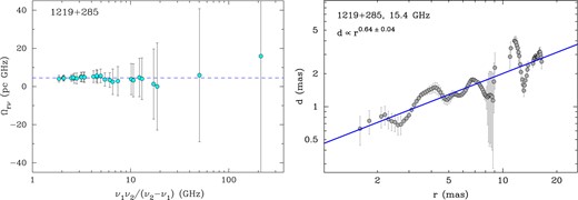
Left: Dependence of Ωrν on a frequency parameter ν1ν2/(ν2 − ν1) for BL Lacertae object 1219+285 constructed from VLBI observations at 1.4, 1.7, 2.3, 2.4, 4.6, 5.0, 8.1, 8.4, and 15.4 GHz. The dashed line denotes the median Ωrν. Smaller x-axis values correspond to wider frequency pairs and vice versa. Right: Evolution of the jet width as a function of the VLBI core separation at 15.4 GHz showing a quasi-parabolic streamline. The solid blue line represents the fitted dependence.
