


ABSTRACT
It has been claimed that the variability of field quasars resembles gravitational lensing by a large cosmological population of free-floating planets with mass |$\sim\!\! 10\ {\rm M}_{\oplus }$|. However, Galactic photometric monitoring experiments, on the other hand, exclude a large population of such planetary-mass gravitational lenses. These apparently contradictory pieces of evidence can be reconciled if the objects under consideration have a mean column density that lies between the critical column densities for gravitational lensing in these two contexts. Dark matter in that form is known to be weakly collisional, so a core develops in galaxy halo density profiles, and a preferred model has already been established. Here, we consider what such a model implies for Q2237+0305, which is the best-studied example of a quasar that is strongly lensed by an intervening galaxy. We construct microlensing magnification maps appropriate to the four macro-images of the quasar – all of which are seen through the bulge of the galaxy. Each of these maps exhibits a caustic network arising from the stars, plus many small, isolated caustics arising from the free-floating ‘planets’ in the lens galaxy. The ‘planets’ have little influence on the magnification histograms but a large effect on the statistics of the magnification gradients. We compare our predictions to the published Optical Gravitational Lensing Experiment (OGLE) photometry of Q2237+0305 and find that these data are consistent with the presence of the hypothetical ‘planets’. However, the evidence is relatively weak because the OGLE data set is not well suited to testing our predictions and requires low-pass filtering for this application. New data from a large, space-based telescope are desirable to address this issue.
1 INTRODUCTION
Dark matter, first inferred by Fritz Zwicky (Zwicky 2009, republication in English translation of the 1933 German original), has been the focus of a great deal of attention over the last few decades (Trimble 1987; de Swart, Bertone & van Dongen 2017). It appears to be the main form of matter in the Universe, but its fundamental nature is still unclear. Models of galaxy formation have demonstrated considerable success when the model universe starts out with dark matter predominantly in the form of non-relativistic elementary particles having no electromagnetic interaction (e.g. Davis et al. 1985; Peacock 1999). However, there has been no firm detection of a suitable elementary particle in the laboratory (e.g. Feng 2010; Boveia & Doglioni 2018). Although other forms of dark matter might lack such an attractive theoretical framework, one can nevertheless look for observational manifestations of any kind; and searches for the gravitational lensing signature of macroscopic lumps of dark matter have been informative, as follows.
Paczyński (1986) focused the attention of the astronomical community on the use of gravitational lensing to detect lumps of dark matter in the Galactic halo. The expected optical depth for this process is very small, so a large number of background stars must be monitored in order to make progress, but with a clear target to aim at several groups took up the challenge (Alcock et al. 1993; Aubourg et al. 1993; Udalski et al. 1993). Because of the short time-scales that go hand-in-hand with a small Einstein ring radius, a given optical depth leads to many more expected events if it resides in low-mass lumps. However, very few short-duration events were detected and a quasi-spherical Galactic dark halo consisting predominantly of planetary-mass compact objects is now ruled out (Alcock et al. 1998; Tisserand et al. 2007; Wyrzykowski et al. 2011; Griest, Cieplak & Lehner 2014). More recently, some short-duration microlensing events have been detected in photometric monitoring of Galactic bulge stars, and interpreted as free-floating planets (Sumi et al. 2011), but that population has been shown to be much smaller than first thought (Mróz et al. 2017; Sumi et al. 2023), and is dynamically insignificant. Constraints are also available for compact lenses in the planetary and sub-planetary mass range from high-cadence Subaru monitoring of M31 (DeRocco, Smyth & Profumo 2024).
The non-detection of planetary-mass lenses in the Galactic halo means that planetary-mass black holes are now an unattractive dark matter candidate. However, before the Galactic photometric monitoring experiments had delivered their results it had already been proposed by Hawkins (1993, 1996) that a large, cosmological population of planetary-mass black holes could be responsible for the optical variability that is observed in field quasars. Also, separately, Schild (1996) had argued for a large population of what he called ‘rogue planets’, on the basis of a possible microlensing signal in the macrolensed quasar Q0957+561. These claims were startling when they were first made, but neither one has been categorically refuted. There is, however, considerable ambiguity because of uncertainty about the size of quasar emission regions. If the source radius is as small as |$\sim\!\! 3\times 10^{14}\ {\rm cm}$|, then the low amplitude of any microlensing fluctuations in Q0957+561 excludes Schild’s rogue planets making up all of the dark matter in the lens galaxy, whereas they are allowed if the source is as large as |$\sim\!\! 3\times 10^{15}\ {\rm cm}$| (Wambsganss et al. 2000). Additional ambiguity arises from the unknown transverse velocities of the source and microlenses. For example, assuming stellar-mass microlenses and a source radius as large as |$\sim\!\! 4\times 10^{16}\ {\rm cm}$|, Schechter et al. (2003) attributed the rapid, low-amplitude microlensing fluctuations of the macrolensed quasar HE 1104−1805 to relativistic transverse motion of the source.
The scenario advocated by Hawkins (1993) was analysed by Schneider (1993), who used quasar photometry from Hawkins & Veron (1993) to limit the possible cosmological abundance of microlenses, as a function of lens mass – the point being that large flux excursions are observed to be very rare in practice, whereas massive lenses should sometimes introduce high magnifications. However, the Schneider (1993) study did also show that a large fraction of the cosmological critical density could be present in lenses of mass |$\lesssim\!\! 10^{-4}\ {\rm M_\odot }$| without generating any conflict with the observed quasar light curves. Zackrisson & Bergvall (2003) and Zackrisson et al. (2003) independently reassessed the lensing interpretation of field quasar variability, finding it to be viable1 when taken in isolation. Walker & Lewis (2003) investigated the effect of nanolenses on gamma-ray bursts but found that the available data could not significantly constrain their abundance.
As described above, the Galactic photometric monitoring experiments exclude the possibility that the Galactic dark matter resides in either planets or planetary-mass black holes; however, objects that have a peak column density |$\Sigma _0 \lesssim 10^5\,\,{\rm g\, cm^{-2}}$| do not automatically violate the Galactic constraints because they are not strong gravitational lenses in that context. Such objects do have a photometric signature when they occult Galactic stars, both from gas lensing (Draine 1998; Rafikov & Draine 2001) and dust extinction (Kerins, Binney & Silk 2002; Drake & Cook 2003). However, the form of the resulting light curves is at present unknown and consequently a population of this type is difficult to constrain: we do not know what signature to look for. Furthermore, there is a fundamental difficulty in using any type of optical occultation signal to constrain a population of dusty objects in the Galaxy, because dust extinction creates an anticorrelation between foreground clouds and detectable background stars.2
With those points in mind, Tuntsov & Walker (2022) revisited the possibility of a large cosmological population of planetary-mass lenses, giving attention specifically to objects that are weak gravitational lenses when placed in the Galaxy, but strong at cosmological distances. Although these characteristics are not known to correspond to any form of matter that has been directly observed, so it is debatable whether such objects exist at all in our Universe, it is worth mentioning that there are at least some theoretical counterparts in the structural models of H2 snow clouds presented by Walker & Wardle (2019).
For the larger column densities in the range studied by Tuntsov & Walker (2022), the magnification statistics for a given lens mass were found to be largely independent of Σ0. That result is easily understood: once the objects become very strong gravitational lenses, the dominant images form far from the centre (‘outside the cloud’), where the densities of gas and dust are too small to have a significant effect on the measured flux. In that regime, the constraints reported by Tuntsov & Walker (2022) parallel those previously reported by Schneider (1993), as indeed they should because the new simulations followed essentially the same approach as the original. In that respect, the main difference between the two works is the 3× larger source size adopted by Tuntsov & Walker (2022). However, Tuntsov & Walker (2022) also undertook simulations for lens masses lower than Schneider (1993) considered, and by doing so they were able to demonstrate that the mass range 10−4.5 ± 0.5 M⊙ is preferred, in the sense that the corresponding magnification statistics can quite closely resemble those of the Hawkins & Veron (1993) data.
Unfortunately, even a model that nicely reproduces the Hawkins & Veron (1993) data cannot be considered strong evidence regarding the nature of the dark matter, because we cannot be sure that field quasars really are varying primarily as a result of gravitational lensing rather than varying intrinsically. To address that issue, we need instead to examine the variability of quasars that are macrolensed – i.e. strongly lensed by a foreground galaxy. For such systems, any variations that are intrinsic to the source show up in all of the macro-images, whereas the lumpiness in the mass distribution within the lens galaxy leads to different microlensing variations for each of those images (Gott 1981). This paper therefore addresses the question of what behaviour is predicted for a macrolensed quasar when the dark matter in the lensing galaxy is made up predominantly of the type of objects preferred by Tuntsov & Walker (2022), and how those predictions compare to observations. For simplicity, in this paper we illustrate the expected nanolensing signals using a model in which all of the ‘missing mass’ inferred from dynamics is in the form of dense gas clouds, with no significant contribution from non-baryonic matter. As noted earlier, this sort of model is not preferred by cosmologists; nevertheless, it forms a clear limiting case from which useful insights can be obtained.
Many examples of macrolensed quasars are now known (e.g. Treu 2010). In this paper, we focus on just one system, Q2237+0305, in which the lens galaxy has an exceptionally low redshift (z = 0.0394; Huchra et al. 1985), making it well suited to our application (for reasons that are discussed later, in Section 6.2). Optical monitoring of Q2237+0305 has been undertaken by the Optical Gravitational Lensing Experiment (OGLE) team for more than a decade, and the resulting, high-quality data have been placed in the public domain (Woźniak et al. 2000; Udalski et al. 2006); we make use of those data in this paper. Many analyses of Q2237+0305 light curves have been undertaken previously (e.g. Kochanek 2004; Poindexter & Kochanek 2010), including work that gave attention to planetary-mass objects (Wyithe, Webster & Turner 2000b, who ruled out Jupiter-mass compact objects as a significant contribution to the mass of the bulge of the lens galaxy).
There are several motivations to revisit the constraints on planetary-mass lumps in Q2237+0305: first, we have a preferred mass range to focus on, so the model predictions are correspondingly specific; secondly, in the time since Wyithe et al. (2000b) was published the total duration of the OGLE light curves for Q2237+0305 has increased fivefold; thirdly, the properties of the stellar bulge of the lens galaxy are now accurately determined (van de Ven et al. 2010); and, finally, the planetary-mass objects under consideration here are much less compact than was assumed in previous analyses, with important implications for the lensing model. The point there is that dark haloes made up of low column density objects are weakly collisional and develop a core in their density profile (Walker 1999). Moreover, a preferred column density for the individual dark matter lumps has already been determined from consideration of their collisional properties (Walker 1999), and that in turn fixes a specific value for the central, nanolensing contribution to the optical depth of the lens galaxy – as described in Section 2.1.
The finite column density of the individual dark matter lumps also moderates the gravitational deflection angle, for light that passes through the lump itself; however, that is expected to have little influence on the magnification maps of Q2237+0305, for two reasons. First is that the preferred column of the individual lumps, |$\langle \Sigma \rangle \simeq 140\,\,{\rm g\, cm^{-2}}$| (see Section 2.1), is more than 60× larger than the critical surface density for strong gravitational lensing in Q2237+0305. In other words, the individual lumps are very much smaller than their own Einstein rings. Secondly, as discussed in Section 2.1, the central nanolensing optical depth of the lens galaxy is expected to be of the order of 0.1. Thus, the finite column density of the individual lumps makes no difference to 99.9 per cent of the rays (99.9 per cent of the area in the lens plane), and a point-mass approximation for the individual deflection angles is appropriate almost everywhere. Furthermore, the small fraction of rays for which the approximation is poor are themselves mostly not important, because they are typically strongly demagnified (‘overfocused’). We therefore employ the point-mass deflection angle approximation in our ray-shooting calculations in Section 3.
Because we are using the point-mass approximation for the deflection angle introduced by a planetary-mass lump, the results of the lensing calculations presented here are identical to what would be obtained if the same total mass were placed in planets rather than dense gas clouds. Consequently, for the remainder of this paper we will usually refer to the planetary-mass lumps as ‘planets’, with the inverted commas serving to remind readers that they are not actual planets.
This paper is structured as follows. In Section 2, we present our macro model of the Q2237+0305 lens, describing both the stellar component and the cored dark matter distribution. Then, in Section 3 we present our micro/nanolensing simulations. We undertake two distinct sets of calculations: one that includes both stars and the planetary-mass lumps of dark matter, and a comparison set that includes only stars; and we compare the statistical properties of the two distinct sets. Our comparison demonstrates that the rates of change of the image fluxes are potentially a powerful diagnostic for the presence of planetary-mass lumps of dark matter in the lens galaxy. In Section 4, we analyse the OGLE data for Q2237+0305 and then compare their statistical properties to those of the simulations in Section 5, finding a preference for the simulations that include the planetary-mass lumps of dark matter. In order to be able to make that comparison, it was necessary to first apply low-pass filtering to the OGLE data, and consequently we are unsure how strong our result really is. Section 6 discusses how that situation can be improved, arguing for daily observations with a large, space-based telescope. Our summary and conclusions are presented in Section 7.
2 MACRO MODEL OF THE Q2237+0305 LENS
Q2237+0305 is a well-studied quasar at a redshift of zs = 1.695, strongly lensed by a foreground spiral galaxy at zl = 0.0394 into a highly symmetric configuration of four images (a ‘quad’; Huchra et al. 1985). The four images are all seen through the stellar bulge of the lens galaxy, and they display strong independent brightness fluctuations due to microlensing (Irwin et al. 1989; Corrigan et al. 1991), superposed on flux variations that are common to all images.
A detailed study of the lensing galaxy was undertaken by van de Ven et al. (2010) who constructed axisymmetric dynamical models of the stellar bulge, constrained to match both the observed surface brightness profile and the kinematic profiles determined from integral field spectroscopy. Separately, van de Ven et al. (2010) also modelled the total mass distribution in the lens that is required to reproduce the observed image positions of the quasar. That total mass distribution proved to be consistent with the stellar mass distribution, so no dark matter is required to explain the macrolensing that is observed. Some dark matter may be present, but it is subdominant. Considering the uncertainties in the stellar mass-to-light ratio of the stars in the bulge, van de Ven et al. (2010) concluded that the dark matter fraction in the lens galaxy (if assumed to be constant) is constrained to be |$\lesssim\!\! 20$| per cent of the total.
In this paper, we adopt the isothermal lens model of van de Ven et al. (2010), for which the total convergence κt – i.e. surface density in units of the critical surface density for gravitational lensing, for this lens-and-source combination – of each image is as given in Table 1. The appropriate shear γ is equal to the total convergence, γ = κt in each case.
Total convergence values used for each of the four images of Q2237+0305. In our stars+‘planets’ microlensing simulations, the optical depth in |$10^{-4}\, \mathrm{M}_\odot$| point-mass lenses was set to κp = 0.043 for each of the images, with the remainder, κt − κp, comprised of |$0.1\, \mathrm{M}_\odot$| stars. For our ‘stars-only’ microlensing simulations, we set κp = 0.
| Image | A | B | C | D |
| Total κ = γ | 0.396 | 0.391 | 0.715 | 0.604 |
| Image | A | B | C | D |
| Total κ = γ | 0.396 | 0.391 | 0.715 | 0.604 |
2.1 The dark matter contribution
Models of galactic dynamics (e.g. Binney & Tremaine 2008) treat the constituent stars as point masses, because even over times as long as the age of the Universe physical collisions between stars are highly improbable. However, that is not true of the dark matter lumps under consideration in this paper, which have a much lower column density than stars. For example, our Sun has a mean column density |${M}_\odot /\pi {R}_\odot ^2\sim 10^{11}\,\,{\rm g\, cm^{-2}}$|, whereas, as described in the Section 1, we are considering gas clouds whose peak column density is |$\Sigma _0 \lesssim 10^5\,\,{\rm g\, cm^{-2}}$|. At low column densities, physical collisions between gas clouds limit their possible contribution to any virialized dark matter halo (Gerhard & Silk 1996).
That constraint was investigated by Walker (1999) who modelled the evolution of the density profile for a spherical dark matter halo comprised entirely of dense gas clouds (no non-baryonic dark matter) – a scenario consistent with the approach taken in this paper. Starting from a singular isothermal sphere, the evolved profile was found to be a cored isothermal sphere with the core radius depending on both the velocity dispersion of the halo and the mean column density of the individual clouds. Of course, material from the clouds that have undergone collisions simply becomes part of the pool of visible matter, so this model predicts a specific relationship between the circular speed of a dark halo and the total mass of visible material that should be present within it. Using published data, Walker (1999) demonstrated that the predicted, power-law relationship between visible mass and circular speed is obeyed by real galaxies, and that this provides a simple physical basis for the well-known Tully–Fisher relation for star-forming galaxies.3
The success of such a simple physical model gives support to the idea that dark haloes are indeed made up of dense gas clouds. However, for the purposes of this paper the key point is that by matching to data Walker (1999) was able to pin down the mean column density of the individual gas clouds: |$\langle \Sigma \rangle \equiv M/\pi R^2 \simeq 140\,\,{\rm g\, cm^{-2}}$|. And consequently the core radii of these collisional dark matter haloes can be predicted from their circular speeds alone. For the galaxy that is responsible for lensing Q2237+0305, the isothermal model of van de Ven et al. (2010) has a velocity dispersion of |$170\,\,{\rm km\, s^{-1}}$|, corresponding to a dark halo core radius of approximately 7.1 kpc (Walker 1999). That radius is several times larger than the projected separation of each of the four images from the centre of the lens galaxy, so the expected mean column density of the dark halo is approximately the same for all of them and approximately equal to the column at zero impact parameter. It is straightforward to integrate the density of a cored isothermal sphere along the line of sight, and expressing the result in terms of the critical surface density gives a central convergence (optical depth) of κp ≃ 0.043 in planetary-mass gas clouds.
The dark column just quoted is between 6 per cent and 11 per cent of the total columns given in Table 1 for the four images of Q2237+0305. Although van de Ven et al. (2010) did not formulate constraints for the particular case of a cored dark halo, their estimate of |$\lesssim\!\! 20$| per cent for a constant dark matter fraction is well above all our κp/κt values, so it is likely that our model could yield an acceptable fit to their data. In fact, the core radius of our model is sufficiently large that the dark halo surface density is almost constant in the region where the images of Q2237+0305 are formed, and consequently any lensing constraints are subject to the notorious mass-sheet degeneracy (see Schneider & Sluse 2013, for example). We also note that in our model the mean microlens mass is given by 〈mlens〉 ≃ (1 − κp/κt)〈m*〉, which is 89–94 per cent of the mean mass of the stars in the bulge, 〈m*〉. In other words, the mean microlens mass in our model is just that of a low-mass star, consistent with the findings of Wyithe et al. (2000b).
3 MICROLENSING SIMULATIONS
We generated two sets of magnification maps as a function of the source position using a bespoke ray tracing code, with the first putting all local mass density into stars only and the second allowing about 10 per cent of it to be in the substellar component. It is computationally challenging to use a large dynamic range in the mass of individual lenses and for this reason we used the top of the range of cloud masses preferred by Tuntsov & Walker (2022), |$M_\mathrm{ p}=10^{-4}\ \mathrm{M}_\odot$| as the ‘planet’ mass, and the mass of each of the stellar lenses was fixed at |$0.1\, \mathrm{M}_\odot$|; Appendix B discusses the effect of adopting a lower mass for the ‘planets’. Table 1 lists the lensing convergence (equal to the shear, for our isothermal macro model) for the four images of the quasar. For the stars+‘planets’ set, a value of κp = 0.043, the same for all images because of their highly symmetric configuration, is comprised of ‘planets’ and the rest is put into stars; for the star-only set, all of the convergence is in stars.
The resulting magnification maps are 2048 pixel × 2048 pixel squares, covering |$7.4\times 10^{17}\, \mathrm{cm}$| (four solar-mass Einstein radii, projected on to the source plane) on a side. This results in a resolution of ∼160 and ∼5 pixels per stellar and ‘planetary’ Einstein radius, respectively. The results are displayed in Figs 1 and 2 for one positive and one negative-parity image in the system – A and C, respectively; similar figures, Figs A1 and A2, for images B and D are included in the Appendix A. The maps are then convolved with the intensity distribution over the source profile, chosen as a disc with a Gaussian brightness profile of half-light radius |$R_S=3\times 10^{15}\, \mathrm{cm}$|, or approximately 8 pixels.
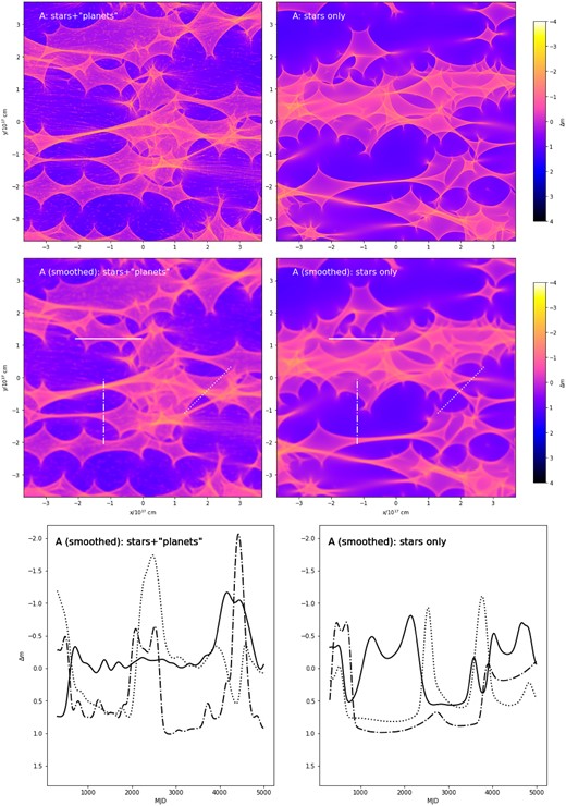
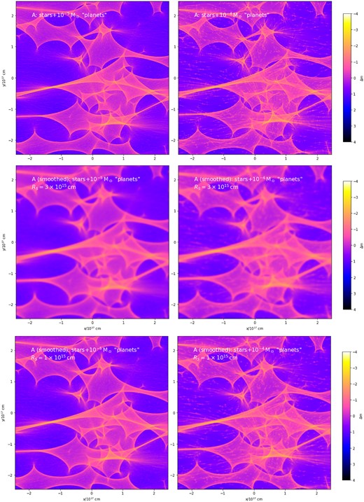
Microlensing magnification, in magnitudes, as a function of the source position for the positive-parity image A. The right column assumes that all mass is in stellar-mass objects, while the left includes a contribution from planetary-mass (nano)lenses. The top row is for a point (or, more precisely, pixel-sized) source, while the maps in the middle are convolved with a Gaussian disc of half-light radius |$R_s=3\times 10^{15}\, \mathrm{cm}$|. The bottom row provides examples of light curves for a source moving with an effective transverse velocity of |$5\times 10^3\, \mathrm{km}\, \mathrm{s}^{-1}$| along (solid curve), across (dot–dashed), and at 45° (dotted) to the large-scale shear stretching direction; the corresponding tracks are also marked in the middle row.
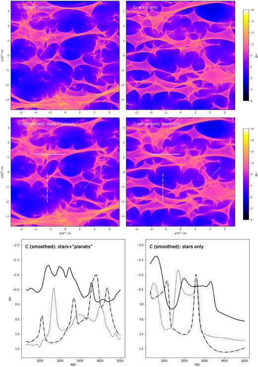
Same as Fig. 1 for image C, of negative parity.
As discussed in appendix A of Tuntsov & Walker (2022, see, particularly, their fig. A1), the information that is currently available in the literature favours quasar optical half-light radii in the range (1–5) × 1015 cm. Our chosen size for Q2237+0305 lies towards the upper end of that range, reflecting the fact that it is one of the more luminous quasars known. The photometric estimate for Q2237+0305 half-light radius along the lines of their appendix A returns values between 2.2 and |$4.8\times 10^{15}\, \mathrm{cm}$|, depending on the image chosen, and |$3\times 10^{15}\, \mathrm{cm}$| is a representative estimate. We discuss the effect of changing the assumed source size in Appendix B.
In order to convert magnification gradients into temporal derivatives in the image fluxes, we also need an estimate of the velocity at which the source moves relative to the magnification pattern. As discussed by Kochanek (2004), the observer contribution to the effective transverse velocity is inferred to be small, because Q2237+0305 lies not far from the axis of the observed dipole in the cosmic microwave background; and because the lens is at much lower redshift than the source the source contribution is also expected to be unimportant. With a distance ratio (source:lens) of approximately 11, a plausible value of around |$\sqrt{2}\times 300\,\,{\rm km\, s^{-1}}$| for the transverse velocity of the lens galaxy leads us to our adopted value for the source-plane projected transverse velocity of |$5000\,\,{\rm km\, s^{-1}}$|.
4 COMPARISON DATA AND FILTERING
The OGLE has been monitoring Q2237+0305 since 1997, resulting in a dense and homogeneous set of accurate photometric measurements for all four images of the system, spanning over a decade in time (Udalski et al. 2006). These data are available to the astronomical community in the OGLE Internet data archive,4 where we downloaded it from. The data contain magnitude measurements for the four images and their uncertainty estimates with, on average, one photometric point every few days, with some seasonal gaps. The photometric uncertainty ranges from under 10 mmag in the brightest image, A, to about 30 mmag for image D, which is 1–2 mag fainter.
These OGLE data, which are displayed in the top panel of Fig. 3, form our starting point for comparing the statistics of observed light-curve derivatives with the results of our microlensing simulations. There are, however, two issues that we need to face up to when making use of these data. One is the intrinsic variability of the source, which contributes to the observed light-curve derivatives for each of the images, and the other is photometric errors, which make estimates of the magnification derivatives noisy.
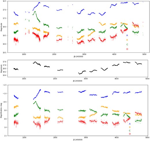
The top panel displays OGLE light curves for the images of Q2237+0305, shown with the original error bar estimates along with their smoothed versions, obtained by fitting harmonic series with periods above 60 d. The middle panel presents the mean of the four (smoothed) light curves, which we use as an estimate of the intrinsic variations in the source. The bottom panel shows the difference between the data at the top and middle panels, interpreted in this paper as an estimate of the microlensing magnification. We dropped seasons with only a handful of measurements (near MJD51100 and MJD52600) where low-pass filtering makes little sense.
The latter is important for us because even the best of the raw photometric sequences (image A) manifests photometric noise at the level of ∼10 mmag differences over spacings ∼3 d – corresponding to gradient noise |$\sim\!\! 3\,\,{\rm mmag\, d^{-1}}$| and, as we show later (Section 5, and in particular Fig. 4), the predicted signals also manifest at the level of |$\sim\!\! 3\,\,{\rm mmag\, d^{-1}}$|. To deal with the noise, we low-pass filter the individual light curves, fitting them with harmonic time series with periods limited from below. We chose a limit of 60 d, recognizing the scale of the structure we want to remain sensitive to and the data cadence, but the results are fairly insensitive to the smoothing scale choice.

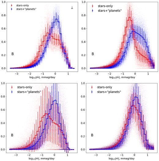
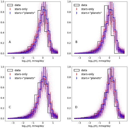
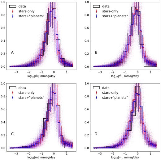
Histograms showing the distribution of the two components of the gradient of the (smoothed) magnification maps generated for each macro-image: A, B, C, and D, from top to bottom. The left-hand column shows the component parallel (∥) to the shear, and the right-hand column shows the perpendicular (⊥) component. Blue lines show the case with both stars and planetary-mass lenses; red lines show the case with stars only. In both cases, the histograms are averages over the whole map. A source velocity of |$5\times 10^3\, \mathrm{km}\, \mathrm{s}^{-1}$| is used to convert the gradient into time derivatives. The solid black line shows the observed distribution of light-curve derivative in smoothed OGLE data from Fig. 3 and the dashed line is for simulated light curves containing noise at the level reported by OGLE – processed in the same way as the actual data (note that the histograms are normalized).
To estimate the intrinsic variations, we simply form the average of the four low-pass filtered light curves. [Note that the time delays between the images are expected, and tentatively measured, to be small – of the order of hours (see Schmidt, Webster & Lewis 1998; Dai et al. 2003; Vakulik et al. 2006; Wertz & Surdej 2014).] The result, which is shown in the middle panel of Fig. 3, is inevitably contaminated by microlensing in the sense that it includes, at each epoch, the microlensing magnification averaged over all four images.
Subtracting our estimate of the intrinsic variations from the light curves of the individual images then provides us with our estimates of the microlensing signals for each of the four images separately, as shown in the lower panel of Fig. 3. These individual microlensing sequences are (to the extent that relative time delays are negligible) free of contamination by the intrinsic variations of the quasar. However, because our estimate of the intrinsic variations includes the mean of the microlensing magnifications, the individual microlensing sequences are themselves also contaminated by the (negative of) mean microlensing magnification. This framework for data analysis is new, so in Appendix C we repeat the statistical analysis of Section 5 using the more traditional approach (e.g. Esteban-Gutiérrez et al. 2023) involving magnitude differences between image pairs. That path leads to essentially identical conclusions.
5 LIGHT-CURVE STATISTICS
Figs 1 and 2 compare the microlensing magnification maps in the stars-only and stars+‘planets’ cases. Despite ‘planets’ only making about ∼10 per cent contribution to the optical depth, the effect of adding them is striking. The extended low-magnification ‘valleys’ and high-magnification ‘plateaus’ with a characteristic size of |$10^{16-17}\, \mathrm{cm}$|, corresponding to years-long time spans for realistic effective velocities, develop small-scale bumps, and, in the valleys for negative-parity images, dips of a characteristic shape. At a ‘planet’ mass of |$10^{-4}\, \mathrm{M}_\odot$| and parameters appropriate for Q2237+0305, their size is |$\sim\!\! 10^{15-16}\ \mathrm{cm}$|, right at the scale that is big enough to not be completely smoothed out by the finite source size effects, yet small enough to be probed with observations on |$\sim \,$|weekly time-scales.
We found the magnification distributions of the stars+‘planets’ and stars-only cases to be broadly similar. This is consistent with the expectation (Wambsganss 1992; Lewis & Irwin 1995; Wyithe & Turner 2001) for the magnification distribution to be only weakly sensitive to the microlens mass distribution (apart from the moderating effects of a finite source size). However, we note that Schechter, Wambsganss & Lewis (2004) demonstrated the situation to be significantly more complex, and the issue has not been resolved yet. It is clear though that the small-scale structure significantly affects the statistics of magnification derivatives, as can be seen in Fig. 4. This is particularly the case for the positive-parity images A and B, whose stars-only magnification maps contain extensive low-magnification valleys with very little small-scale structure – especially where source tracks happen to align with the direction along which the micro-caustic structure is stretched by the large-scale shear. The small-scale ‘planetary’ structure disturbs such quiet regions, in the process making the derivative statistics somewhat less anisotropic. Derivatives both along and across the large-scale stretching direction are enhanced, though the contrast is greater for the former.
The large effect of ‘planets’ on the distribution of magnitude derivatives suggests using that statistic to assess which of the two scenarios matches best to the OGLE data. In practice, we can only measure the derivative along the particular direction in which the image tracks through the magnification map – i.e. a linear combination of the two components of the gradient. The orientations of the actual tracks in the images of Q2237+0305, and thus the relative contributions of the two components, are not well constrained (Wyithe, Webster & Turner 1999; Tuntsov, Walker & Lewis 2004; Poindexter & Kochanek 2010); and the random motion of the microlenses in the bulge of the lens galaxy is also expected to contribute significantly to the time derivative (Wyithe, Webster & Turner 2000a). However, the change in shape of the histograms that is effected by the introduction of ‘planets’ is qualitatively similar for both components of the magnification gradient, which encourages a comparison with the data even in the absence of a unique value for the transverse velocity. Intriguingly, the observed distributions shown in Fig. 4 as black curves do look more like the blue, stars+‘planets’ and less like the red, stars-only histograms. Bearing in mind that only the horizontal position and not the shape of the simulated histogram depends on the unknown velocity, the observed narrower distributions and their sense of asymmetry appear consistent with the presence of ‘planets’, particularly for the A and B images, in which the difference between the two cases is most pronounced.
However, at present the preference for the stars+‘planets’ case is not much more than suggestive. Although the predicted derivative distributions for our entire simulated magnification maps are clearly distinct, there is substantial variation in these distributions among the various possible realizations of individual tracks within the maps. This is illustrated in the upper left panel of Fig. 5, which plots the vertical derivative distributions for 2048 individual columns of the maps for image B, shown in the middle panels of Fig. A1 – a case that, from Fig. 4, appears most favourable for distinguishing between the two cases. Even for these light curves, which are ideally matched to the extent and resolution of the magnification maps, the scatter is so large that it seems challenging to attribute any particular distribution to either red or blue set. Subsequent panels of the figure add, cumulatively, the effects of the unknown track orientation (upper right), OGLE-like sampling (bottom left), and OGLE-like noise (bottom right – these light curves are low-pass filtered before the derivatives are estimated). Finally, Fig. 6 compounds the above effects by forming and subtracting the estimate of the intrinsic light curve (inevitably contaminated by the microlensing) for each simulated set of four light curves, and computes their derivative distribution; the statistics of the resulting histograms are compared to the observed derivative distribution for all images.
Degradation of the attribution capacity of the magnification derivative histograms with practical constraints. The top left panel shows the average (as a step line plot) and standard variation (as error bars) of the magnification distributions among a set of 2048 light curves covering the full magnification maps along its columns; scattered points, shifted randomly within each bin for visual clarity, represent individual histograms. The top right panel accounts for the unknown orientation of tracks and the bottom left panel mimics the sampling pattern of the actual OGLE data set. The bottom right panel displays the effect of adding to the simulated magnification of a Gaussian noise with the amplitude reported by OGLE as their photometry estimated accuracy; for noisy data, the derivatives are computed after low-pass filtering them in the same way as done for the actual OGLE light curves. Note the effect of noise on the average of the statistic.
Predicted distribution, and its variation, for the magnification derivative in the low-pass filtered simulated noisy light curves from which an estimate of the intrinsic variation in each set of four light curves has been subtracted. The black lines show the derivative distribution of the actual light curves processed in the same way.
The progressive degradation seen in the panels of Fig. 5 suggests that it is mostly the noise that deprives the magnification derivatives of their power to discriminate between the stars-only and stars+‘planets’ cases. Moreover, unlike poor sampling, which only increases the expected variation in the statistic without affecting the mean value much, the addition of (as assumed here, white) noise distorts the latter, which diminishes prospects to improve the discriminating power with better sampling. This suggests that it might not be possible to rule out (or in) a subdominant low-mass lens population using only the available data. On the flip side, reducing the measurement noise would be on the top of the wish list for a future data set that would allow a definite test for the presence of nanolenses in Q2237+0305, followed by improved sampling. Encouragingly, this is also the conclusion of a study (Lewis et al., in preparation) using machine learning algorithms and human classifiers to distinguish between simulated stars-only and stars+‘planets’ cases. Relying on light-curve features that are not fully captured in the statistics that this paper focuses on, the algorithms are able to outperform the human classifiers in terms of false (‘planet’) positives if the noise is sufficiently reduced.
6 DISCUSSION
6.1 X-ray line shifts in lensed quasars
A substantial population of free-floating planetary-mass objects has previously been suggested to exist in external galaxies (Dai & Guerras 2018; Bhatiani, Dai & Guerras 2019), based on time-varying shifts in the Fe Kα line energy that were observed for several gravitationally lensed quasars (Chartas et al. 2017). Those studies are qualitatively consistent with the picture advanced in this work, but quantitatively they are inconsistent because Dai & Guerras (2018) and Bhatiani et al. (2019) estimated the population to be much smaller, and dynamically unimportant. However, those estimates rely on a specific model for the quasar’s X-ray line emission – intensity as a function of both spatial and velocity coordinates – and at present our knowledge of that intensity structure is not reliable.
6.2 Other multiply imaged quasars
In this paper, we have concentrated our attention on just one multiply imaged quasar, Q2237+0305. However, many strongly lensed quasars are known (e.g. Treu 2010; Agnello et al. 2018; Lemon et al. 2023), and dozens of those now have high-quality light curves available, which raises the question of whether there are any other systems that might be useful in searching for a planetary-mass population in the lens galaxy? Ultimately, that question must be answered on a case-by-case basis; however, the general outlook can be readily summarized: Q2237+0305 is particularly well suited to our purposes because of the exceptionally low redshift of the lens galaxy. There are two main considerations. First, for planetary-mass lenses the predicted amplitude of the photometric signal is quite modest even for Q2237+0305, and for more distant lens galaxies the amplitude decreases because the size of the magnification structure goes down relative to the size of the source. Secondly, the very low redshift of the lens in Q2237+0305 means that its contribution to the (source plane) effective velocity is expected to be very large – as discussed by Kochanek (2004) – and the nanolensing event rate is expected to be correspondingly high. Thus, for Q2237+0305 the nanolensing events are expected to be bigger and more frequent than for a typical lensed quasar. Moreover, these differences are substantial, because a typical lens – e.g. in the sample studied in the COSMOGRAIL (COSmological MOnitoring of GRAvItational Lenses) project (Millon et al. 2020) – has a redshift that is an order of magnitude greater than in Q2237+0305.
All this is not to say that Q2237+0305 is the best possible system for this type of study, as there is no fundamental barrier to the existence of a quasar that is lensed by an even closer galaxy (and with a greater transverse velocity, and a smaller source, etc.). New, deeper surveys for lensed quasars have the potential to discover a system that is superior to Q2237+0305 in these respects.
6.3 A call for new data on Q2237+0305
The influence of planetary-mass lenses can be clearly seen in our simulations – in the magnification maps, the simulated light curves, and the histograms of magnification gradients – but that is in part because the calculations are very precise. In fact, each nanolens produces only a small-amplitude photometric signal, comparable to the error bars on the OGLE data – hence the need for smoothing, and motivating our application of low-pass filtering to the data. Although low-pass filtering is a legitimate procedure to use, it does create some concerns. First, it means that the models are being compared with a signal that is one step removed from the measurements themselves. Secondly, it is possible that the smoothed data might be limited by low-level systematic errors – associated with, for example, lunation or variations in atmospheric transparency – that can masquerade as a microlensing signal. Consequently, we cannot gauge the level of support for the model of dark matter in the form of planetary-mass gas clouds given by the currently available OGLE data.
The problems just mentioned can be addressed by obtaining a new data set. With a large telescope, and exposure times of only a few minutes, the photon noise limit can be better than 1 mmag, even for the faintest of the four macro-images of Q2237+0305. And because the requisite exposure times are short such observations can be undertaken with a high cadence (e.g. daily) for the whole observing season. In that way, one can ensure that if the predicted nanolensing fluctuations are manifested in the light curves, then they would be well sampled by the observations and would be measured with high signal-to-noise ratio.
Although high signal-to-noise ratio and high cadence are both important, they are not sufficient to guarantee a clear detection of the predicted signal (or tight limits on the absence thereof) in Q2237+0305: it is also essential to ensure that systematic errors – in particular, fluctuating systematic errors – are reduced to a level where they are insignificant. That is difficult to achieve at high levels of precision because of, for example, low-level residual variations in the sky background, the atmospheric transparency, and the point spread function. However, by far the largest contributions to those effects come from the Earth’s atmosphere, and if we observe from space it is possible to keep systematic errors to a level well below 1 mmag. In the near future, the large-aperture space telescopes that will permit targeted observations include JWST (McElwain et al. 2023) and the Nancy Grace Roman space telescope (formerly Wide-Field InfraRed Survey Telescope, WFIRST; Akeson et al. 2019); but both of these are primarily infrared telescopes, which is not ideal for quasar microlensing studies because the size of the emission region increases with wavelength. The Hubble Space Telescope (Williams 2020), on the other hand, has a large aperture and can observe in the visual, blue, or even ultraviolet bands – it appears to be the best of the available space telescopes for this task.
7 SUMMARY AND CONCLUSIONS
Planetary-mass gas clouds are able to explain the statistically symmetric and largely achromatic variability of field quasars if they make a significant contribution to the dark matter budget, while nevertheless evading Galactic constraints on compact low-mass lenses (Tuntsov & Walker 2022). A population of such clouds would form cored baryonic dark matter profiles in the galactic context and, at the characteristic cloud column density implied by the observed properties of star-forming galaxies (Walker 1999), the clouds remain strong lenses when placed outside of the Local Group, at z ≳ 0.01.
In this paper, we considered the effect of such planetary-mass nanolenses on the light curves of Q2237+0305 – one of the best-studied, multiply imaged quasars (Huchra et al. 1985). The four images of this quasar are seen through the bulge of a much nearer lens galaxy and display prominent microlensing signals (Irwin et al. 1989), which can be separated from any intrinsic variation in the background quasar source because the time delays between images are all very small. The macrolensing model is tightly constrained by the observed image astrometry, surface photometry, and integral field spectrometry of the lens galaxy (van de Ven et al. 2010). Also, a long, homogeneous photometric record of the four images has been accumulated by the OGLE project (Udalski et al. 2006).
The nanolensing population is predicted to remain a subdominant mass component, providing about 10 per cent of the total lensing convergence, the rest contributed by the stellar population of the bulge. We simulated magnification maps appropriate to the projected location of the four images in the bulge and compared the predicted light curves to the available OGLE data. The nanolenses do not change the distribution of the microlensing magnification in any dramatic way, but the magnification derivatives are strongly affected. At face value, the observed distributions in Fig. 4 do look more like the simulations containing nanolenses than those with stellar-mass microlenses only. However, we do not believe this evidence to be conclusive for two main reasons. One is that the variation in the predicted derivative distribution from one realization to another is substantial due to the limited time sampling of the available data. The second is the inevitable noise in the available photometry, which both necessitates low-pass filtering of the data, to infer magnification derivatives, and biases the model predictions (cf. Fig. 5). We therefore conclude that, although the OGLE data are consistent with the presence of a significant population of nanolenses in the bulge of the Q2237+0305 lens galaxy, we cannot categorically decide the matter at present.
The photometric noise thus emerges as a primary observational challenge to the attempted test and we call for a highly accurate set of light curves from a larger, preferably space-based telescope to resolve the issue. The images are sufficiently bright for the |$\mathcal {O}(\mathrm{mmag})$| accuracy to be achieved with reasonable demand on the exposure time. We are also exploring alternative data characterization methods designed to better handle the information not captured by the magnitude derivative statistics, such as machine learning classification.
ACKNOWLEDGEMENTS
GFL received no financial support for this research. We thank the referee for thoughtful suggestions.
DATA AVAILABILITY
The data underlying this article will be shared on reasonable request to the corresponding author.
Footnotes
Although, they argued, not the whole story: low-redshift active galactic nuclei vary intrinsically, so presumably quasars do also at some level.
Thus, motivating work at longer wavelengths where the extinction is negligible (Suvorov et al., in preparation).
It is now widely accepted that a relationship between visible mass and halo circular speed does indeed underlie the Tully–Fisher relation; it has since become known as the ‘Baryonic Tully–Fisher Relation’ (following McGaugh et al. 2000).
References
APPENDIX A: MAGNIFICATION MAPS FOR IMAGES B AND D
Figs A1 and A2 present magnification maps and example light curves for images B and D; they are qualitatively similar to Figs 1 and 2.
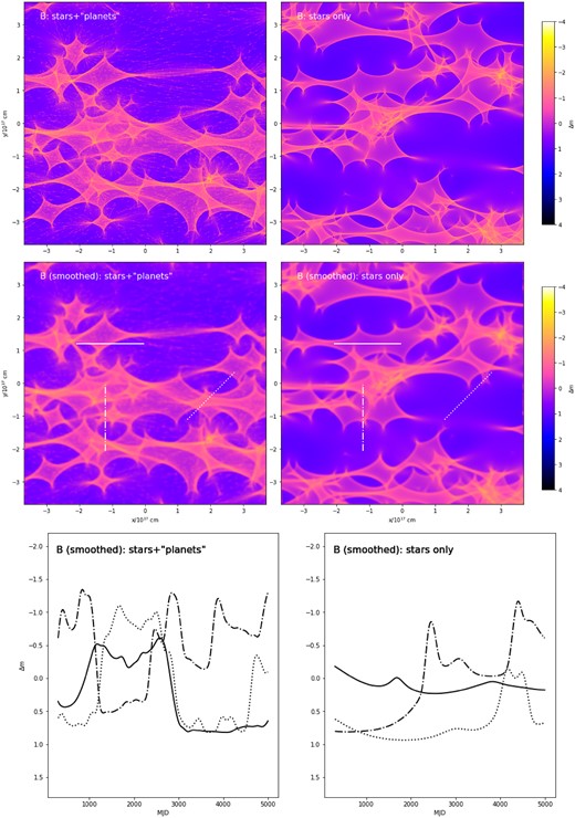
Same as Fig. 1 for image B, of positive parity.
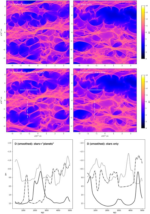
Same as Fig. 1 for image D, of negative parity.
APPENDIX B: RELAXING SOURCE SIZE AND LENS MASS ASSUMPTIONS
The nominal source half-light radius of |$3\times 10^{15}\, \mathrm{cm}$| chosen in this paper for Q2237+0305 is just over the Einstein radius of the planetary-mass lenses but is well below the Einstein scale of our stellar-mass lenses, which reflects in the effect this smoothing has on the structures induced by two classes of lenses in Figs 1, A1, 2, and A2. However, both types of structures induce the same (formally infinite) range of magnitude derivatives, and the effect of smoothing on the latter is not trivial. Fig. B1 shows how the statistics of light-curve derivatives (for a representative image and track orientation) change as the source size is varied by half an order of magnitude either side of its fiducial value, the range likely exceeding the reasonable uncertainty of this estimate in the optical band. Smoothing clearly suppresses the derivative due to both stellar and planetary-mass lenses, but to a different extent, with a |$10^{16}\, \mathrm{cm}$|-wide source big enough to totally erase the nanolensing signal.
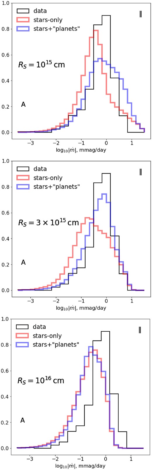
An extended source suppresses the variations due to both stellar- and planetary-mass magnifications, as summarized in Fig. 4-like histograms for derivatives along the large-scale shear stretching directions of image A. In particular, a half-light radius of just |$R_S=10^{16}\, \mathrm{cm}$| totally desensitizes this statistic to planetary-mass lenses in the Q2237+0305 case.
However, the source size effect is clearly subdominant to those of noise or irregular sampling, as revealed by Figs B2 and B3, showing analogues of Fig. 6 for smaller and larger sources. Even in the case of the smallest source size that least suppresses the ‘planetary’ signal, the limitations of the currently best available data (discussed in Section 5) make it difficult to distinguish between the presence or absence of low-mass lenses. This reinforces the case for a better data set, as presented in Section 6.3.

From the discussion in this section, one can also anticipate the effect of changing the nanolens mass to a smaller value. Reducing it to |$10^{-5}\, \mathrm{M}_\odot$| would shrink the Einstein radius by half an order of magnitude, and so, at a constant mass density, would change the typical separation between the lenses. One would therefore expect that even a smaller source size of |$\sim\!\! 10^{15}\, \mathrm{cm}$| would be quite detrimental to the discriminatory power of the light-curve derivative statistics, while the nanolensing signal would be strongly suppressed in the case of a half-light radius |$R_S=3\times 10^{15}\, \mathrm{cm}$| implied by the observed brightness of Q2237+0305.
Figs B4 and B5 illustrate those points. They present the magnification maps and their convolution with a Gaussian source of varying size assuming nanolenses of different masses for two representative images of positive and negative parity (we kept the positions of the stellar-mass lenses the same here). The magnification maps for these simulations were generated with the Fast Multipole Method-based algorithm of Jiménez-Vicente & Mediavilla (2022), as the computational resources used for our simulations in Figs 1–A2 were no longer available. In order to properly resolve the Einstein radius of the lower mass lenses in this simulation, we had to decrease the pixel size – which, given the limitation of the public interface5 to the Jiménez-Vicente & Mediavilla (2022) software, necessitated simulating a slightly narrower field of view, of approximately |$2.66\times 10^{17}\, \mathrm{cm}$| on a side. We checked that the two codes agreed on the output when the resolution, field of view, and the input positions and masses of the lenses were identical. The finer scale structure due to lower mass nanolenses is severely degraded by smoothing with our fiducial source of half-light radius |$R_S=3\times 10^{15}\, \mathrm{cm}$| and the degradation is still strong even for |$R_S=10^{15}\, \mathrm{cm}$|.
Comparison of the effect of nanolenses of a lower mass, |$10^{-5}\, \mathrm{M}_\odot$| (left), to that of our fiducial |$10^{-4}\, \mathrm{M}_\odot$| ‘planets’ (right) for image A. The top row shows the original magnification maps, while the middle and bottom rows convolve them with a source of half-light radius |$R_S=3\times 10^{15}\, \mathrm{cm}$| and |$R_S=10^{15}\, \mathrm{cm}$|.
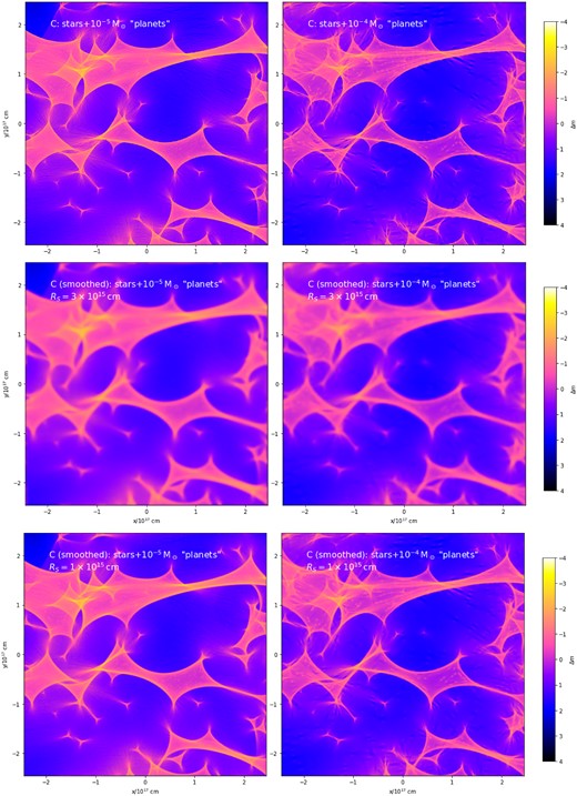
Same as Fig. B4 for image C.
Given this suppression, it is of little surprise that the light-curve derivative statistics expected for lower mass lenses do not separate as well from the ‘stars-only’ case, further reducing the sensitivity to ‘planets’ with the available data. Encouragingly though, with better sampling and increased accuracy, as advocated in Section 6.3, the statistics would be able to not only identify the presence of ‘planets’ but also gauge their mass, as Fig. B6 demonstrates in the case of a small source size. Only an indication of the presence of nanolenses but not a determination of their mass would be possible for a more realistic value of RS. The foregoing analysis suggests that even this quasar, which is particularly well suited for the detection of low-mass microlenses by virtue of a very low lens–galaxy redshift, would be insensitive to the presence of still lower mass microlenses, for any reasonable estimate of the optical source size.
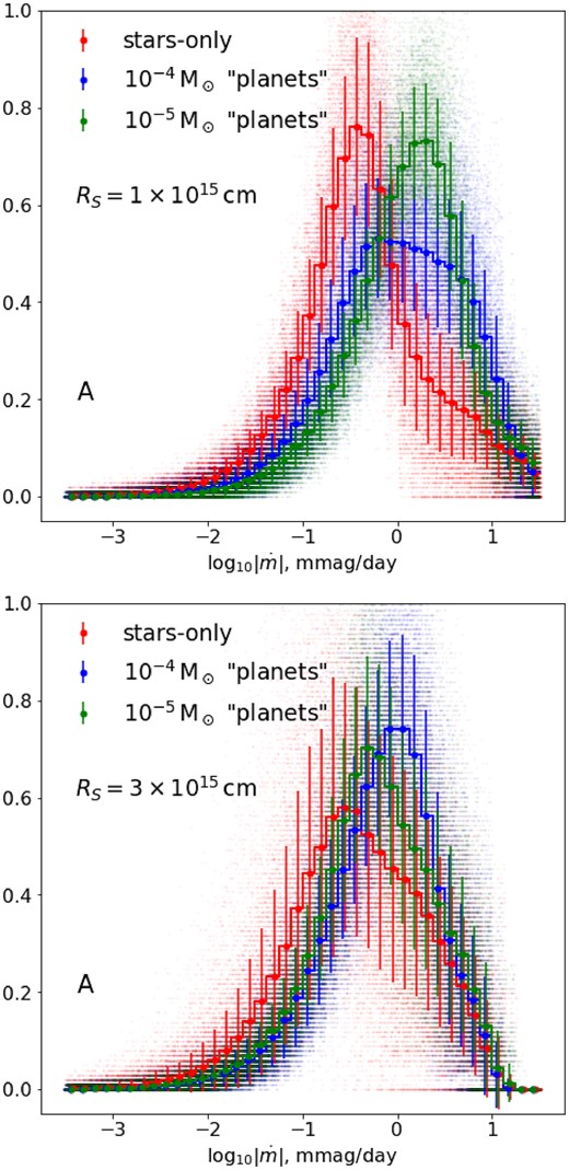
Distribution of light-curve derivatives for image A for different (if any) nanolens populations assuming a hypothetical data set with weekly cadence and negligible noise. The top figure shows that in the case of a small source, |$R_S=10^{15}\, \mathrm{cm}$|, the statistics would even be sensitive to the mass of the ‘planets’, although the bottom panel suggests that it would be difficult to go beyond establishing their very presence for a more realistic source size.
APPENDIX C: MAGNITUDE DIFFERENCE STATISTICS
To avoid having to form an estimate of the intrinsic variations of the source, it is possible to construct pairwise magnitude differences, which automatically removes intrinsic variations when the time delay between images is negligible. Indeed, that approach will be familiar to many readers and is a useful point of reference. We have therefore repeated our statistical analysis, but using pairwise magnitude differences, to see whether the data are better matched by simulated light curves with or without the planetary-mass microlens population. The results, in the familiar form of magnitude (difference) derivative histograms, mimicking Fig. 6 are shown in Fig. C1. Unfortunately, none of the image pairs appears able to discriminate between the two hypotheses.
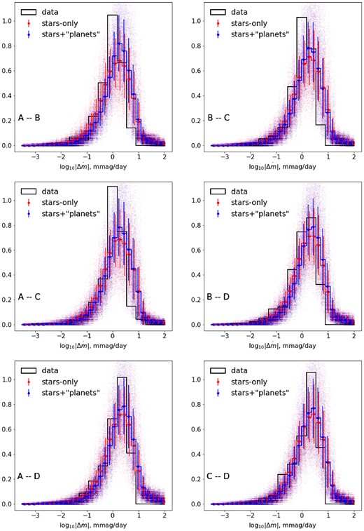
Histograms of the (smoothed) difference light-curve derivatives observed in all pairs of Q2237+0305 images compared to simulated light curves computed for magnification maps with and without planetary-mass microlenses, similar to that shown in Fig. 6.
