


ABSTRACT
We implement general relativistic hydrodynamics in the moving-mesh code arepo. We also couple a solver for the Einstein field equations employing the conformal flatness approximation. The implementation is validated by evolving isolated static neutron stars using a fixed metric or a dynamical space–time. In both tests, the frequencies of the radial oscillation mode match those of independent calculations. We run the first moving-mesh simulation of a neutron star merger. The simulation includes a scheme to adaptively refine or derefine cells and thereby adjusting the local resolution dynamically. The general dynamics are in agreement with independent smoothed particle hydrodynamics and static-mesh simulations of neutron star mergers. Coarsely comparing, we find that dynamical features like the post-merger double-core structure or the quasi-radial oscillation mode persist on longer time scales, possibly reflecting a low numerical diffusivity of our method. Similarly, the post-merger gravitational wave emission shows the same features as observed in simulations with other codes. In particular, the main frequency of the post-merger phase is found to be in good agreement with independent results for the same binary system, while, in comparison, the amplitude of the post-merger gravitational wave signal falls off slower, i.e. the post-merger oscillations are less damped. The successful implementation of general relativistic hydrodynamics in the moving-mesh arepo code, including a dynamical space–time evolution, provides a fundamentally new tool to simulate general relativistic problems in astrophysics.
1 INTRODUCTION
Numerical simulations are an important tool to study astrophysical systems involving compact objects such as core-collapse supernovae and binary mergers (Faber & Rasio 2012; Janka 2012; Rosswog 2015b; Baiotti & Rezzolla 2017; Foglizzo 2017; Janka 2017; Kotake & Kuroda 2017; Martínez-Pinedo et al. 2017; Roberts & Reddy 2017; Baiotti 2019; Bauswein & Stergioulas 2019; Duez & Zlochower 2019; Shibata & Hotokezaka 2019; Bernuzzi 2020; Radice, Bernuzzi & Perego 2020; Dietrich, Hinderer & Samajdar 2021; Janka & Bauswein 2022). The interpretation of the observations and the extraction of physics from such astronomical measurements to a large extent rely on numerical modelling of these events. For instance, observing binary neutron star (BNS) mergers provides the opportunity to study properties of high-density matter and the formation of heavy elements among several other fascinating aspects like short gamma-ray bursts. The recent simultaneous measurement of the inspiral stage of the BNS merger GW170817 and its electromagnetic counterparts (Villar et al. 2017; Abbott et al. 2017a, b), and especially the conclusions drawn from it, highlight the importance of numerical studies of these systems. Simulating compact objects can be challenging because many scenarios require the concurrent resolution of disparate length and time-scales of a highly dynamical system in three dimensions and the inclusion of various physical effects.
The bulk dynamics of such systems is governed by relativistic hydrodynamics in combination with a dynamical space–time. There exist several approaches to numerically treat relativistic hydrodynamics: most prominent are Eulerian grid-based methods (including finite-difference, finite-volume, or discontinuous Galerkin schemes) and Lagrangian smoothed particle hydrodynamics (SPH; for reviews see e.g. Wilson & Mathews 2003; Alcubierre 2008; Font 2008; Baumgarte & Shapiro 2010; Rezzolla & Zanotti 2013; Martí & Müller 2015; Shibata 2015; Rosswog 2015a, and references therein). Font (2008), Baiotti & Rezzolla (2017), and Foucart et al. (2022) provide a survey of codes currently used to tackle general relativistic hydrodynamic (GRHD) problems mostly in the context of binary mergers; some recent relativistic SPH tools are presented in Liptai & Price (2019) (adopting a fixed metric) and in Rosswog & Diener (2021) and Diener, Rosswog & Torsello (2022) (including a dynamical evolution of the space–time and applications to neutron star mergers).
Both Eulerian grid-based methods and SPH have specific advantages and limitations (see the above references for more detailed discussions). Eulerian methods solve the GRHD equations on a static mesh, where many modern codes include (adaptive) mesh refinement techniques to resolve specific regions of interest. These methods accurately resolve shocks and fluid instabilities through the implementation of high-resolution shock-capturing methods. However, they may suffer from grid effects, require a special treatment of vacuum regions, and, in the case of compact object mergers, following small amounts of high-velocity ejecta at large distances can be challenging.
SPH solves the Lagrangian hydrodynamic equations (comoving with the fluid) on particles representing a certain amount of rest mass. Advection and rest mass conservation are treated with high accuracy and the scheme offers an inherently adaptive resolution. Vacuum regions do not require a special treatment and tracer particles for nucleosynthesis calculations are trivially implemented. Traditionally, SPH is considered to resolve shocks and fluid instabilities poorer compared to high-resolution shock-capturing methods (but see e.g. Rosswog 2015a, and references therein for more modern techniques showing significant improvements). Notably, the Einstein equations cannot be solved in a particle-based discretization and thus require the inclusion of an additional computational grid and corresponding communication between both computational structures (similar problems may arise for treating other non-zero fields in the vacuum like magnetic fields).
Springel (2010) introduced the moving-mesh code arepo, which combines some of the advantages of Lagrangian SPH and Eulerian mesh-based hydrodynamics. arepo solves Newtonian hydrodynamics with a finite-volume approach on a moving unstructured mesh, which is constructed based on a set of mesh-generating points. The moving-mesh approach retains many of the advantages of mesh-based methods, while the mesh-generating points can move in an arbitrary way (see Springel 2010, for more details). Over the last years, Arepo has been employed for a wide range of astrophysical problems in cosmology, Type Ia supernovae, the common envelope phase in binary stars and various other systems (see e.g. Pakmor et al. 2013; Vogelsberger et al. 2014; Ohlmann et al. 2016; Weinberger et al. 2017; Koudmani et al. 2019; Schneider et al. 2019; Gronow et al. 2021; Pakmor et al. 2022). A number of other moving-mesh codes have subsequently been developed and applied to various astrophysical problems (Duffell & MacFadyen 2011, 2012; Gaburov, Johansen & Levin 2012; Duffell & MacFadyen 2013; Yalinewich, Steinberg & Sari 2015; Vandenbroucke & De Rijcke 2016; Chang, Wadsley & Quinn 2017; Ayache, van Eerten & Eardley 2022) with several works investigating high-order schemes on moving meshes (see e.g. Dumbser, Uuriintsetseg & Zanotti 2013; Dumbser et al. 2017; Gaburro et al. 2020, and references therein). All these applications have generally shown the usefulness and benefits of the moving-mesh approach as compared to more traditional schemes.
Moving-mesh codes can follow the fluid motion and allow to flexibly place resolution in physically interesting regions. Hence, they offer adaptive resolution, which follows the matter motion including the possibility to split or merge cells and by this to adaptively increase or decrease the resolving power. The quasi-Lagrangian nature of the scheme reduces numerical advection errors. These elements make moving-mesh codes particularly interesting for simulating compact objects and in particular BNS systems. In recent years, some moving-mesh codes have been extended to include GRHD (Ryan & MacFadyen 2017; Chang & Etienne 2020). However, all these implementations currently employ a fixed space–time, and to date no moving-mesh code evolves the space–time dynamically, as it would for instance be required to simulate neutron star mergers.
In this work, we extend arepo to simulate general relativistic systems (based on the upgraded implementation described in Pakmor et al. 2016). We implement GRHD into the code employing the Valencia formulation (Banyuls et al. 1997) and couple to it a solver for a dynamical space–time. The Einstein equations are solved on an independent overlaid grid adopting the conformal flatness approximation (Isenberg & Nester 1980; Wilson, Mathews & Marronetti 1996). We also include some additional modules to simulate neutron stars such as a high-density equation of state (EOS). We demonstrate the performance of the code in relativistic shock tube and blast wave problems. We further validate our implementation by computing equilibrium models of isolated neutron stars, which are benchmarked by comparing pulsation frequencies to perturbative results and other codes. Finally, we perform the first moving-mesh simulation of a BNS merger. We evolve the system for almost 40 ms into the post-merger phase and discuss the dynamical properties of the remnant and the characteristics of the GW signal.
The paper is structured as follows. Section 2 introduces the theoretical framework of our work. In Section 3, we provide details of our numerical implementation focusing on modifications with respect to the original code (Springel 2010; Pakmor et al. 2016). In Section 4, we present simulations of isolated, static stars. In Section 5, we describe the initial data for BNSs and present a BNS merger simulation. In the last section, we provide a summary of our work and outline future plans. We also include appendices where we provide additional details on the theoretical formulation (Appendix A), present relativistic shock tube (Appendix B) and blast waves tests (Appendix C), and investigate certain aspects of the numerical treatment with additional isolated neutron star and BNS merger simulations (Appendix D). Throughout this work we set c = G = 1, unless otherwise specified. Greek indices denote space–time components, while Latin indices refer to spatial components.
2 THEORETICAL FORMULATION
We briefly present the basic equations implemented in the relativistic version of arepo.
2.1 Field equations
We adopt the ADM formalism (Arnowitt, Deser & Misner 2008) to foliate the space–time into a set of non-intersecting space-like hypersurfaces with a constant coordinate time t. The general metric element then reads
where gμν is the space–time 4-metric, α denotes the lapse function, βi is the shift vector, and γij the spatial 3-metric.
In this work, we impose the conformal flatness condition (Isenberg & Nester 1980; Wilson, Mathews & Marronetti 1996), which approximates the spatial part of the metric as
where ψ is the conformal factor and |$\hat{\gamma }_{ij}$| is the flat metric, i.e. |$\hat{\gamma }_{ij}=\delta _{ij}$| in Cartesian isotropic coordinates, which we use in our treatment.
Adopting the maximal slicing condition Tr(Kij) = 0, where Kij is the extrinsic curvature, the Einstein equations reduce to a set of five coupled non-linear elliptic differential equations and read
where E, S, and Si are matter sources terms. We adopt the energy–momentum tensor of a perfect fluid, namely
where ρ is the rest-mass density, h = 1 + ϵ + p/ρ is the specific enthalpy, ϵ is the specific internal energy, p is the pressure, and uμ is the 4-velocity of the fluid. Then, in the system of differential equations (3)–(5), the various matter contributions in the source terms are given by
Within the conformal flatness approximation, the extrinsic curvature follows directly from the metric elements as
Following Baumgarte et al. (1998), we introduce the definition |$\beta ^i=B^i-\frac{1}{4}\partial _i\chi$|. Then equation (5) can be rewritten as two Poisson-like differential equations for the two auxiliary fields Bi and χ, which read
and can be solved iteratively.
For more details about the numerical implementation see Section 3.7 and Oechslin, Rosswog & Thielemann (2002) and Oechslin, Janka & Marek (2007).
2.2 General relativistic hydrodynamics
The equations of GRHD result from the conservation laws for the energy–momentum tensor Tμν and matter current density Jμ = ρuμ. By choosing a set of appropriate conserved variables, the conservation laws can be written in the form of a first-order flux-conservative hyperbolic system of equations which reads
where |$\boldsymbol {U}$| is the state vector, |$\boldsymbol {F}^i$| the flux vector, |$\boldsymbol {S}$| is the source vector and |$\gamma =\det (\gamma _{ij})$| the determinant of the 3-metric (Banyuls et al. 1997; Font 2008).
The state, flux, and source vectors are functions of the primitive variables |$\boldsymbol {W} = (\rho , \upsilon ^i, \epsilon)$|, where υi = (ui/u0 + βi)/α is the fluid 3-velocity. The state vector consists of the conserved variables and reads
where W = αu0 = (1 − γijυiυj)−1/2 is the Lorentz factor. Furthermore, the flux and source vectors are given by
and
respectively. Here, |$\Gamma ^\lambda _{\nu \mu }$| are the Christoffel symbols of the metric. In the following sections, we also employ the definitions |$\boldsymbol {\mathcal {U}}=\sqrt{\gamma }\boldsymbol {U}$| and |$\boldsymbol {\mathcal {F}}^i=\sqrt{\gamma }\boldsymbol {F}^i$|.
2.3 Equation of state
In order to close the system of GRHD equations (13), one needs to specify an EOS. We implement three different options for the EOS.
The first option is an (isentropic) polytropic EOS
where K is the polytropic constant and Γ is the polytropic index.
The polytropic EOS is suitable for an evolution of the system, where the equation for τ is not evolved. The value of the specific internal energy is instead analytically computed based on equation (18).
An evolution with the polytropic EOS fails to capture a number of dynamical processes (e.g. shocks). Hence, we implement also an ideal gas EOS
which we use for some of our tests (see Section 4.1).
Finally, we include a module for hybrid EOSs, which employs a zero-temperature tabulated microphysical EOS complemented by an ideal-gas component to capture thermal effects (Janka, Zwerger & Moenchmeyer 1993). In this EOS, the pressure and specific internal energy read
where pcold and ϵcold refer to the microphysical EOS and are functions of ρ. The thermal pressure is given by
where ϵth follows from ϵth = ϵ − ϵcold(ρ) and Γth is an appropriately chosen constant, typically in the range between 1.5 and 2 for neutron star applications (Bauswein, Janka & Oechslin 2010). Within this framework, we estimate the temperature Tth based on the thermal energy through
where k is the Boltzmann constant and mB the baryon mass.
3 NUMERICAL IMPLEMENTATION
We describe the most important steps of our numerical implementation focusing on the modifications and additions to the original arepo code (Springel 2010; Pakmor et al. 2016). This includes a number of standard methods, as well as additional techniques specific to the moving-mesh approach which we adopt for solving the GRHD equations. Based on the employed schemes, our implementation is formally second-order both in space and time.
3.1 Time update
arepo constructs an unstructured Voronoi mesh based on the positions of a set of mesh-generating points. The equations of hydrodynamics are discretized on this mesh in a finite-volume fashion (Springel 2010). Mesh-generating points can be moved simultaneously to the hydrodynamical evolution and this allows a dynamical reconfiguration of the computational grid. For each cell i, the volume-integrated conserved variables read
The state |$\boldsymbol {Q}_i^n$| at time tn is evolved to the next time-step tn + 1 using Heun’s method, which is a second-order Runge–Kutta scheme (Pakmor et al. 2016). The time-updated state |$\boldsymbol {Q}_i^{n+1}$| is given by
where the index j runs over all neighbouring cells of cell i and Δt is the time-step. Aij is the interface area between cells i and j, while |$\hat{\boldsymbol {F}}_{ij}$| is an approximate Riemann solver estimate for the fluxes through Aij (see Section 3.3). The fluxes depend on |$\boldsymbol {W}_{ij}$| and |$\boldsymbol {W}_{ji}$|, which are the reconstructed primitive variables from the centre of cell i (or j respectively) to the cell interfaces (see Section 3.2). |$\boldsymbol {\mathcal {S}}_i = \int _{V_i} \boldsymbol {S} {\rm d}V$| are the volume-integrated source terms computed for cell i.
Within the Heun method a forward Euler integration has to be performed, which estimates the states at the end of the time-step as
These estimates are used to compute the fluxes |$\hat{\boldsymbol {F}}^{\prime }_{ij}$| and source terms |$\boldsymbol {\mathcal {S}}_i^{\prime }$| at the end of the time-step, where the primitives are recovered and reconstructed from |$\boldsymbol {Q}_i^{\prime }$|.
Within the time-step we also move the mesh-generating points and construct a new mesh. As a result, the mesh geometry is different at the beginning and the end of the time-step. This is already apparent in equation (25), where we employ different terms for the face areas at the beginning and end of the time-step, i.e. |$A_{ij}^n$| and |$A_{ij}^{\prime }$|, respectively. We update the positions of the mesh-generating points as
where |$\boldsymbol {r}_i$| denotes the coordinates of the mesh-generating point and |$\boldsymbol {w}_i$| is the point’s velocity. As described in Pakmor et al. (2016), we keep the velocity of each mesh-generating point constant throughout the whole time-step (i.e. |$\boldsymbol {w}^{\prime }_i=\boldsymbol {w}^n_i$|). By doing so, the mesh which is constructed at the end of the current time-step matches the mesh at the beginning of the next time-step (i.e. |$A_{ij}^{\prime }\equiv A_{ij}^{n+1}$|). This highlights the benefit of using Heun’s method because it requires practically only one mesh construction per time-step.
In the applications discussed in this paper, the metric fields do not change too rapidly, in the sense that their variations over a time-step are small. In this situation, one may avoid solving the metric field equations in every time-step to save computing time. We can explicitly solve the field equations every few time-steps and use this information to extrapolate the metric in the intermediate time-steps. We note that similar approaches are used also in other codes which employ the conformal flatness condition (see e.g. Dimmelmeier, Font & Müller 2002; Bucciantini & Del Zanna 2011; Cheong, Lin & Li 2020; Cheong et al. 2021). In the simulations performed in this work, we update the metric at the beginning of each of the two substeps of Heun’s method. We explicitly solve the metric field equations in each Heun substep for the first nine time-steps. Subsequently, we call the metric solver in the first Heun substep of every fifth time-step. For the remaining substeps, we estimate the metric using a parabolic extrapolation based on the last three metric solutions. The extrapolation is performed on the metric grid. Explicitly solving the metric fields equations in the first time-steps ensures the stability of the scheme after importing initial data and provides the necessary number of collocation points for the extrapolation. We test this procedure and evaluate the agreement with simulations where we solve the metric equations in every substep in Appendix D2. The extrapolation significantly reduces the computational effort.
arepo can update cell states based on an individual time step for each cell. It employs a power-of-two hierarchy to account for different cell sizes and achieve synchronization (see Springel 2010 for more details). We have not yet experimented with this feature, which we plan to test in future work. Hence, at the moment, we do not employ this functionality and use a single global time-step instead. In all the simulations presented in this work we apply the Courant–Friedrichs–Lewy (CFL) condition with a CFL factor CCFL = 0.3 to compute the maximum allowed time-step Δti for each cell. For a cell with volume Vi, we employ [3Vi/(4π)]1/3 as an effective radius for the cell in order to compute Δti. Then the global time-step is given by
where Ttot is the total simulation time, which is a free parameter, and N is the smallest integer value for which |$\Delta t \lt \min \limits _i \Delta t_i$| holds.
3.2 Reconstruction of primitive variables
To compute the flux terms in equation (25), we need to reconstruct the primitive variables from the cell centre to the mid-points of the faces. arepo linearly approximates any quantity ϕ from the centre of mass of the cell |$\boldsymbol {s}_i$| to any other point within the cell |$\boldsymbol {r}$| as
where 〈∇ϕ〉i is an estimate of the gradient of ϕ within the cell (see Pakmor et al. 2016, for more details on computing the gradient estimate).
In addition, the gradients are slope limited. The original implementation of arepo replaces the gradient estimate 〈∇ϕ〉i by αi〈∇ϕ〉i, where αi = min (1, ψij) (Springel 2010). The index j refers to neighbouring cells of cell i and the quantity ψij is defined as
where |$\Delta \phi _{ij} = \langle \nabla \phi \rangle _i \cdot (\boldsymbol {f}_{ij}-\boldsymbol {s}_i)$| is the estimate of the change in ϕ between the centre of cell i and the centroid of the interface between cells i and j (denoted by |$\boldsymbol {f}_{ij}$|; Barth & Jespersen 1989). Furthermore, |$\phi _i^\mathrm{max}$| and |$\phi _i^\mathrm{min}$| are the maximum and minimum values among all the neighbours, including cell i.
Alternatively, we apply the monotonized central (MC) difference slope limiter (Van Leer 1977) to the gradient estimate in order to ensure that the scheme is total variation diminishing (Harten 1983, 1984). We follow the approach outlined in Darwish & Moukalled (2003) for the extension of slope limiters to unstructured grids. Other choices for the slope limiter are also possible. However, the MC slope limiter was shown to perform better in simulations of single relativistic stars (Font et al. 2002).
For the simulations that we present in this work, we employ slope-limited reconstruction with the MC slope limiter, unless otherwise stated. We also highlight that there is ongoing work on higher order reconstruction schemes on moving meshes (see e.g. Dumbser et al. 2017; Gaburro et al. 2020, and references therein).
3.3 Riemann problem
The original (Newtonian) implementation of arepo solves the Riemann problem at each face in the rest frame of the face. This involves estimating the velocity |$\tilde{\boldsymbol {w}}_{ij}$| of the common face between each pair of neighbouring cells i and j (see section 3.3 in Springel 2010 for how to estimate |$\tilde{\boldsymbol {w}}_{ij}$|) and boosting the corresponding cell states by |$\tilde{\boldsymbol {w}}_{ij}$|. The states on both sides of the mid-point of the face (denoted as left/right) follow from reconstructing the primitive variables. In order to apply an approximate 1D Riemann solver, the left/right states need to be rotated such that the x-axis aligns with the normal vector of the face. The solution of the Riemann problem follows from sampling the self-similar solution along x/t = 0. The solution is then rotated and boosted back to the initial ‘lab’ frame and used to compute the flux terms in equation (25).
For simplicity, in our general relativistic treatment we do not perform the exact same steps. Instead, we follow a different methodology introduced in Duffell & MacFadyen (2011) and solve the Riemann problem in the ‘lab’ frame. In particular, we employ the HLLE solver (Harten, Lax & Leer 1983; Einfeldt 1988) and sample the solution along |$x/t=\tilde{\boldsymbol {w}} \cdot \hat{\eta }$| to capture the correct HLLE state, where |$\hat{\eta }$| is the (outward) normal vector to the face. The numerical fluxes, which enter equation (25), then read
where |$\boldsymbol {\mathcal {F}}_{ij}^{1\mathrm{D}}$| and |$\boldsymbol {\mathcal {U}}_{ij}^{1\mathrm{D}}$| are computed by the HLLE solver in the ‘lab’ frame. The second term in equation (31) accounts for advection by the moving face.
3.4 Conversion from conserved to primitive variables
It is evident from equation (25) that at the end of each time-step we know the volume-integrated conserved variables |$\boldsymbol {Q}$|, or in turn the conserved variables |$\boldsymbol {U}$|. To solve the GRHD equations, one needs to compute quantities (e.g. the fluxes |$\boldsymbol {F}^i$| and sources |$\boldsymbol {S}$|) that require the primitive variables. While |$\boldsymbol {U}$| analytically follows from the primitive variables, obtaining the primitive from the conserved variables requires a numerical solution. The recovery of primitive variables is a common intricate task of GRHD schemes.
We employ a widely used and tested method (see e.g. Rezzolla & Zanotti 2013), which is based on a Newton–Raphson scheme. As a first step, we express the density and specific internal energy as
based on equations (14) and the definitions S2 = γijSiSj and Q = τ + p + D. Then, for a generic EOS p = p(ρ, ϵ), we employ a Newton–Raphson method to solve the equation
starting from an initial guess for the pressure p (e.g. the pressure at the cell centre in the previous time-step for accelerated root-finding). We compute the necessary derivatives |$\partial \hat{p}/\partial \rho$| and |$\partial \hat{p}/\partial \epsilon$| numerically. As an additional measure we reset the primitive variables to atmosphere values if for a cell p < 0 or the density ρ is below a threshold value ρthr (see Section 3.6 for details). The conserved variables are then recomputed for the new primitives.
3.5 Mesh geometry
Arguably two of the most important aspects in a moving-mesh simulation are the initial positions of the mesh-generating points and how the points move during the simulation. The initial distribution of the points determines the initial geometry of the mesh, while point motion determines how the mesh geometry evolves. A mesh which is well-adapted to the geometrical and physical aspects of the problem at hand captures the physics more accurately even with fewer cells, since resolution is distributed more appropriately in the simulation domain.
In the various tests that we present in the following sections, we use different initial mesh-generating point distributions for different tests. Furthermore, we perform both moving-mesh, as well as static-mesh simulations, i.e. calculations where the cells move or remain fixed at their initial positions, respectively. In our moving-mesh simulations, each point moves with the local fluid coordinate velocity with possibly a small correction to this velocity to ensure that the mesh does not become too irregular (see section 4 in Springel 2010 for more details). For the mesh regularity, we adopt a more recent criterion proposed in Vogelsberger et al. (2012, see Weinberger, Springel & Pakmor 2020 for a summary). For each cell i, we define
to estimate how round the cell is based on the area of each face Aj and its distance from the mesh-generating point hj. We identify cells which satisfy αmax > 0.75β as irregular, where β is a free parameter typically set to 2.25. For irregular cells, we include a corrective velocity component to the motion of the mesh-generating point, which drifts the point closer to the centre of mass of the respective cell. The corrective velocity reads
where di is the distance between the centre of mass (|$\boldsymbol {s}_i$|) and the mesh-generating point (|$\boldsymbol {r}_i$|). We consider a fraction fshaping (typically 0.5) of the characteristic speed vchar, while we set vchar to the sound speed in the cell.
Distributing the mesh-generating points carefully and allowing them to follow the fluid motion ensures that resolution is focused on the physically interesting regions and minimizes advection across cells. However, some problems might additionally benefit from increasing or decreasing the resolution locally in a flexible way. arepo allows for cell refinement or derefinement based on nearly arbitrary criteria (see section 6 in Springel 2010). Different criteria can be employed to dynamically change the local geometry of the mesh, effectively adding resolution where it is needed and reducing the resolution where it is deemed redundant.
We provide details regarding the initial mesh geometry and whether we enable cell refinement/derefinement in the discussion of each test, since the choices strongly depend on the concrete application. We emphasize that a direct comparison between moving-mesh and static-mesh simulations is not necessarily straightforward, even in cases where the initial meshes are identical in moving-mesh and static-mesh simulations. The reason is that in moving-mesh calculations the cells rearrange over time. Hence, the mesh can in principle evolve to a set-up that differs significantly from the initial geometry.
3.6 Additional code details
Grid-based hydrodynamic approaches require a special treatment for vacuum regions. We employ an artificial atmosphere, i.e. we place cells with a very low-density ρatm in vacuum regions. During the evolution, the numerical treatment resets the density to this value if the density of a cell falls below a threshold value ρthr. In the tests which we present in the following sections we set ρthr = 10 × ρatm and ρatm = (10−7−10−8) × ρmax(t), where ρmax(t) is the maximum density throughout the whole domain at any given time t. Hence, the atmosphere density changes in time if the maximum density oscillates. This criterion captures cells outside the neutron stars, where one should formally have vacuum. In these cells, we also set the velocities to zero, while the pressure and specific internal energy follow from a polytropic EOS with K = 100 and Γ = 2. Subsequently, we update the conserved variables in these atmospheric cells based on the new set of primitives. We note that the values of ρatm and ρthr can be adjusted based on the aspects of the problem at hand. For instance, to follow BNS merger ejecta, lower atmosphere values are desirable, which we will explore in future work.
Formally, we adopt periodic boundary conditions for the hydro mesh in our calculations. We emphasize that this choice does not affect the evolution of the system because the outer boundaries are placed far away from the regions of physical interest, where all the cells have densities below the atmosphere threshold throughout the whole simulation (i.e. no matter reaches the boundaries). The size of the numerical domain varies in different tests to cover the whole physical system. As said, the exact size does not play any role since we ensure that in all simulations the physical domain of interest is surrounded by atmosphere cells. Hence, the size of the numerical domain can in principle be chosen arbitrarily large.
If the numerical domain is chosen to be very large compared to the physical system under consideration, we would typically fill the outer parts of the numerical domain with increasingly larger cells, i.e. by placing the mesh-generating points more sparsely, to minimize the computational overhead. The chosen configuration should not lead to an abortion of the mesh construction algorithm, but we did not face any issues in this regard.
3.7 Solution of field equations
We solve the metric field equations (3), (4), (11), and (12) on an independent uniform Cartesian grid. We employ a multigrid algorithm (see e.g. Briggs, Henson & McCormick 2000) and solve the differential equations iteratively until they converge. Boundary conditions for the solution of equations (3) and (4) are computed based on a multipole expansion of the fields. Formally, we can write the solution to equation (3) at a point with coordinates |$\boldsymbol {r}$| as
where Sψ collectively refers to the terms on the right-hand side of equation (3) and we integrate over the metric grid (|$\boldsymbol {r}^\prime$| is a coordinate vector; e.g. Oechslin, Janka & Marek 2007). Then, boundary conditions for equation (3) follow from expanding equation (37) up to quadrupole order. We note that we consider only the monopole contribution from the non-compact term in Sψ (i.e. the term involving KijKij). We follow a similar procedure to compute boundary conditions for equation (4).
We impose fall-off boundary conditions in order to solve equations (11) and (12), namely we approximate the fields Bi, χ at a point |$\boldsymbol {r}$| (e.g. at the boundaries) as
where |$\boldsymbol {r}_p$| is the projection of |$\boldsymbol {r}$| on the grid boundary. Here, bi and c capture the lowest order fall-off behaviour of the respective fields and read bx = y/r3, by = x/r3, bz = xyz/r7, and c = xy/r5 in the employed coordinates (see Baumgarte et al. 1998, but note the different coordinate system).
The metric solver implementation originates from Oechslin, Rosswog & Thielemann (2002), where they provide more details. The grid size is chosen such that it covers the physical domain of interest well. The metric grid can be smaller than the hydro grid. For the BNS simulations discussed below, the metric grid will well cover the orbit of the binary but matter can extend beyond the metric grid (e.g. ejecta) and the boundaries of the hydro grid are much farther out. Beyond the metric grid, we employ the same treatment of the metric fields as on the boundaries of the metric grid using the aforementioned expansion and fall-off conditions. With the treatment beyond the metric grid being consistent with the boundary conditions of the metric grid, we do not notice any spurious effects when matter leaves the domain of the metric grid.
In our implementation, hydrodynamic quantities and metric potentials are solved on different grids. To solve the GRHD equations, we need to interpolate the metric fields to various positions, e.g. the mesh-generating point positions, the centre of mass of Voronoi cells, or the mid-point of the interfaces between neighbouring cells. Vice versa, solving the metric field equations requires knowledge of the hydrodynamic variables at the positions of the metric grid points. We perform the mappings in the following way:
Metric grid to hydro mesh: Knowing the metric fields on a uniform Cartesian grid, we interpolate to any point if it lies within the metric grid. We interpolate the metric fields with a third-order Lagrange polynomial. We cannot apply the same approach to compute the metric fields at points outside the metric grid domain. Instead, we employ the multipole expansions and fall-off conditions that we used to compute the metric boundary conditions for these distant cells.
Hydro mesh to metric grid: The inverse mapping is significantly more complicated because the hydrodynamics mesh is unstructured. The main component is a tree walk (Springel 2010) to locate the mesh-generating point which lies closest to each metric grid point. At the end of the tree search, each metric grid point is placed in a hydrodynamics cell. We then directly adopt all necessary hydrodynamical variables from the moving-mesh cell for the respective metric grid point.
We have found this simple approach to be rather robust. As expected, its accuracy improves as the number of hydrodynamic cells increases. Furthermore, it benefits from the fact that physically important regions are more densely populated with mesh points. As a result, the distance between the centres of the moving-mesh cells and the metric grid points is typically quite small. As a way to monitor the accuracy of the approach, we compare the baryonic mass on the different grids for the simulations discussed in this work and find that they agree to at least 0.1 per cent. The mass on the metric grid oscillates by this magnitude around the value of the unstructured hydro mesh without any systematic trend. The impact of this mismatch on for instance the phase evolution is certainly surpassed by the use of the conformal flatness approximation in the first place. We plan to further examine the mismatch in the future. Simple extensions (e.g. via the use of gradients 〈∇ϕ〉 discussed in Section 3.2) can potentially prove more accurate without significantly adding to the computational cost.
Finally, we remark that the treatment of a black hole requires certain modifications of the gravity solver within the conformal flatness approximation as in Bauswein et al. (2014) and Just et al. (2015), which we leave for future work.
3.8 Gravitational wave back-reaction and extraction
The conformal flatness approximation does not include gravitational radiation by construction, which, however, can be important in some applications like for instance BNSs. Therefore, we complement our approach by adding a back-reaction scheme to emulate gravitational wave energy and angular momentum losses.
We closely follow the implementation of Oechslin, Janka & Marek (2007), which consists of adding a small, non-conformally flat correction to the metric based on a post-Newtonian analysis presented in Faye & Schäfer (2003, see also Blanchet, Damour & Schaefer 1990). We outline the formalism in Appendix A. For neutron star merger simulations, this approach shows generally a good agreement with fully general relativistic simulations comparing for instance the post-merger gravitational wave emission, black-hole formation, or ejecta and torus masses (see e.g. Bauswein et al. 2012; Bauswein, Goriely & Janka 2013; Bauswein et al. 2021; Kölsch et al. 2022).
4 TOLMAN–OPPENHEIMER–VOLKOFF STAR
We present shock tube tests and relativistic blast waves in Appendices B and C, and focus in this section on the evolution of isolated neutron stars. We evolve a static equilibrium neutron star and extract its fundamental radial mode frequency to verify our implementation. For a first test, we evolve a neutron star described by a polytrope while keeping the metric fixed (Cowling approximation). This analysis targets our general relativistic hydrodynamics implementation alone. As a second test, we evolve a neutron star described by a microphysical EOS, while dynamically evolving the space–time as well. This set-up tests our GRHD implementation, our metric solver and their coupling, as well as our microphysics modules.
Table 1 summarizes the features and parameters of all simulations discussed in this paper including the BNS merger runs described in Section 5 and Appendix D.
Summary of the simulations presented in this study. The first column specifies the type of system simulated. Second column denotes if the space–time was fixed or evolved dynamically. Third column indicates if the mesh was moving during the simulation. The fourth column contains information about the symmetry of the initial grids, which we employ in the different simulations. Fifth column indicates whether we employ cell refinement and derefinement in the respective simulation. In the sixth column, we provide an estimate for the resolution. In moving-mesh simulations, the resolution changes dynamically (see main text for more details on each simulation). In the case of the BNS systems, the resolution refers to the high-density regime in the post-merger phase. Columns seven and eight list the EOS and masses of the systems. Finally, the last column reports the characteristic frequency extracted in every simulation. In the case of TOV stars this refers to the frequency of the radial mode (f0), while for the BNS systems it is the dominant frequency in the post-merger phase. The seventeenth row ‘pert. TOV star’ provides the perturbative result of the isolated TOV star for comparison. The TOV simulations marked with * and † refer to the simulation with arepo’s standard slope-limited gradient and the run with the regularization parameters set to (fshaping, β) = (0.5, 3), respectively. The systems marked with ‡ refer to the simulations discussed in Appendix D2. For the BNS simulation labelled with ‡ we do not provide a characteristic frequency, because we evolve the system for <5 ms in the post-merger phase. For simulations labelled ‘case (i)’, ‘case (ii)’, and ‘case (iii)’ see Appendix D1.
| System | Space–time | Mesh | Hydro grid set-up | Cell refinement/ | Resolution | EOS | Gravitational | Characteristic |
|---|---|---|---|---|---|---|---|---|
| motion | (region around stars) | derefinement | (m) | Mass (M⊙) | Frequency | |||
| TOV star | Fixed | Moving | Uniform Cartesian | No | ≈221.4 | Ideal gas | 1.4 | f0 = 2.664 kHz |
| TOV star | Fixed | Moving | Uniform Cartesian | No | ≈184.5 | Ideal gas | 1.4 | f0 = 2.668 kHz |
| TOV star | Fixed | Moving | Uniform Cartesian | No | ≈147.6 | Ideal gas | 1.4 | f0 = 2.672 kHz |
| TOV star | Fixed | Moving | Uniform Cartesian | No | ≈110.7 | Ideal gas | 1.4 | f0 = 2.674 kHz |
| TOV star* | Fixed | Moving | Uniform Cartesian | No | ≈147.6 | Ideal gas | 1.4 | f0 = 2.677 kHz |
| TOV star† | Fixed | Moving | Uniform Cartesian | No | ≈147.6 | Ideal gas | 1.4 | f0 = 2.672 kHz |
| TOV star | Fixed | Moving | Spherical | No | ≈191 | Ideal gas | 1.4 | f0 = 2.661 kHz |
| TOV star | Fixed | Static | Uniform Cartesian | No | ≈147.6 | Ideal gas | 1.4 | f0 = 2.682 kHz |
| TOV star | Fixed | Static | Cartesian (lower crust resolution) | No | ≈147.6 & 295.3 | Ideal gas | 1.4 | f0 = 2.674 kHz |
| TOV star | Dynamical | Moving | Spherical | No | ≈253.7 | H4 + Γth = 1.75 | 1.41 | f0 = 2.318 kHz |
| TOV star‡ | Dynamical | Moving | Spherical | No | ≈253.7 | H4 + Γth = 1.75 | 1.41 | f0 = 2.316 kHz |
| TOV star | Dynamical | Moving | Spherical | No | ≈191 | H4 + Γth = 1.75 | 1.41 | f0 = 2.343 kHz |
| TOV star‡ | Dynamical | Moving | Spherical | No | ≈191 | H4 + Γth = 1.75 | 1.41 | f0 = 2.344 kHz |
| TOV star | Dynamical | Moving | Spherical + Random | No | ≈191 | H4 + Γth = 1.75 | 1.41 | f0 = 2.349 kHz |
| TOV star | Dynamical | Moving | Spherical | No | ≈162.4 | H4 + Γth = 1.75 | 1.41 | f0 = 2.352 kHz |
| TOV star | Dynamical | Static | Spherical | No | ≈191 | H4 + Γth = 1.75 | 1.41 | f0 = 2.358 kHz |
| pert. TOV star | Dynamical | – | – | – | – | H4 | 1.41 | f0 = 2.385 kHz |
| BNS merger | Dynamical | Moving | Spherical (based | Yes | ≈162 | DD2 + Γth = 1.75 | 1.35 + 1.35 | fpeak = 2.56 kHz |
| on mass distribution) | ||||||||
| BNS merger | Dynamical | Moving | Spherical (based | Yes | ≈182 | DD2 + Γth = 1.75 | 1.35 + 1.35 | fpeak = 2.55 kHz |
| (case (i)) | on mass distribution) | |||||||
| BNS merger | Dynamical | Moving | Spherical (based | Yes | ≈162 | DD2 + Γth = 1.75 | 1.35 + 1.35 | fpeak = 2.56 kHz |
| (case (ii)) | on mass distribution) | |||||||
| BNS merger | Dynamical | Moving | Spherical (based | Yes | ≈155 | DD2 + Γth = 1.75 | 1.35 + 1.35 | fpeak = 2.57 kHz |
| (case (iii)) | on mass distribution) | |||||||
| BNS merger‡ | Dynamical | Moving | Spherical (based | Yes | ≈170 | DD2 + Γth = 1.75 | 1.35 + 1.35 | – |
| on mass distribution) |
4.1 Cowling approximation
4.1.1 Initial data
We solve the Tolman–Oppenheimer–Volkoff (TOV) equations and compute a 1.4 M⊙ polytropic neutron star with K = 100 and Γ = 2 (central density ρc = 1.28 × 10⁻³ in c = G = 1 units). This stellar model is a common choice and allows us to compare our evolutions within the Cowling approximation with results from previous works (Font et al. 2002).
We map the primitive quantities from the 1D TOV solution to a mesh-generating point distribution which is used to construct a Voronoi mesh. In this simulation the hydrodynamical simulation domain is a cube with side length 58 M⊙ ≈ 85.6 km; hence, significantly larger than the stellar radius (R ≈ 12 km in isotropic coordinates). We set up the mesh-generating points to obtain a uniform Cartesian grid with high resolution in the centre of the computational domain to cover the star. This particular mesh set-up allows us to compare directly to Font et al. (2002), where also a Cartesian grid is employed. The central, high-resolution mesh is a cube with side length 24 M⊙ ≈ 35.4 km and a cell size h = 0.1 M⊙ ≈ 147.6 m. We cover the rest of the simulation domain with points that lead to a low resolution mesh. Throughout the whole evolution, these outer parts of the computational domain are atmosphere cells and thus the exact point distribution is irrelevant. Even a very low number of mesh-generating points is already sufficient (in the case of this particular set-up 0.2 per cent of all cells), provided the mesh-construction algorithm can create a mesh.
We excite the radial mode by adding a radial 3-velocity perturbation of the form
where A = −0.005, r is the radial distance from the stellar centre, and R is the stellar radius (see e.g. Dimmelmeier, Stergioulas & Font 2006).
In our Cowling tests, we compute the metric fields at any point in our simulation domain (e.g. mesh-generating point positions, centres of mass of the hydrodynamic cells) by interpolating the high-resolution metric function profiles which we obtain from our TOV solution. We set the atmosphere density to ρatm = 10−8 × ρmax and consider any cell with ρ < 10 × ρatm to be part of the atmosphere. We evolve the polytropic initial data with an ideal gas EOS and thus also evolve the energy equation.
4.1.2 Simulations
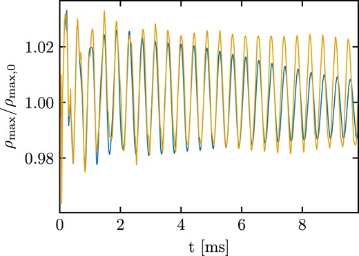
Fig.1 shows the evolution of the maximum density normalized to its initial value. The blue line refers to a moving-mesh simulation, while the orange line to a static-mesh run where the mesh-generating points do not move. We note that both simulations preserve the initial TOV solution, i.e. the whole radial density profile, with only a minor density drift during the roughly 10 ms evolution. The moving-mesh simulation features a stronger damping of the excited oscillations and a somewhat more pronounced density drift in comparison to the static-mesh case. We extract the main radial pulsation frequency by a Fourier transform of the density oscillations. We obtain 2.672 kHz for the moving mesh and 2.682 kHz for the static mesh, which are both in excellent agreement with previous results (2.696 kHz in Font et al. 2002). In Fig. 2, we present the power spectrum of the normalized maximum density (see Fig. 1). We consider the whole signal and apply a Tukey window with a shape parameter of 0.1. In addition, we zero pad the signal, which effectively leads to smoother curves in the power spectrum. We note that a number of overtones are excited as well. In particular, in the moving-mesh simulation we identify 6 overtones, which all agree within less than 2 per cent with the values reported in Font et al. (2002). The presence of several overtones is in line with the observation of several box-shaped oscillation cycles in Fig. 1 as the Fourier transform of a pulse wave is given by a number of higher overtones with decaying magnitude. In the static mesh simulation higher overtones seem to be less excited (or stronger damped) and only the first two appear prominently. We also extract the FWHM of the first three peaks in Fig. 2 and find 129, 130, and 132 Hz (161, 212, and 321 Hz) for the static-mesh (moving-mesh) calculations.
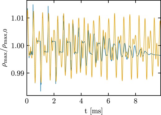
Evolution of the maximum rest-mass density normalized to its initial value for a 1.4 M⊙ TOV neutron star modelled as a polytrope with K = 100 and Γ = 2. The blue line refers to a moving-mesh set-up, while the orange line to a static-mesh set-up. Both simulations adopt the Cowling approximation. In both cases, a radial velocity perturbation with amplitude −0.005 was applied. See the main text for details regarding the mesh set-up.
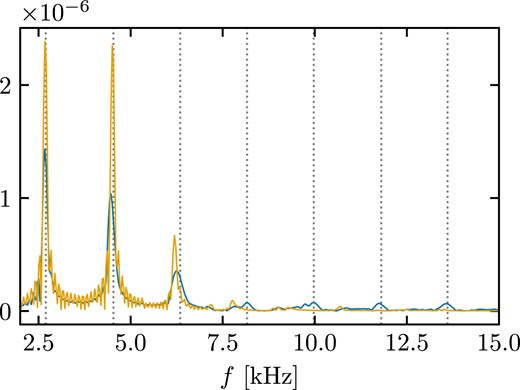
Frequency spectrum of the maximum rest-mass density evolution of a 1.4 M⊙ TOV neutron star described by a polytropic EOS with K = 100 and Γ = 2 employing the Cowling approximation (see Fig. 1). The blue line corresponds to a moving-mesh simulation, while the orange line refers to a static-mesh calculation. The vertical dashed lines correspond to the frequencies computed in Font et al. (2002). The units of the vertical axis are arbitrary.
The moving-mesh and static-mesh evolutions are rather similar for the first few milliseconds. However, at later times the moving-mesh set-up exhibits some damping in contrast to the static-mesh. This possibly originates to some extend from the surface layers. Initially, the star contracts while atmosphere cells do not move. This results in a small gap between mesh-generating points that correspond to stellar material and thus closely follow the fluid motion, and points belonging to the atmosphere. This leads to larger cells close to the surface and thus the resolution at the stellar surface effectively drops. When the star expands, the stellar surface moves into the atmosphere. During expansion and contraction phases of the star, cells can cross the atmosphere threshold. Cells belonging to the star can become atmosphere, and atmosphere cells can accumulate material to become ‘active’ stellar cells. Overall, this leads to a decrease in the resolution close to the surface already after the first few ms. This behaviour is shown in Fig. 3, which displays the rest-mass density in the z = 0 plane after evolving the system for roughly 2 ms. The left panel refers to the moving-mesh simulation, while the right panel corresponds to the static-mesh simulation. In both panels, we employ white lines to display cell boundaries, which reveals the mesh geometry. Fig. 3 captures how the moving mesh evolves compared to the static-mesh simulation (i.e. also how the moving mesh evolves compared to the initial mesh geometry). In particular, the static-mesh and moving-mesh simulations have similar resolutions in the interior of the neutron star up to a few hundreds of meters beneath the surface. In the outer meters of the crust, the moving-mesh simulation has a lower resolution, which is one of the reasons for the higher damping. Finally, in the moving-mesh simulation a thin high-resolution shell forms right at the surface because of cells which originally belonged to either the star or the atmosphere.
![Rest-mass density at the z = 0 plane for the moving-mesh (left panel) and static-mesh (right-panel) simulations on a fixed space–time. The thin white lines represent the cell boundaries and thus display the mesh geometry. The subpanels at the top right corner of each panel depict a zoomed-in version of the region [11, 13] × [0, 2] in the respective plot. Both snapshots are taken at a time t = 1.97 ms.](https://oup.silverchair-cdn.com/oup/backfile/Content_public/Journal/mnras/528/2/10.1093_mnras_stae057/1/m_stae057fig3.jpeg?Expires=1749216160&Signature=tsDxPzFD0puTUMtJBN0Avs0HTa2c19utnsKru3SkWXvlFh6I0s8Xo0ilXrgg--nanRq9v1JRCkZZOmgU5EeI0lA8rDYsaHz7ENofNOhjWmVsWfacx8HZOIGqBxGG3LlZ8CPCaZ-Q2~amh4wzt2LdNz2OyCExbg-4u6EEBgOQW8oX8qUpN~U-GdVLEYMpOnPTV-MSrl3FHyXMXuDFMogrOFq-lYVpYdbP9pdAXKOb2AILgZGXsGrbospv1AQRxG9YfgAqB8WtwO-sGLTfHqRNN~VKsOI8zf8DVDsA-RvPfRBbRIEvg8BRsxw5I206CnA88rxeneyZTg0E-xKOJbb0RQ__&Key-Pair-Id=APKAIE5G5CRDK6RD3PGA)
Rest-mass density at the z = 0 plane for the moving-mesh (left panel) and static-mesh (right-panel) simulations on a fixed space–time. The thin white lines represent the cell boundaries and thus display the mesh geometry. The subpanels at the top right corner of each panel depict a zoomed-in version of the region [11, 13] × [0, 2] in the respective plot. Both snapshots are taken at a time t = 1.97 ms.
To evaluate the effect that a lower resolution close to the surface has on the evolution, we perform an additional static-mesh simulation. We construct a mesh where we distribute the mesh-generating points to obtain a uniform Cartesian grid with a cell size of 0.1 M⊙ within a radius of 7.8 M⊙ ≈ 11.51 km (i.e. 96 per cent of the stellar radius) surrounded by a uniform Cartesian grid with a cell size of 0.2 M⊙ outside the radius of 7.8 M⊙. We present the evolution of the rest-mass density in Fig. 4(a). We find that the evolution of the maximum density features some damping in this new static-mesh simulation and the amplitude of the oscillation has decreased by a factor of roughly 2 after ≈10 ms of evolution. In addition, we extract a frequency of 2.674 kHz for the main radial pulsation, i.e. rather similar to the moving-mesh simulation. This observation supports that a lower resolution close to the surface can partially explain the damping in the maximum rest-mass density oscillation in the moving-mesh simulation.
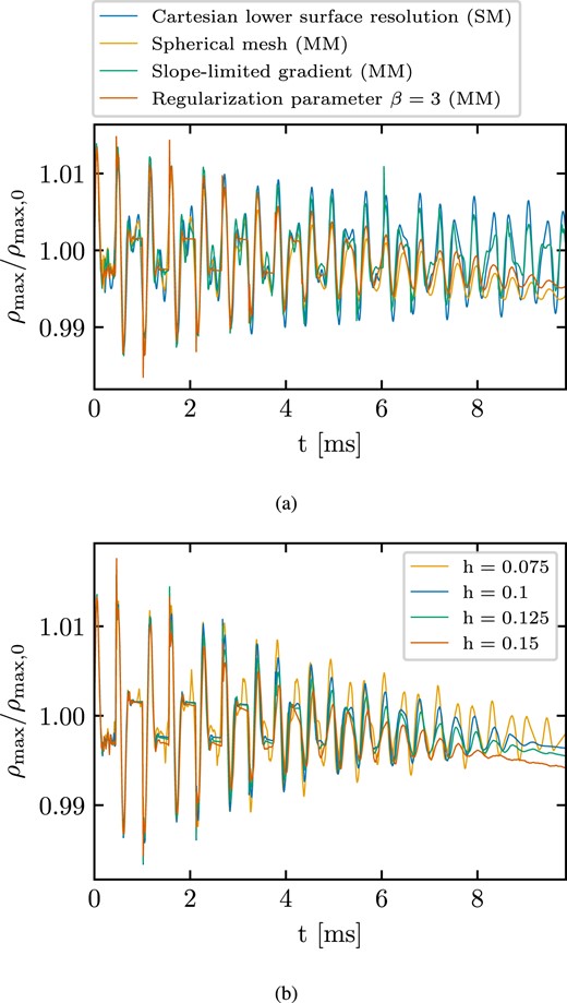
Rest-mass density evolution of a 1.4 M⊙ TOV neutron star modelled as a polytrope with K = 100 and Γ = 2 within the Cowling approximation for different simulation setups. Panel (a): Effect of different numerical choices (see legend and main text in Section 4.1.2). In the legend, we denote moving- and static-mesh simulations as MM or SM, respectively. Panel (b): Impact of resolution on the moving-mesh calculations starting from a Cartesian initial mesh geometry. The default set-up (h = 0.1) matches the blue line in Fig. 1.
Furthermore, we perform a set of additional simulations to investigate the oscillation behaviour in Fig. 1 and we already refer to Section 4.2 showing that the use of the Cowling approximation is a major reason for damping in moving-mesh calculations. We investigate a number of aspects of the numerical description and their effects on the overall evolution:
Effect of resolution: We perform three moving-mesh simulations, where the initial mesh-generating point distribution is similar to the one described in Section 4.1.1, but we vary the cell size of the central, high-resolution mesh to be h = 0.075, 0.125, and 0.15, respectively (i.e. one higher-resolution and two lower-resolution simulations compared to the default set-up). Fig. 4(b) shows the evolution of the maximum rest-mass density for the different resolutions. Increasing the resolution leads to less damping of the oscillation and reduces the minor density drift. The damping is not fully removed for the resolutions considered here. However, below we show that the set-up for this resolution study (e.g. the initially Cartesian mesh) is not ideal and other aspects of the numerical treatment strongly improve the evolution. The extracted frequency of the main radial oscillation is 2.664, 2.668, and 2.674 kHz for h = 0.15, 0.125, and 0.075, respectively, i.e. there is a very minor increase of the frequency with increasing resolution.
Mesh geometry: We consider a moving-mesh simulation with an initial set-up of mesh-generating points which leads to a spherical distribution of cells. The initial mesh is identical to the standard resolution set-up described in detail in Section 4.2.1, where more details can be found. We emphasize that the equidistant radial separation between consecutive shells is ≈191 m, i.e. the resolution in this simulation is more comparable to the run with h = 0.125 from point (i) above. We compare the number of cells within the star at the beginning of each simulation. The cells within the star in the simulation on the spherical mesh are |$\approx 92~{{\ \rm per\ cent}}$| of the cells covering the star in the simulation on the (initially) Cartesian mesh with h = 0.125. The differences in the number of cells covering the star between the spherical mesh simulation and the h = 0.075, 0.1, and 0.15 simulations are larger. Hence, the spherical mesh simulation should be compared with the h = 0.125 run in Fig. 4(b), while the first features a somewhat lower resolution. Evidently, the evolution of the rest-mass density on the spherical mesh features less damping compared to the (initially) Cartesian h = 0.125 mesh [compare orange line in Fig. 4(a) and green line in Fig. 4(b), respectively]. Using a spherical mesh does not completely remove the damping, but the comparison shows that a mesh which better captures the symmetries of the physical system is a more appropriate starting point for a moving-mesh simulation.
Gradient slope limiter: We set up a moving-mesh simulation with an identical set-up as the original one (i.e. Cartesian initial mesh with h = 0.1), but we employ the standard slope-limited gradient in Arepo (equation (30)) instead of the MC slope limiter (see Section 3.2). We find that the maximum density in this new simulation evolves in a rather similar manner to the original moving-mesh simulation with the MC slope limiter in the first few ms. However, at later times the maximum rest-mass density oscillation exhibits noticeably less damping in the new simulation and can still be clearly identified after roughly 10 ms [see green line in Fig. 4(a), see also the discussion on slope limiters in Font et al. (2002)]. Employing the original slope-limiting procedure of arepo may benefit from the fact that information about all the neighbouring cells enters the definition of ψij (see equation 30) and not just the gradient estimate. Thus, it might be a more appropriate choice for moving-mesh simulations compared to the MC slope limiter.
Regularization scheme: We consider the impact of the parameters β and fshaping, which enter the regularization scheme1 (see equation 36 and Section 3.5). We run a total of four additional moving-mesh simulations with an identical initial mesh as in the original run, where we systematically vary the values of the two parameters (β, fshaping) to be (1.5, 0.5), (3, 0.5), (2.25, 0.3), and (2.25, 0.7). Fig. 4(a) shows the impact of increasing β, i.e. applying less regularization as compared to the original simulation. The evolution features less damping than in the original set-up and the oscillation can still be identified at the end of the simulation. We note that decreasing β has the opposite effect, while changing the value of fshaping has no noticeable effect (not shown). These results align with point (ii), namely that the moving-mesh approach performs better if less regularization of the mesh is required and thus the cell motion more closely follows the local fluid motion.
To quantify the impact of the regularization, we compute the fraction of cell motion stemming from the mesh regularization compared to the fluid velocity. Fig. 5 shows this fraction as a function of the density. We compute the fraction as an average over the density (by defining density intervals [10N, 10N + 1] g cm−3 with N being an integer in [7,14]) and over time by considering several snapshots (produced every 100 code units, i.e. ≈0.49 ms). We report the different numerical set-ups in panel 5(a) and the results for different resolutions in panel 5(b). We observe two general trends. First, the motion due to the mesh regularization is generally sizable (at all densities) and more pronounced in the outer layers, in line with the discussion above and Fig. 3. Secondly, Figs 4 and 5 clearly show that the magnitude of damping in moving-mesh simulations is related to the relative strength of mesh regularization. Numerical setups that require less regularization feature less numerical damping.2 The effects discussed under points (i) to (iii) can thus be traced back to their impact on the mesh regularization. A more significant contribution from the mesh regularization to the cell motion arguably leads to more damping, as mesh regularization precisely means to introduce cell motion which does not follow the fluid motion and thus spoils the specific advantage of a moving mesh. For comparison, we also provide the relative fraction of the corrective cell velocity from regularization for the BNS merger simulation discussed in Section 5, which shows a much smaller relative impact of the mesh regularization.
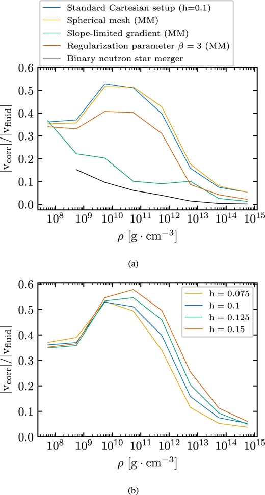
Fraction of the corrective velocity due to regularization over the fluid velocity for the Cowling simulations of the TOV polytropic neutron star. The ratio is averaged over the density and over time (see the main text). Panel (a): Includes all the moving-mesh setups from Fig. 4(a). The blue line refers to the standard (initially) Cartesian moving-mesh set-up with h = 0.1 (note that the blue line in Fig. 4(a) is a static-mesh run). The black line refers to the BNS merger simulation discussed in Section 5. Panel (b): Impact of resolution for all the (initially) Cartesian set-ups shown in Fig. 4(b). The blue line is the same as in panel (a).
Overall, we emphasize that the tests in this section demonstrate that further effort is required to identify set-ups that lead to better moving-mesh evolutions of TOV stars in the Cowling approximation. Based on our investigation, certain aspects of the numerical modelling (e.g. initial mesh geometry, slope limiter, regularization scheme parametrization) positively influence the moving-mesh evolution. We have chosen our default settings to be as close as possible to the set-up in Font et al. (2002) for a better comparison, but obviously other choices seem more appropriate for TOV systems. As apparent in Fig. 5, TOV stars may not be an easy target for moving-mesh simulations because of their quasi-stationary nature where, in contrast to dynamical systems like BNS mergers, the motion of the mesh is strongly determined by regularization.
We note that the cell rearrangement in the moving-mesh evolution highlights that a direct comparison between a static-mesh and a moving-mesh simulation is not necessarily straightforward. Even if the initial mesh geometries match, the moving mesh quickly rearranges and does not have a single resolution that one can compare to the fixed mesh. In addition, allowing the cells to move without taking the mass distribution of the system into account can lead to issues close to the surface as reported. The rearrangement of cells close to the surface can create small cells. If these cells are not derefined, which we do not do in our TOV simulations, they can in principle reduce the (global) time-step, hence increasing the required computational effort. We note that the mesh-generation algorithm typically requires more time to construct a Cartesian grid compared to other distributions with the same number of mesh-generating points due to the extra cost required to resolve geometric degeneracies during mesh construction.
4.2 Dynamical space–time
4.2.1 Initial data
We construct TOV data for a 1.41 M⊙ neutron star configuration (central density ρc = 9.545 × 10⁻⁴) described by the H4 EOS (Lackey, Nayyar & Owen 2006) modelled as a piecewise polytrope (Read et al. 2009). We complement H4 with a Γth = 1.75 thermal ideal-gas component.
The initial mesh-generating point distribution and subsequently the mesh geometry is different from our Cowling tests. We map the 1D TOV data to a spherical distribution of cells located at the centre of the simulation domain. We use a total of 85 shells extending up to a distance of 11 M⊙ ≈ 16.2 km, with an equidistant radial separation ≈191 m between consecutive shells. In each shell, we distribute |$12N_\mathrm{side}^2$| cells based on the HEALPix tessellation by Górski et al. (2005), where for a shell with inner radius rlower and outer radius rupper we set |$N_\mathrm{side}=\sqrt{\pi /12} \times (r_\mathrm{lower}+r_\mathrm{upper})/(r_\mathrm{upper}-r_\mathrm{lower})$| (see also Pakmor et al. 2012). In addition to these shells, we place a coarse Cartesian grid to fill the rest of the computational domain. This set-up is our standard resolution run. In addition, we construct two similar set-ups with 100 shells (i.e. a resolution of ≈162.4 m) and 64 shells (namely a resolution of ≈253.7 m), which we employ for higher and lower resolution (moving-mesh) simulations, respectively. Finally, we also test a mesh which is similar to our standard resolution, but we randomly place the mesh-generating points on each shell to eliminate possible grid orientation effects.
In this section, we compare the radial mode frequency from our simulations to a calculation with an independent linear perturbation code, which we developed following the approach outlined in Gondek, Haensel & Zdunik (1997). Unlike Section 4.1, we do not compare to results from an independent Cartesian hydrodynamics code.3 Since the perturbative result is practically exact and the comparison does not rely on choosing the same grid set-up, we employ a grid that captures well the geometry of the physical system.
In contrast to the previous test, the space–time evolves dynamically. We solve the metric field equations on a uniform Cartesian grid with 1293 points with a resolution hM = 0.3 M⊙. Similar to the Cowling tests, we excite the radial oscillation with a perturbation of the form (40) with A = −0.001 and we set ρatm = 10−8 × ρmax and ρthr = 10 × ρatm.
4.2.2 Simulations
In Fig. 6, we present the time evolution of the normalized maximum density of the 1.41 M⊙ H4 stellar model with a moving mesh (blue) and a static mesh (orange) with our standard resolution set-up. Again, we compute the fundamental radial pulsation frequency. Using a Fourier transform of the density oscillations, we obtain 2.343 kHz for the moving mesh and 2.358 kHz for the static mesh. For comparison, the perturbative calculation gives 2.385 kHz. Deviations of the order of 1 per cent are comparable to what is found by other codes, e.g. Font et al. (2002).
Normalized maximum rest-mass density from a moving-mesh (blue line) and a static-mesh (orange line) evolution of a 1.41 M⊙ star described by the H4 EOS. The space–time is evolved dynamically and the metric field equations are solved on a grid with 1293 points and resolution 0.3 M⊙. The pulsation is excited with a radial velocity perturbation with amplitude −0.001. See the main text for a description of the initial mesh geometry.
Moving-mesh runs with the higher and lower resolution (see Fig. 7) result in frequencies of 2.352 and 2.318 kHz, respectively, i.e. increasing the resolution leads to frequencies which lie closer to the perturbative result. In addition, we perform a moving-mesh simulation with an initial mesh set-up with standard resolution (≈191 m) including a random component to slightly offset the mesh-generating points. We obtain 2.349 kHz, which is slightly higher than the result from the same resolution set-up without the random component. We note that including the random component in the mesh set-up reduces grid effects, while it only slightly increases the damping in the maximum density oscillation. The overall agreement in the frequencies validates our implementation of GRHD and the metric solver, as well as their coupling in a realistic set-up that employs a microphysical EOS.
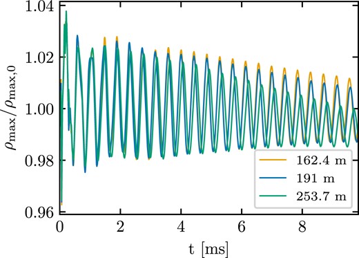
Evolution of the normalized maximum rest-mass density in moving-mesh simulations with different resolutions. The legend provides the radial separation between consecutive shells in the initial (spherical) mesh. The space–time is dynamically evolved. Note that the standard resolution set-up (blue line) matches the blue line in Fig. 6.
The moving-mesh and static-mesh standard resolution simulations of the star preserve the initial TOV solution during the whole simulation time with only a very mild drift in the central density, which is also seen in other simulations (e.g. Font et al. 2002). The drift diminishes with higher resolution, see Fig. 7. Increasing the resolution also yields less damping in the rest-mass density oscillation.
The oscillations in the moving-mesh simulations show some damping over time, but the amplitude is still sizable at the end of the calculations. In comparison to the Cowling runs, the damping is less pronounced, and the evolution of ρmax generally does not deviate as much from the respective static-mesh runs. In Section 4.1.2, we found that a combination of effects enhances damping in moving-mesh simulations compared to static-mesh runs in the Cowling approximation (e.g. mesh geometry, slope limiter, and regularization). The damping of the moving-mesh simulation in Fig. 6 (dynamical space time) in comparison to the different moving-mesh runs in Section 4.1.2 (Cowling) is relatively moderate. This suggests that the Cowling approximation (versus a dynamical evolution of the space time) is another major reason for the damping observed in moving-mesh simulations in Section 4.1.2. Although we compare simulations with different set-ups (EOS, initial excitation, mesh geometry), this is in line with the observation that the response to perturbations is different in Cowling and dynamical space time simulations (see e.g. Dimmelmeier, Stergioulas & Font 2006). Apart from the aspects discussed in Section 4.1.2, specific implementations such as modifying the cell motion close to the surface and suppressing small secular drifts of cells are likely to improve the behaviour in quasi-stationary situations. Since our work is targeted to highly dynamical problems, where we do not face the same issues, we do not follow up on these points here.
5 BNS MERGERS
In this section, we discuss a BNS merger simulation. This is the first simulation of a neutron star merger using a moving mesh, and we show that this approach can be successfully used to simulate such systems.
5.1 Initial data and setup
We employ the DD2 EOS (Hempel & Schaffner-Bielich 2010; Typel et al. 2010) as a zero-temperature β-equilibrium tabulated microphysical EOS. We remark that the DD2 model provides the full temperature and composition dependence of the EOS. In this work however, for convenience, we only use a slice at T = 0.1 MeV as the lowest temperature provided by the EOS table. We supplement the barotropic EOS with a thermal ideal-gas component with Γth = 1.75, as described in Section 2.3 (see Bauswein, Janka & Oechslin 2010, for more details). DD2 is marginally compatible with current observational constraints on the tidal deformability from GW170817 (Abbott et al. 2017a, 2019) and fully consistent with mass measurements of various binary systems (Demorest et al. 2010; Antoniadis et al. 2013; Arzoumanian et al. 2018; Linares, Shahbaz & Casares 2018; Cromartie et al. 2020).
We construct initial data for an equal-mass BNS system in a quasi-circular quasi-equilibrium orbit using LORENE4 (Gourgoulhon et al. 2001). The two companion neutron stars have a gravitational mass of M = 1.35 M⊙ (at infinite binary separation) and are irrotational. The initial separation is 26 M⊙ ≈ 38.4 km. LORENE solves the metric field equations using the conformal flatness approximation like our code. As a result, we do not observe an unphysical transient at the beginning of our simulation as compared to fully relativistic simulations, which react to the missing GW content of the initial data. Hence, we can start our simulation from a relatively small initial separation of the two companion stars.
We map the initial data from LORENE to a distribution of mesh-generating points which follows approximately the mass distribution. In particular, around the centres of each star, we construct spherical shells and then distribute cells on each shell based on the HEALPix algorithm by Górski et al. (2005) to obtain a distribution of mesh generating points that have roughly the same distance within the shell. We impose that the distance between points within the shell equals the thickness of the shell. The grid set-up is described in detail in Ohlmann et al. (2017). The original method described in Ohlmann et al. (2017) determines the radial positions of the shells such that each cell has roughly a mass mcell,0 following the density profile of the initial data. Here, mcell,0 is a free parameter, which directly relates to the resolution. The procedure described in Ohlmann et al. (2017) assumes that the density profile of each star is spherically symmetric. Hence, in our case, we employ a TOV solution with M = 1.35 M⊙ modelled by DD2. We emphasize that the TOV solution is only relevant for the purpose of distributing the mesh-generating points in a way that closely follows the mass distribution within the binary (around each companion star). The actual initial data, e.g. the three-dimensional density profile, originate from LORENE.
In the case of neutron stars, this procedure would lead to large cells close to the stellar surface, where the density drops steeply. Therefore, we modify the employed TOV density profile in the outer regions of the star. Between the distances rin = r(ρc/2) and rout = 1.1 × R, we keep |$\rho \sqrt{\gamma }=\rho \psi ^6$| fixed to the value at rin. Here, ρc is the central density and R the radius of the TOV star. We determine the position of the radial shells based on this modified density profile, which enhances the resolution in the outer layers of the star compared to the original procedure. As stressed, we finally assign the values from the LORENE solution to the cells which we obtain through this procedure.
This grid extends beyond the stellar radius. This particular set-up guarantees that the resolution does not drop abruptly close to the surface because of the steep density gradient. Moreover, we resolve the regions around R, which is important because the stars in the binary are not perfect spheres, but deformed. In the current simulation, we set mcell, 0 = 1.68 × 10⁻⁶ M⊙. In principle, this construction leads to a mesh with no grid orientation effects (see Ohlmann et al. 2017 for more details). We cover (vacuum) regions outside the spheres with radius rout around each star with a coarse uniform Cartesian mesh with resolution 10.1 M⊙. The atmosphere density is set to ρatm = 10−7 × ρmax and ρthr = 10 × ρatm. We do not impose any symmetries during the simulation. The metric field equations are solved on a uniform Cartesian grid with 1293 points and resolution 0.8 M⊙.
During the simulation we allow for cell refinement and derefinement. We set a cell target mass mcell,0 = 1.68 × 10⁻⁶ M⊙, which is the same that we used to find the radial positions of cells in the mesh-constructing algorithm (see Ohlmann et al. 2017, for more details). We refine cells with mass mcell > 2 × mcell,0 and derefine cells with mass mcell < mcell,0/2. Furthermore, for each cell we check the volume of every neighbouring cell. We ensure that a cell is not derefined if |$V\gt 1.5\times V_\mathrm{ngb}^\mathrm{min}$|, where V the cell volume and |$V_\mathrm{ngb}^\mathrm{min}$| the volume of the smallest neighbouring cell. We refine any cell for which |$V\gt 5\times V_\mathrm{ngb}^\mathrm{min}$| holds. To avoid creating an irregular mesh through the refinement process, in all cases we do not refine highly distorted cells i.e. cells with αmax ≥ 3.375 (see Vogelsberger et al. 2012, for more details). Cell refinement takes place if any of the refinement criteria is satisfied, while to derefine a cell we require that all derefinement criteria allow derefinement at the same time. This combination of criteria guarantees that we have a mesh where many cells have comparable mass content, while we also resolve the surface with a decent resolution (i.e. during the first milliseconds cells in the crust have an average size of ≈0.3 M⊙, which is larger than typical cell sizes in current static-mesh calculation; in the neutron star cores cells have typical dimensions of about 0.1 M⊙ which is comparable with typical cell sizes in static-mesh simulations). Roughly, 1.7 × 10⁶ cells with ρ > ρthr resolve physically interesting regions. Notably, shortly after the beginning of the simulation, we find only a small number of cells outside the two stars due to cell derefinement. Hence, in our approach the hydrodynamical domain can be arbitrarily large with practically no effect on the computational time.
We compare the maximum density (see Fig. 8) and lapse function evolution during the first few milliseconds of our binary system evolution to an independent simulation of a single 1.35 M⊙ TOV star described by DD2. The mesh-generating point set-up in the isolated star simulation is identical to the one which we employ for each individual star in the binary, while we keep the same metric resolution, atmosphere parameters and refinement/derefinement criteria. Discretization errors by the finite resolution excite oscillations in the maximum density and the minimum lapse function. Comparing the calculations of the isolated star and the binary, the frequencies are similar, while the amplitudes are slightly higher in the case of the isolated neutron star. Hence, we conclude that the set-up of our binary initial data works robustly and that the procedure does not introduce additional errors apart from those which are expected, i.e. truncation errors.
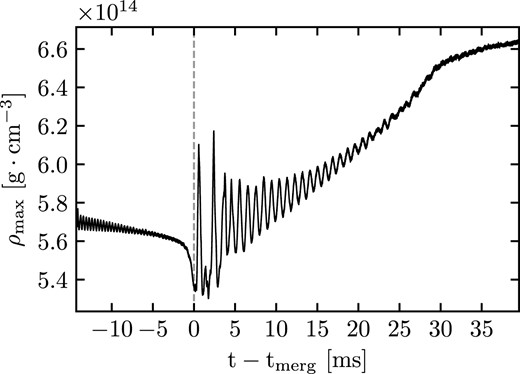
Maximum rest-mass density as a function of time for a BNS system with two 1.35 M⊙ neutron stars modelled with the DD2 EOS. The vertical dashed line indicates the time of merging.
We also perform additional simulations where we vary certain aspects of the numerical treatment (e.g. the hydro and metric resolutions) to evaluate their impact on the results. The additional simulations are discussed in Appendices D1 and D2.
5.2 Simulations
5.2.1 General dynamics
Fig.8 shows the evolution of the maximum rest-mass density ρmax during the simulation. The vertical dashed line indicates the time when the two neutron stars merge tmerg5 and separates the inspiral and the post-merger phase. The main stages of the binary evolution are shown in Fig. 9, where we present the rest-mass density in the orbital plane of the binary at four different times. The top left and top right panels correspond to snapshots taken during the late inspiral6 and right after merging, respectively. Middle and bottom row panels present two times at the late stages of the post-merger evolution on a logarithmic and on a linear scale. We evolve the binary for ≈39.5 ms after the stars merge.
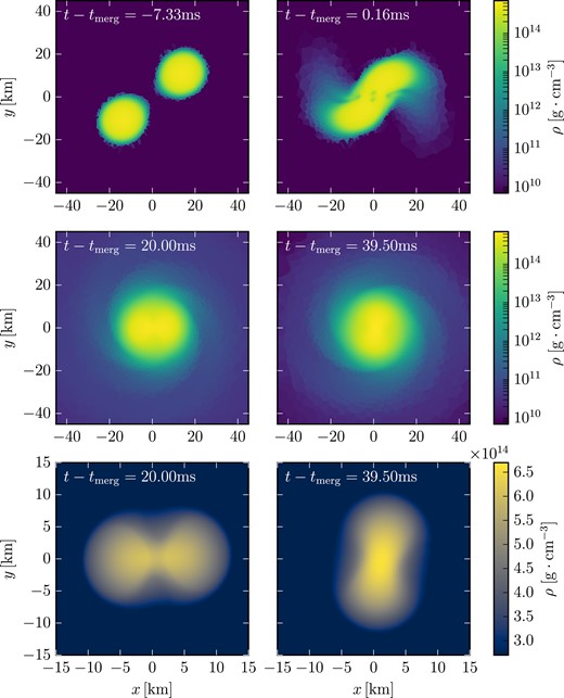
Evolution of the rest-mass density for the BNS merger simulation. Each panel shows a slice through the orbital plane of the binary. The densities in the upper and middle rows are displayed on a logarithmic scale, while the bottom row focuses on the high-density material of the remnant employing a linear density scale. The times are chosen such that the top row panels show snapshots from the late inspiral stage and the moment of merging, while the middle row panels display very late stages of the post-merger evolution. The times in the bottom row panels match those in the middle row.
Throughout the inspiral the two neutron stars revolve around each other, while the orbital separation decreases due to energy and angular momentum losses by GWs. As mentioned, during the inspiral the maximum density features small oscillations (Fig. 8) because discretization errors excite dominantly the radial mode. As the binary components approach each other, tidal effects become more pronounced (an incomplete list of early hydrodynamical studies of the merger include e.g. Rasio & Shapiro 1994; Zhuge, Centrella & McMillan 1994; Wilson, Mathews & Marronetti 1996; Ruffert, Rampp & Janka 1997; Rosswog et al. 1999; Oechslin, Rosswog & Thielemann 2002; Shibata, Taniguchi & Uryū 2005; Baiotti, Giacomazzo & Rezzolla 2008). The tidal deformations are visible in the top left panel of Fig. 9, which corresponds to the last few revolutions before the stars merge.
The stars collide with a relatively large impact parameter. The collision results in the sudden increase of the maximum density immediately after tmerg in Fig. 8 and shock-heating of material at the collision interface (e.g. Ruffert, Janka & Schaefer 1996; Rosswog et al. 1999; Shibata, Taniguchi & Uryū 2005; Oechslin, Janka & Marek 2007). Fig. 10 shows snapshots of the temperature Tth in the orbital plane right after merging (top row), when the system reaches the highest temperatures, as well as two snapshots in the post-merger phase (bottom row). As shown in the upper panels of Fig. 10, matter at the collision interface of the two neutrons stars reaches temperatures of almost 90 MeV. In Fig. 10 we also overplot contour lines corresponding to two different densities. The white dashed line indicates where the density equals 1013 g cm−3 to highlight the region containing the bulk of matter at the times shown in the plots. The solid white line corresponds to a density of 2.7 × 10¹⁴ g cm−3 (nuclear saturation density). Most of the high-density parts of the stars, except for matter at the collision interface, remain cold even during the merger phase (see e.g. Shibata, Taniguchi & Uryū 2005; Oechslin, Janka & Marek 2007; Kastaun, Ciolfi & Giacomazzo 2016; Hanauske et al. 2017). The highest temperatures are reached in hotspots with densities slightly below 2.7 × 10¹⁴ g cm−3. The densities are lower in these blobs because of the significant thermal pressure at these temperatures. These regions are also visible in the top right panel of Fig. 9 and form due to the mixing of material from the two stars (see e.g. Kastaun, Ciolfi & Giacomazzo 2016). The contact interface between the two stars is subject to the Kelvin–Helmholtz instability. The distribution and evolution of the temperature in the upper row of Fig. 10 is indicative of the local vorticity (see e.g. Kiuchi et al. 2015).
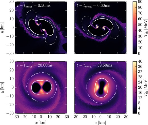
Temperature in the orbital plane for the BNS merger simulation. The top row shows snapshots right after the neutron stars merge, when the temperature reaches the highest value of Tth ≈ 90 MeV. The bottom row presents snapshots taken at 20 and 39.5 ms after merging. White dotted and solid contours indicate densities of 1013 and 2.7 × 10¹⁴ g cm−3, respectively. The two cold, high-density cores are clearly visible at late stages of the evolution (bottom panels).
In the post-merger phase, a double-core structure forms. We observe that our simulation preserves the double-core structure for more than 20 ms after tmerg. This is clearly shown in the middle and bottom rows of Fig. 9, as well as the bottom row of Fig. 10. The two cores (enclosed in the white solid contour line in the bottom left panel of Fig. 10) can be clearly identified 20 ms after merging. The centres of the cores merge at t−tmerg ≈ 28 ms. Even at the very late stages of the evolution, i.e. at t − tmerg = 39.5 ms, the high-density material has not yet settled to a single spherically shaped core, but exhibits a bar-shaped structure. The double-core phase in our simulation lasts significantly longer compared to other simulations with fixed-grid finite-volume approaches (see e.g. Kastaun, Ciolfi & Giacomazzo 2016; Hanauske et al. 2017). Similarly, the quasi-radial mode survives for a long time after merging as shown in Fig. 8.
The cores remain cold during the whole post-merger evolution. The remnant still exhibits high temperatures, up to ≈40 MeV. These highest temperatures at late times occur at the outer edges of the shearing interface between the two cold cores. The system exhibits density spiral arms starting at the central object during the whole post-merger phase that we simulate, as can be seen in both middle row panels of Fig. 9 and in the bottom row panels of Fig. 10.
We cannot identify the development of a pronounced m = 1 instability in the evolution of the rest-mass density in the orbital plane until the end of the simulation (Paschalidis et al. 2015; East et al. 2016; Lehner et al. 2016; Radice, Bernuzzi & Ott 2016a). Based on a modal decomposition of the density (see e.g. Radice, Bernuzzi & Ott 2016a), the m = 2 mode features only extremely minor damping and remains dominant compared to the m = 1 mode throughout the whole simulated post-merger phase. For comparison, we simulate the binary system with an SPH code, which also adopts the conformal flatness approximation (Oechslin, Rosswog & Thielemann 2002; Oechslin, Janka & Marek 2007). We employ the same EOS treatment and choose a resolution of roughly 3 × 10⁵ SPH particles in total.7 In the SPH simulation, the m = 1 instability does clearly occur for the same binary system. A modal decomposition of the SPH simulation reveals that the m = 2 mode is damped over time and at t − tmerg ≈ 15 ms its amplitude decays below that of the m = 1 mode. Considering that the two codes employ very similar metric modules, these results support that the development of the one-arm instability depends on the employed hydrodynamics schemes and the resolution.
We briefly examine the angular velocity profile8 in the equatorial plane at different stages of the post-merger evolution in Fig. 11. The rotation profile initially exhibits a maximum at the centre of the remnant. The value of the time- and azimuthally averaged angular velocity Ω at the centre decreases over time and at later times an off-centre peak forms. The off-centre maximum first appears at t − tmerg ≈ 28 ms at a radial distance of ≈4 km. Over time the position of the peak moves outwards from the centre to about ≈7 km at the end of the simulation. The qualitative characteristics of the angular velocity profile agree with what is reported in other simulations (see e.g. Shibata, Taniguchi & Uryū 2005; Kastaun, Ciolfi & Giacomazzo 2016; Guilet et al. 2017; Hanauske et al. 2017), but the evolution of the profile and the overall angular momentum redistribution happens over longer time-scales. A similar delay in the evolution of the Ω profile has been reported in Kiuchi et al. (2018) for simulations with very high resolution. The latter calculations, however, employ a different EOS and include magnetic fields, which is why a direct comparison is difficult.
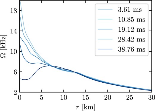
Rotation profile of the remnant at different times after merging. The angular velocity Ω is averaged along the azimuthial direction and over a time interval of 1 ms. The legend indicates t − tmerg for each line, where t refers to the midpoint of the respective 1 ms time interval.
Overall, the general dynamics and the qualitative features of our simulation are consistent with what is found in other simulations. A notable difference is that the double-core structure and the quasi-radial oscillations persist for a longer time. Similarly, an off-centre peak of the angular velocity profile emerges only at relatively late times. These points hint that the evolution with the moving-mesh set-up might have low numerical viscosity (see also the discussion on the damping of the GW signal in Section 5.2.2).
Finally, we comment on the resolution of our simulation. In principle, we cannot define a single resolution in moving-mesh simulations, because cells do not have a fixed shape and volume. This is clearly visible in both Figs 9 and 10, where in lower density regions the cell shapes are visible. We can however estimate the resolution under some assumption for the cell geometry. Here, we assume that cells are spheres and focus on the high-density regions. For material with ρ > 0.5 × ρmax at a given time we compute the average cell volume and in turn the cell radius. We then estimate the mean distance between cell centres in these regions as twice the computed radius. Throughout the post-merger phase, we obtain an average distance between cell centres of approximately 0.11 M⊙ ≈ 162 m in regions with rest-mass density above 50 per cent of ρmax. Naturally, some cells are smaller (or larger) than what this number indicates. This highlights the ability of our implementation to reach resolutions which are roughly comparable to what is currently used in merger simulations, although typically with high-order schemes. Our simulation required a few weeks of computing time running on 192 cores (see also Appendix D1). In the future, we plan to perform simulations with even higher resolution.
5.2.2 Gravitational wave signal
In Fig. 12, we show the plus polarization of the GW signal h+ (strain at a distance of 40 Mpc along the polar axis), multiplied by a factor of 1.4 (denoted as |$h_+^\mathrm{1.4}$|) to account for the underestimation of the amplitude by the quadrupole formula (see Shibata, Taniguchi & Uryū 2005, likely the factor is closer to 2 comparing recent simulations (Diener, Rosswog & Torsello 2022; Soultanis, Bauswein & Stergioulas 2022). The vertical dashed line in Fig. 12 indicates the merging time. Before tmerg the system emits GWs with a frequency twice as large as the orbital frequency. As the stars approach each other, the frequency, as well as the amplitude of the GW signal, increase. The coalescence of the stars excites a number of modes in the post-merger remnant, which shape the post-merger GW signal.
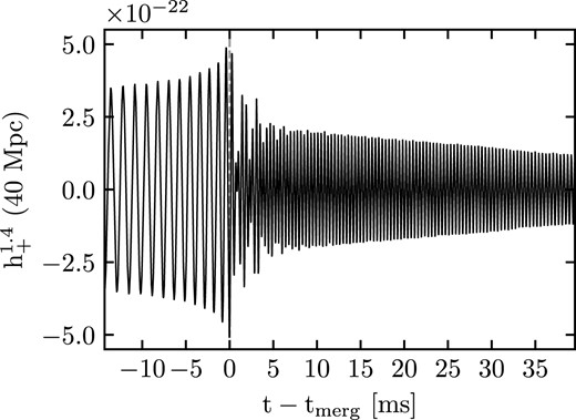
Gravitational wave amplitude |$h_+^\mathrm{1.4} = 1.4 \times h_+$|, where h+ is the strain of the plus polarization at a distance of 40 Mpc for the BNS simulation. The vertical dashed line shows the merging time.
Notably, the damping of the post-merger GW signal is very slow for the approximately 39.5 ms of post-merger evolution, which is in agreement with our observation in Section 5.2.1 that numerical viscosity may be relatively low in this simulation (see also Appendix D1). We determine the damping time to be τpeak ≈ 48 ms based on the analytic model presented by Soultanis, Bauswein & Stergioulas (2022). The SPH simulation with roughly 3 × 10⁵ SPH particles (see Section 5.2.1) yields τpeak ≈ 10.5 ms. Soultanis, Bauswein & Stergioulas (2022) perform fully general relativistic simulations with finest grid resolutions of 277 m and 185 m on a fixed grid and obtain τpeak < 11 ms for all their models and resolutions (τpeak ≈ 7 ms for the binary system with total gravitational mass of 2.7 M⊙), which is significantly below our current result. We do however note that Soultanis, Bauswein & Stergioulas (2022) employ a different EOS, which does not allow for a direct comparison with our simulation. We note that the GW back-reaction scheme somewhat underestimates the physical damping by GWs because of the underestimated amplitude. In Appendix D1 we clarify that accounting for this underestimation does somewhat reduce the damping time-scale, but we still find a slowly damped post-merger GW emission.
In Fig. 13, we present |$h_\mathrm{eff,+}(f)=f\cdot \tilde{h}_\mathrm{+}(f)$|, where |$\tilde{h}_\mathrm{+}(f)$| is the Fourier transform of the |$h_+^\mathrm{1.4}$| polarization, as measured at 40 Mpc. The solid line corresponds to the spectrum of the full GW signal from the whole evolution, while the dotted line is the Fourier transform of the signal from the post-merger phase alone. In addition, we show the design sensitivity of Advanced LIGO (LIGO Scientific Collaboration et al. 2015) and the Einstein Telescope (Punturo et al. 2010) with the upper and lower dash–dotted lines, respectively. We extract the main oscillation frequency in the spectrum (marked by a vertical dashed line) at fpeak = 2.56 kHz. For comparison, in our SPH simulation of the same binary system (see Section 5.2.1), we obtain fpeak = 2.62 kHz, which is in good agreement with our current result. In comparison to the SPH simulation, the features in the GW spectrum in Fig. 13 are more pronounced likely due to the low numerical damping of the signal. In addition, we compare to fully general relativistic simulations of the binary system from the CORE database9 (Dietrich et al. 2018). We extract fpeak = 2.57 kHz and fpeak = 2.65 kHz for the two available simulations with finest grid resolutions of 0.125 and 0.083 M⊙, respectively (see Radice et al. 2016b, 2017, for more details). Both frequencies agree rather well with our result noting that these static-mesh simulations employed the full temperature-dependent EOS table.
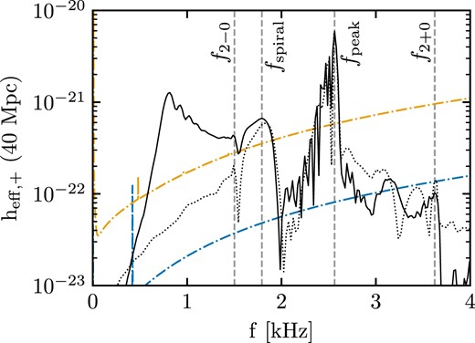
Gravitational wave spectrum of the plus polarization at a distance of 40 Mpc. The solid line refers to the whole simulation, while the dotted line displays the spectrum of only the post-merger phase. Both lines refer to |$h_+^\mathrm{1.4} = 1.4 \times h_+$|, as presented in Fig. 12. The vertical dashed lines indicate the frequency peaks fpeak, fspiral, f2-0, and f2 + 0. The upper (orange) and lower (blue) dash–dotted lines denote the design sensitivity of Advanced LIGO (LIGO Scientific Collaboration et al. 2015) and the Einstein Telescope (Punturo et al. 2010), respectively.
The spectrum in Fig. 13 contains several sub-dominant features, which are in principle observable. In particular, there is a pronounced broad peak at about 1.8 kHz. This peak emerges from the rotation of two antipodal tidal bulges, which form right after the merging. These tails rotate at a slower rate than the high-density parts and produce a peak at a frequency fspiral (Bauswein & Stergioulas 2015). In this particular simulation we obtain fspiral = 1.79 kHz, roughly 200 Hz lower than in the SPH simulation. The amplitude of the peak in the moving-mesh simulation is in comparison to the SPH calculation increased. Since the gravity solver is identical in both simulations, the different properties of this secondary peak hint to some sensitivity of this feature to the hydrodynamic scheme.
In Fig. 13, we also indicate the frequencies f2 ± 0 originating from the non-linear coupling between the dominant oscillation mode fpeak and the quasi-radial oscillation mode f0 (Stergioulas et al. 2011). To identify this feature, we estimate f0 from the evolution of the lapse function and tag the peaks that occur at ≈fpeak ± f0 in the GW spectrum.
6 SUMMARY
In this work, we extend the (originally Newtonian) moving-mesh arepo code to general relativistic hydrodynamics employing the flux-conservative Valencia formulation. We couple the implementation with a solver of the Einstein field equations imposing the conformal flatness approximation. This new tool can in principle be applied to a variety of astrophysical scenarios including those that require the dynamical evolution of the space–time. In this work, we focus on applications to neutron stars and neutron star mergers and supplement the code with a module to include a high-density EOS.
We validate the implementation by performing different test calculations, which can be compared to independent results. We simulate isolated, static neutron stars with a fixed space–time (Cowling approximation) and with a dynamical space–time (TOV tests). In both tests, the code preserves very well the density profile of the initial equilibrium model. The frequencies of radial oscillations, which are excited by truncation errors and an added perturbation, coincide very well with perturbative results and simulations from other codes, which verifies our implementation. We run simulations with moving meshes and static meshes which allow a more direct comparison to existing calculations. arepo offers the advantage that the initial grid configuration can be freely chosen and adapted to the specific problem to be simulated. We employ different choices including a Cartesian mesh and a spherical distribution of the mesh-generating points. The implementation presented here represents the first general relativistic moving-mesh code with a dynamical space–time evolution.
We present the first moving-mesh simulation of a neutron star merger including the late inspiral phase and the post-merger evolution, which we run until roughly 40 ms after merging. The initial mesh set-up approximately follows the mass distribution and geometry of the system. For the merger calculation we employ an additional feature of arepo, namely the adaptive refinement and derefinement of computational cells during the simulation. We find that in the high-density regime criteria to approximately achieve a target mass of the grid cells, which is comparable to the initial set-up, work well in merger simulations. Although one cannot define a unique resolution in moving-mesh simulations, the typical cell size in the high-density merger remnant is roughly 150 meters in our simulation. The computational costs for this setup are modest (a few weeks on about 200 cores) and thus even higher resolutions are well achievable. The choice of the initial mesh set-up and the refinement/derefinement criteria introduce a certain flexibility, which we will explore in future work with the prospect of further increasing the performance of the tool in merger simulations and possibly identifying choices well-adapted to specific problems or questions in this context.
We analyse the dynamics and the gravitational wave emission of the moving-mesh merger simulation. We find a general agreement with other simulations based on either SPH or static-mesh schemes. In comparison, our moving-mesh calculation seems to preserve the structure of the early post-merger remnant for a longer time. The initial double-core structure persists for more than 20 ms after merging. The quasi-radial oscillation of the remnant is only slowly damped and the profile of the angular velocity evolves on longer time-scales. This behaviour may prolongate the life time of the remnant although we do not run this specific simulation until the gravitational collapse takes place. Notably, the amplitude of the post-merger gravitational wave emission decreases only slowly and is still large even at the end of the simulation at roughly 40 ms after merging. These characteristics may point to a low numerical viscosity. The frequency of the dominant post-merger oscillation is in good agreement with results from simulations employing other hydrodynamic schemes. At any rate, these first results are very encouraging and show that the moving-mesh approach can be very beneficial for the simulation of BNS mergers.
The work presented in this paper will be the basis for more extensive studies and further developments with the new general relativistic moving-mesh code. The inclusion of fully temperature- and composition-dependent EOS tables and neutrino transport is in progress. Other more technical aspects to be addressed in the future concern the Riemann solver, choices for the grid set-up, cell merging and splitting, and the atmosphere treatment. The original arepo code already includes magnetic fields, which may be extended to the relativistic implementation. The currently employed conformal flatness approximation may be replaced by a full solver noting that the infrastructure for communication between the unstructured hydrodynamics grid and overlaid Cartesian grids is already available. The general flexibility and adaptivity of arepo suggest to employ the relativistic version for other relativistic astrophysical scenarios, e.g. black hole accretion discs and neutron star–black hole mergers.
ACKNOWLEDGEMENTS
We thank the anonymous referee for carefully reading the manuscript and their comments. We thank S. Blacker, E. Müller, S. Ohlmann, and N. Stergioulas for helpful discussions. GL and AB acknowledge support by the European Research Council (ERC) under the European Union’s Horizon 2020 research and innovation programme under grant agreement no. 759253. GL acknowledges support by the European Research Council (ERC) under the European Union’s Horizon 2020 research and innovation programme (ERC Advanced Grant KILONOVA no. 885281) and by the Deutsche Forschungsgemeinschaft (DFG; German Research Foundation) – MA 4248/3-1. GL, AB, and FKR acknowledge support by Deutsche Forschungsgemeinschaft (DFG; German Research Foundation) – Project-ID 138713538 – SFB 881 (‘The Milky Way System’, subproject A10). AB acknowledges support by DFG – Project-ID 279384907 – SFB 1245 and support by the European Research Council (ERC) under the European Union’s research and innovation program (ERC Synergy Grant HEAVYMETAL no. 101071865). AB and TS acknowledge support by the State of Hesse within the Cluster Project ELEMENTS. TS is Fellow of the International Max Planck Research School for Astronomy and Cosmic Physics at the University of Heidelberg (IMPRS-HD) and acknowledges financial support from IMPRS-HD. The work of TS and FKR is supported by the Klaus Tschira Foundation. The simulations of this paper were performed on the Virgo cluster at GSI Helmholtzzentrum für Schwerionenforschung, Darmstadt.
DATA AVAILABILITY
The data underlying this article will be shared on reasonable request to the corresponding author.
Footnotes
We note that in the standard set-up these parameters are β = 2.25 and fshaping = 0.5 (see Section 3.5).
As a reminder, the spherical mesh set-up in panel 5(a) features a somehow lower resolution than the h = 0.125 set-up in panel 5(b). Namely, panel 5(a) shows that the fraction |$|\boldsymbol {v}_\mathrm{corr}|/|\boldsymbol {v}_\mathrm{fluid}|$| for the (initially) spherical mesh is rather similar to the respective ratio for the (initially) Cartesian mesh which has a higher resolution.
We note that our perturbative code does not handle the Cowling approximation, which is why we cannot compare to perturbative results in Section 4.1.
We define tmerg as the time when the GW signal amplitude reaches its maximum.
Although we simulate only the very last phase of the inspiral a few orbits before merging, we will throughout this paper refer to this part of the simulation as ‘inspiral’ for brevity.
The SPH particle number as measure of the resolution should not be directly compared to the number of resolving elements in a grid code. Effectively, the resolution of the SPH run is lower compared to the moving-mesh simulation.
We define the angular velocity as |$\frac{xv^y-yv^x}{x^2+y^2}$| where vi = ui/u0. All quantities are computed with respect to the centre of mass of matter with ρ > 0.95 × ρmax and we consider time- and azimuthally averaged profiles.
As said, we align the simulations to merge at t − tmerg = 0, which is why these differences cannot be easily read off from the plot. But note that the various lines start at different times in Fig. D1.
Extrapolating the metric is very cheap such that it hardly affects the numbers.
References
APPENDIX A: GRAVITATIONAL WAVE BACK-REACTION FORMALISM
In Section 3.8, we briefly discuss how we include GW effects in our code where we use the implementation of Oechslin, Janka & Marek (2007). It follows the analysis presented in Faye & Schäfer (2003), which determines small deviations to the CFC metric. In addition to the CFC equations, we determine a set of potentials (U5, R and U7) by solving the equations
where σ = T00 + Tii and |$I^{[3]}_{ij}$| denotes the third (total) time derivative of the quadrupole Iij. The quadrupole reads
where r2 = xixi, w2 = wiwi, wi = ui/u0 is the coordinate velocity and U* corresponds to the Newtonian gravitational potential (Blanchet, Damour & Schaefer 1990). Based on the potentials U5, R, and U7, the non-conformally flat corrections to the CFC metric read
(see Oechslin, Janka & Marek 2007). The elliptic equations for the potentials U5, R, and U7 are solved with the same multigrid scheme as the CFC equations. The numerical implementation was originally introduced in Oechslin, Janka & Marek (2007).
APPENDIX B: RELATIVISTIC SHOCK TUBE
As an additional test to the TOV evolutions discussed in Section 4, we consider a 1D relativistic shock tube, which has been widely employed to test codes (Problem 1 in Martí & Müller 2003, 2015). The left state (x ≤ 0.5) is described by pL = 13.33 and ρL = 10 and the right state (x > 0.5) by pR = 10−6 and ρR = 1. The initial velocity is zero everywhere. The EOS is an ideal gas with an adiabatic index Γ = 5/3. We employ a 1D version of the code and we explicitly adopt a Minkowski metric. We perform both moving- and static-mesh calculations. In all cases, we start with N equally spaced points in a domain [0,1].
Fig. B1 shows the density profile of the solution at t = 0.4 for a low resolution calculation with N = 50 points. The solid line denotes the exact solution, which we compute with the code provided in the supplemental material of Martí & Müller (2003). The green line corresponds to a moving-mesh calculation with the MC slope limiter. This set-up captures the position of the shock front and the contact discontinuity rather accurately but suffers from post-shock oscillations within the dense shell. In fact, we find that some shock tube simulations with moving meshes using MC, as implemented in our code, can even lead to crashes e.g. by forming very small cells in the post-shock region. Post-shock oscillations are known to occur for slope limiters applied in a face-based way (see e.g. Berger, Aftosmis & Muman 2005). We also report a moving-mesh (blue line) and a static-mesh (orange line) calculation with the standard reconstruction of arepo (see equation 30), which replaces the value of the gradient within a cell with a gradient-limited estimate. In Fig. B1, the moving-mesh evolution captures the position and height of the dense shell at x ≈ 0.8 rather well. The static-mesh evolution strongly underestimates the height of this feature, while the dense shell is also smeared out. The static-mesh calculation better resolves the tail of the rarefaction in Fig. B1, probably because it does not lead to a reduction of the resolution by the mesh motion in the rarefaction regime.
To evaluate the convergence properties of the code, we vary N and compute the L1 norm for the density field. For any field ϕ (e.g. the rest-mass density ρ), we define the L1 norm as
where V = 1 for the interval [0,1], Vi is the size of each cell, |$\phi ^\mathrm{num}_i$| is the numerical solution for cell i, and |$\phi ^\mathrm{exact}_i$| the exact solution at the centre of cell i.
Fig. B2 depicts the L1 norm of the density field as a function of the resolution based on calculations with the standard reconstruction of arepo. We find that the code exhibits nearly first-order convergence, which is in agreement with the expected convergence in the presence of discontinuities. We note that the L1 error in the density field is consistently lower for the moving-mesh set-up compared to the static-mesh evolutions.
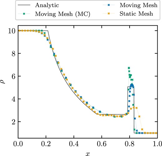
Density profile in the relativistic shocktube problem at t = 0.4. The solid line is the exact solution. The calculations corresponding to the coloured lines are listed in the legend. All simulations employ the same initial conditions and resolution. Crosses show the location of mesh cells.
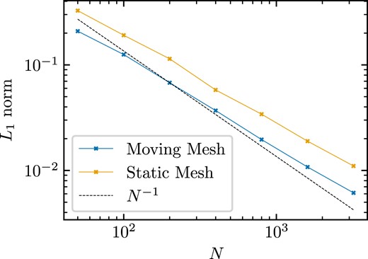
L1 norm of the density field at various resolutions for the shocktube problem at t = 0.4. The blue line corresponds to moving-mesh set-ups, while the orange line to static-mesh set-ups. The slope of the dashed line depicts first-order convergence.
APPENDIX C: COLLISION OF RELATIVISTIC BLAST WAVES
We consider the collision of two relativistic blast waves (see e.g. section 6.2.3 in Martí & Müller 2003). The initial data consist of three states, the left state (x < =0.1) where pL = 1000, the central state (0.1 < x < =0.9) where pC = 0.01 and the right state (x > 0.9) where pR = 100. Initially, the density is everywhere equal to 1 and the velocity is zero everywhere. The EOS is an ideal gas with Γ = 1.4, and we adopt outflow boundary conditions, similar to Martí & Müller (1996). We perform a moving- and a static-mesh simulation, where we initially distribute 800 equally spaced points in a domain [0,1]. Both calculations employ piecewise constant reconstruction to highlight the effect of a moving mesh in a low-order scheme. We note that the purpose of this test is to highlight the ability of a moving-mesh approach to capture the density evolution of the system with good accuracy, even when low-order schemes are considered. High-order schemes are capable of resolving the structure of the solution (see e.g. Martí & Müller 1996, for piecewise parabolic reconstruction and a considerably higher resolution than the one discussed here).
Fig.C1 shows the density profile of the system at t = 0.43, i.e. after the interaction of the two waves. We show a narrow region which includes the states produced by the collision. The blue points correspond to the moving-mesh calculation, while the orange points display the static-mesh calculation. The solid line is the exact solution based on the calculation in Martí & Müller (1996). The difference between the moving- and static-mesh calculations is very obvious. The static-mesh set-up does not resolve any structure and the states are completely smeared out. Furthermore, the position of the peak is incorrect. Considering the low order of the scheme and the low resolution, this is a reasonable result for the static mesh (see also Martí & Müller 1996). In contrast, the moving-mesh simulation is able to capture the various structures in the collision region relatively accurately. The two distinct states at different heights of the main peak can be identified, while the heights of the states are reproduced reasonably well. Furthermore, the positions of the various states in the collision region are well resolved with only a minor offset. Overall, even though the cells are initially distributed evenly in the simulation domain, the moving mesh follows the fluid motion, which enables it to accurately resolve the very narrow structures which form in this problem.
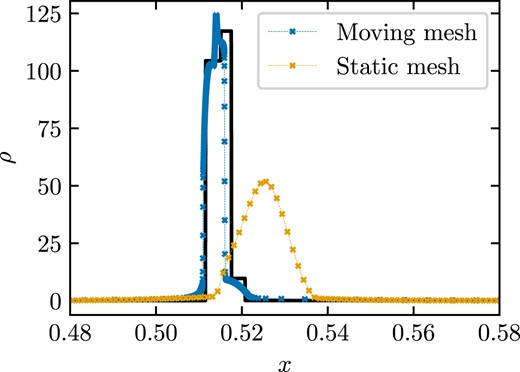
Density profile of the blast wave collision problem at t = 0.43. The solid line is the exact solution. The blue points and line correspond to a moving-mesh calculation, while the orange points and line to a static-mesh calculation with the same initial conditions and resolution. Crosses show the location of mesh cells.
APPENDIX D: NUMERICAL SET-UP
D1 BNS merger: resolution study, GW back-reaction effect, and code performance
We perform a number of additional simulations for the binary system discussed in Section 5 to investigate the effect of a number of numerical aspects. These include the hydrodynamical resolution in the simulation (i.e. the number of hydro cells), the resolution employed in the metric solver and the impact of enhancing the strength of the GW back-reaction scheme. We consider the following:
A simulation with a lower hydro resolution. We follow the procedure discussed in Section 5.1 to construct the initial hydrodynamical mesh and set mcell,0 = 2.4 × 10⁻⁶ M⊙. This results in a mesh with roughly 1.2 × 10⁶ cells with ρ > ρthr, which corresponds to about |$\approx 70~{{\ \rm per\ cent}}$| of the mass resolution of the original simulation. Other choices of the numerical set-up (e.g. the metric grid resolution) remain identical to the original simulation.
A simulation with an hydrodynamical set-up identical to the one described in Section 5.1, but the metric field equations are solved on an overlaid uniform Cartesian grid with 1933 points and a cell size of 0.533 M⊙ (i.e. the metric grid resolution is higher than in the original simulation).
An identical setup to the one discussed in Section 5.1, where we enhance the strength of the GW back-reaction scheme. This is achieved by multiplying the derivatives of the quadrupole moment entering the source terms in equations (A2)–(A3) by a factor of 2 (see Appendix A). Hence, we effectively account for the observation that the quadrupole formula may underestimate the GW signal amplitude by some 10 per cent (see e.g. Shibata, Taniguchi & Uryū 2005; Diener, Rosswog & Torsello 2022). A factor of 2 is chosen to safely bracket the potential impact.
Fig. D1 shows the GW strain amplitude for the simulation discussed in Section 5, as well as all three additional simulations presented here. We present the amplitude |$\sqrt{h_\mathrm{+}^2+h_\mathrm{x}^2}$| for all the simulations, while for case (iii) we also include the plus polarization of the GW signal, h+. We emphasize that for case (iii) we extract h+ from the quadrupole moment without including the enhancement factor of 2. This factor is only included in the quadrupole moment derivative terms in equations (A2)–(A3). As a result, all the simulations reported in Fig. D1 have comparable amplitudes. The subpanel within Fig. D1 zooms in on the first 10 ms of the post-merger phase. Like this the characteristics of the GW amplitudes are easier to read off. In all cases, the signals are shifted such that t − tmerg = 0 corresponds to the moment of merging in the respective simulation.
Comparing the simulations that have a different hydrodynamical or metric resolution to the standard set-up [i.e. cases (i) and (ii)], we find a stronger dependence on the hydrodynamical resolution, but overall good agreement with the original simulation. Reducing the hydrodynamical resolution, the stars merge ≈1.2 ms earlier compared to the standard simulation. Increasing the metric resolution has a milder effect and the stars merge ≈0.3 ms later than the original set-up10 Similarly, the GW signal in the early post-merger phase remains practically unaffected by the increase in the metric resolution and only a very mild effect can be seen in the simulation with lower hydrodynamical resolution. On longer time-scales of several 10 milliseconds, the GW signal still looks very similar in all three simulations [comparing the standard set-up, case (i) and case (ii))] and the damping times-scale is practically the same. The double-core structure persists for ≈1.5 ms less in the run with the lower hydro resolution compared to the standard set-up, while the higher metric resolution has practically no effect on when the cores merge.
Enhancing the strength of the GW back-reaction scheme [case (iii)] has a more noticeable effect on the evolution, which is expected since GWs are an important damping mechanism. The inspiral time is reduced by ≈5.4 ms. The impact of a stronger GW back-reaction in the early post-merger phase is a bit more pronounced than the effects considered in cases (i) and (ii). We note, however, that we changed the hydro resolution only within a relatively small range and thus we cannot exclude that the choice of the hydrodynamical resolution may actually have a larger effect. Furthermore, the damping time-scale of the GW emission is shorter than our standard set-up, which becomes clearly visible at late times in Fig. D1. We emphasize that the damping of the post-merger signal remains very slow and we extract a damping time-scale of τpeak ≈ 31 ms based on the model in Soultanis, Bauswein & Stergioulas (2022). In addition, we find that the two cores in the post-merger phase merge after roughly 12 ms. Hence, in the set of neutron star merger simulations discussed in this work, certain dynamical features in the post-merger phase seem to consistently persist for longer time-scales compared to simulations with other numerical schemes.
Finally, we comment on the effect of the different resolutions in the hydro scheme [case(i)] and metric solver [case (ii)] on the computational costs. arepo is written in C and parallelized for distributed memory systems with MPI. The metric solver is written in Fortran and parallelized with OpenMP. We emphasize that the numbers quoted here are only representative of specific simulations presented here. The distribution of mesh-generating points can affect how much time is required for the various operations within a time-step, e.g. for the mesh construction. As measure of the computational costs, we consider the wall clock time required for a time-step where the metric field equations are explicitly solved and a time-step where the metric fields are only extrapolated (see Section 3.1). The second value is representative of how much time is required for the various operations related to the hydrodynamical evolution and the mesh construction,11 while the difference between the two numbers captures the costs for metric-related operations (namely the metric solver and the treewalk to place metric grid points in the Voronoi hydrodynamical mesh). We extract these times as an average of the first 100,000 steps in each simulation to get representative values. We exclude time-steps where a snapshot of the full 3D simulation data is produced, which is a major I/O operation. For the standard set-up, we find that the average time-step where the metric field equations are explicitly solved takes ≈8.1 s, while extrapolating the metric fields reduces the time to ≈5.9 s. For the simulation with lower hydro resolution, these numbers are ≈5.7 s and ≈3.4 s, respectively. The metric resolution is the same in both simulations, and thus the time spend for the metric solution is roughly constant (about 2.2 s). We note that our standard set-up employs 192 cores, while the simulation with a lower hydrodynamical simulation uses 184 cores. Finally, increasing the metric grid from 1293 (standard set-up) to 1933 (case (ii)) raises the time spent on metric-related operations from ≈2.2 s to 8.2 s. Hence, considering only the time spent in the metric solver, we find that in the run with a better metric resolution it increases by a factor of ≈3.8, which indicates a very good scaling for the metric solver, since a perfect scaling would be 1933/1293 ≈ 3.35.
D2 Frequency of solving the metric field equations
In Section 3.1, we discuss how frequently we solve the metric field equations within the time integration scheme. Here, we investigate the impact of this choice to justify the approach. Focusing on the evolution of TOV stars, we perform a moving-mesh simulation with the low-resolution set-up described in Section 4.2.1, where we solve the metric field equations in every substep of the time integration. We present the maximum density evolution from this simulation in Fig. D2(a) (orange line). The blue line displays the density evolution for the original set-up where we solve the metric field equations according to the description in Section 3.1, i.e. employing an extrapolation for a subset of time-steps. We find that the frequency of solving the metric field equations has practically no impact on the evolution. Both the amplitude of the oscillation, as well as the dominant frequency, remain practically unaffected by solving the metric field equations more frequently.

Gravitational wave amplitude |$\sqrt{h_\mathrm{+}^2+h_\mathrm{x}^2}$| versus time for the simulations outlined in the legend. For the simulation with an enhanced back-reaction, the plus polarization is also shown (see the main text). A smaller panel which depicts a zoomed in version of the first 10 ms in the post-merger phase is also included. Note that h+ is shown, unlike Fig. 12 which displays |$h_\mathrm{+}^\mathrm{1.4}$|.
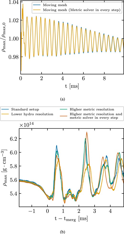
Impact of solving the metric field equations in every substep of the time integration scheme on the density evolution. Panel (a): Moving-mesh simulations of TOV stars. The blue line corresponds to the low resolution moving-mesh setup discussed in Section 4.2.1, while the orange line is the same setup where the metric fields are explicitly computed in every substep. Panel (b): Effect on BNS simulations. The original setup from Section 5 is shown in blue together with three additional calculations with lower hydro resolution (orange), higher metric resolution (green) and higher metric resolution combined with solving the field equations in every substep (red).
In addition, we evolve the standard resolution moving-mesh set-up from Section 4.2.1, but we explicitly solve the field equations in the first substep of every Runge–Kutta time-step, i.e. we call the metric solver more frequently compared to our default settings. We again find that it does not affect the overall evolution and the differences are even less visible than in Fig. D2(a).
Furthermore, we evaluate the effect of explicitly solving the metric field equations in every substep of the time integration scheme in the case of a BNS merger. We consider the set-up described in case (ii) in Appendix D1 (i.e. the metric grid resolution is 0.533 M⊙) and simulate the interval from 1.75 ms before the moment of merging up to 4.85 ms after the time of merging. The metric fields change rapidly during merging. Hence, this is arguably the most challenging interval during the simulation to accurately estimate the values of the metric fields based on extrapolation. Fig. D2(b) shows the evolution of the maximum density close to the moment of merging for four different simulations. In addition, we overplot three more simulations: the original BNS simulation discussed in Section 5 (with a lower metric resolution), as well as the set-ups with lower hydro resolution [case (i)] and higher metric resolution [case (ii)] from Appendix D1.
The set of simulations presented in Fig. D2(b) allows to judge the impact of solving the metric field equations more frequently in comparison to other numerical choices like a different hydro or metric resolution. We find that the two calculations with a metric resolution of 0.533 M⊙ progress rather similarly, but solving the metric field equations more frequently does have a recognizable impact on the maximum density evolution. This result suggests that BNS simulations can benefit up to some extent from solving the metric field equations more frequently, at least during the merger stage. However, we note that the differences are smaller than those that one obtains from a change of the hydro resolution by 30 per cent (considering the number of cells resolving stellar matter). This justifies a practical approach where saving computational resources by calling the metric solver less often can be used for a better resolution.
