


ABSTRACT
Subsonic turbulence plays a major role in determining properties of the intracluster medium (ICM). We introduce a new meshless finite mass (MFM) implementation in OpenGadget3 and apply it to this specific problem. To this end, we present a set of test cases to validate our implementation of the MFM framework in our code. These include but are not limited to: the soundwave and Kepler disc as smooth situations to probe the stability, a Rayleigh–Taylor and Kelvin–Helmholtz instability as popular mixing instabilities, a blob test as more complex example including both mixing and shocks, shock tubes with various Mach numbers, a Sedov blast wave, different tests including self-gravity such as gravitational freefall, a hydrostatic sphere, the Zeldovich-pancake, and a 1015 M⊙ galaxy cluster as cosmological application. Advantages over smoothed particle hydrodynamics (SPH) include increased mixing and a better convergence behaviour. We demonstrate that the MFM-solver is robust, also in a cosmological context. We show evidence that the solver preforms extraordinarily well when applied to decaying subsonic turbulence, a problem very difficult to handle for many methods. MFM captures the expected velocity power spectrum with high accuracy and shows a good convergence behaviour. Using MFM or SPH within OpenGadget3 leads to a comparable decay in turbulent energy due to numerical dissipation. When studying the energy decay for different initial turbulent energy fractions, we find that MFM performs well down to Mach numbers |$\mathcal {M}\approx 0.01$|. Finally, we show how important the slope limiter and the energy-entropy switch are to control the behaviour and the evolution of the fluids.
1 INTRODUCTION
Turbulence plays a key role in a variety of astrophysical systems at all scales, ranging from stellar structure, star-formation in the interstellar medium (ISM) all the way up to the instracluster medium (ICM). It leads to enhanced small-scale mixing, and contributes to the global pressure of a system. While being mostly supersonic in the ISM, turbulence is mainly subsonic in the ICM (compare, e.g. Schuecker et al. 2004, for observations on the Coma cluster). A theoretical framework for subsonic turbulence has been provided by Kolmogorov (1941), assuming isotropy. Simulations are an essential tool to better understand physical properties of astrophysical turbulence as well as its influence on local observables such as star formation in the ISM or its contribution to heating in the ICM.
Historically, there exist different methods to solve the hydrodynamical equations in comoving/cosmological context. Hereby, one has the option to discretize the hydrodynamic equations by mass or volume. The former leads to the concept of ‘Lagrangian’ (particle based) codes and the concept of smoothed particle hydrodynamics (SPH), and the more recent meshless finite mass (MFM) and meshless finite volume (MFV). The latter gives rise to the concept of ‘Eulerian’ (grid based) codes and the Godunov finite volume approach.
Popular SPH codes include Gadget in the different versions including Gadget-1 (Springel, Yoshida & White 2001), Gadget-2 (Springel 2005), and Gadget-4 (Springel et al. 2021), phantom (Lodato & Price 2010; Price et al. 2018), and gasoline (Wadsley, Stadel & Quinn 2004; Wadsley, Keller & Quinn 2017). An improved SPH scheme with non-standard enhancements has been implemented in magma2 (Rosswog 2020). MFM has been implemented in e.g. gizmo (Hopkins 2015), gandalf (Hubber, Rosotti & Booth 2018), Gadget-3 (Steinwandel et al. 2020), and pkdgrav-3 (Alonso Asensio et al. 2023).
Mesh codes exist in two flavours: either as a stationary mesh, possibly with adaptive mesh refinement, as implemented e.g. in zeus (Stone & Norman 1992), tvd (Ryu et al. 1993, 1998), enzo (Bryan et al. 1995, 2014), flash (Fryxell et al. 2000), ramses (Teyssier 2002), athena (Stone et al. 2008), and athena++ (Stone et al. 2020) or as a moving mesh as in Arepo (Springel 2010; Weinberger, Springel & Pakmor 2020), and shadowfax (Vandenbroucke & De Rijcke 2016). The latter have the advantage of being Pseudo-Lagrangian. While mesh codes as well as MFM employ a Godunov-method and calculate fluxes between neighbours (Godunov 1959), SPH directly retrieves the hydrodynamical fluid vectors from the kernel density estimation that is obtained by adopting a weighted sum over a certain (typically non-constant) number of neighbours.
All of them can be used for computations of turbulence, with earlier calculations primarily carried out in the supersonic regime, relevant in the ISM for regulating star formation. Many results have been obtained assuming driven turbulence in which an energy input at large scales is provided during the whole simulation. In contrast to driven turbulence, we expect decaying turbulence to be present in galaxy clusters. Turbulence is injected at large scales for example due to collapse of large scale structure and subsequent merger activity (Roettiger & Burns 1999; Subramanian, Shukurov & Haugen 2006), after which, it energy is transported down to the smaller scales (‘turbulent cascade’) on which it is dissipated (generally below the resolution scale of any given code).
In the series of papers by Federrath, Klessen & Schmidt (2008, 2009) and Federrath et al. (2010), they have used a stationary grid code to calculate turbulent boxes with driven turbulence. They found that the choice of the driving scheme plays an important role in determining properties of the resulting turbulence, leading to significant differences in the density statistics. Their results suggest a different mixture of driving mechanisms for different star-forming regions. Overall, they found good agreement with observations as well as other results, independent of the driving mechanism employed. More recently, Federrath et al. (2021) increased the resolution to even resolve the sonic scale, starting from supersonic turbulence with a resolution of ∼10 0003 cells.
Kitsionas et al. (2009) and Price & Federrath (2010) also compared the performance of different implementations of SPH and hydro schemes with a stationary mesh, and find good agreement between these two methods at high Mach numbers. Mesh codes are more efficient to obtain volumetric statistics such as the power spectrum, while SPH recovers the high-density tail better due to automatically adapting the resolution.
While all these methods work well in the supersonic turbulent regime, they have problems dealing with subsonic turbulence. Going to smaller Mach numbers (|$\mathcal {M}$|), Padoan et al. (2007) showed that SPH performs sub-optimum when compared to finite volume methods. Based on this work, Bauer & Springel (2012) studied the capabilities of SPH for subsonic turbulence at |$\mathcal {M}=0.3$|. They found that classic (vanilla) SPH fails in reproducing the expected velocity power spectrum as well as the dissipation range. Reasons are mainly the artificial viscosity scheme used and velocity noise introduced by the kernel. These results raised the general question of whether SPH can deal with subsonic turbulence to begin with.
An answer has been provided by Price (2012) who showed that these limitations are not intrinsic to SPH, but rather a consequence of some SPH set-ups adopted to study subsonic turbulence. In contrast to what previous studies reported, SPH can capture the expected power spectrum by using more modern formulations of SPH that are able to reduce artificial viscosity in subsonic regimes.
The role of subsonic turbulence in galaxy clusters has been analysed both from observational and theoretical perspectives. Simulations of turbulence in the ICM have been carried out mostly using grid codes (Iapichino & Niemeyer 2008; Vazza et al. 2009; Iapichino, Federrath & Klessen 2017; Vazza et al. 2018; Mohapatra, Federrath & Sharma 2021; Mohapatra et al. 2022). Miniati (2014, 2015) found a lack of turbulent energy at small scales depending on the refinement technique. In addition, they discussed the importance of microphysics for the evolution of turbulence. A possible improvement for modelling turbulence has been presented by Maier et al. (2009) combining AMR with large eddy simulations. Simulations by Dolag et al. (2005b) have shown that also SPH can model turbulence in galaxy clusters when properly reducing artificial viscosity.
In addition to the impact on gas dynamics, turbulence is responsible for amplifying magnetic fields through a turbulent dynamo. Simulations by Schekochihin et al. (2001, 2004) and Steinwandel et al. (2022) have focused on this turbulent dynamo, analysing its growth. Another work of Kritsuk et al. (2020) has focused again on turbulent boxes with stochastic forcing, comparing different hydrodynamical methods and finding reasonably good convergence but significant differences in computational costs.
More recently, Sayers et al. (2021) have compared simulated clusters to observed ones. Especially, there should be a difference depending on the dynamical state, with more relaxed clusters showing less turbulence. Simulations, however, do not always find such a difference. Thus, it is important to accurately capture the turbulent cascade and the decay in turbulent energy. While the latter would require including additional microphysics such as viscosity, the former also depends on the hydro scheme.
We use MFM as an alternative, newer method to the aforementioned ones to study subsonic turbulence. MFM combines ideas of SPH with those of a moving mesh and thus aims at solving several of their individual issues. The development of MFM goes back to first ideas presented by Vila (1999) and Godunov SPH (Inutsuka 2002; Cha & Whitworth 2003), which was still unstable, and to a meshless finite element method suggested by Idelsohn et al. (2003), until the nowadays used version first formulated by Lanson & Vila (2008a, b). We present a new implementation in the Gadget derivative OpenGadget3, originally based on that in the code gandalf, where the skeleton of the MFM implementation has been originally taken from their code-base and then adjusted. Several extensions allow its use in cosmological simulations compared to the implementation in gandalf that is focused on star and planet formation. This allows for a stable baseline framework for applications on scales of star and planet formation that we extend into the cosmological integration framework of OpenGadget3, which is a re-base of Gadget-2 with the ability to be compiled with C++ compilers, and making vast use of templating. It comes with modules containing state-of-the-art physics and sub-resolution models, as for instance: self-interacting dark matter (Fischer et al. 2022), magnetohydrodyanamics (MHD) (Dolag & Stasyszyn 2009; Stasyszyn, Dolag & Beck 2013), thermal conduction (Arth et al. 2014), cosmic rays (Böss et al. 2023), star formation and stellar/blackhole feedback according to the Magneticum-model (Springel & Hernquist 2003; Tornatore et al. 2003, 2004, 2007; Hirschmann et al. 2014; Dolag 2015; Steinborn et al. 2015), or with the MUPPI (MUlti Phase Particle Integrator) extension for non-equilibrium star formation (Murante et al. 2010, 2015; Valentini et al. 2017, 2020). These extensions are so far coupled only to the SPH hydro-solver. Further work will be required to couple them also to MFM.
To make use of modern computer architectures, OpenGadget3 includes a hybrid MPI-OpenMP parallelization. In addition, calculations of gravity, density, SPH hydro-force, and thermal conduction, can be carried out on GPUs. These modules requiring most of the runtime (Ragagnin et al. 2020) GPU offloading can be useful for some applications, leading to a speed up by a factor of a few (2–4, depending on the exact application). The long-term goal is to have a fully publicly available updated Gadget version for OpenMP and OpenACC.
Before the introduction of this paper, the code was solving the hydrodynamical equations using modern SPH as formulated by Springel & Hernquist (2002), including modern time-dependent artificial viscosity (Beck et al. 2016a) and conduction (Price 2008). With the new implementation of MFM as a modern meshless method, we can combine advantages both of this method and efforts previously made to optimize the pre-existing code base. This also involves a treatment in order to evolve strong shocks for which we need the time-step limiter to be non-local which is ensured by a wakeup scheme (Saitoh & Makino 2009; Pakmor 2010; Pakmor et al. 2012). OpenGadget3 closely follows the implementation described by Beck et al. (2016a).
A main goal of this paper is to use MFM to study decaying, subsonic turbulence, as present in galaxy clusters. To this end, we present a new implementation in the cosmological simulation code OpenGadget3 as an alternative hydro-solver to the currently implemented SPH.
This paper is structured as follows. We first describe the codebase of OpenGadget3 including its SPH implementation in Section 2. We continue with a brief overview on MFM and a description of our MFM implementation in Section 3. In Section 4, we use a suite of test cases, each probing specific aspects and properties of the code, to validate the performance of our MFM implementation. All settings are kept exactly the same between test cases, independent of the individual test case, without further tuning. We continue with an analysis of decaying subsonic turbulence with our new implementation presented in Section 4.6. In all cases, comparisons between different codes and methods are provided, including MFM and SPH in OpenGadget3, MFM in gizmo and a moving and stationary mesh in the publicly available Arepo version. We analyse the effect of specific numerical parameters in Section 4.8. Our main findings are discussed in Section 5.
Additional material such as the formulation of the slope-limiters and a comparison of the Riemann solvers implemented are presented in Appendices A and B, respectively.
2 OPENGADGET3–BACKBONE
Solving the system of differential equations describing the evolution of the gas requires discretizing them. In the temporal dimension, a sufficiently small time-step Δt is introduced. The spatial discretisation can be obtained using various different approaches. In OpenGadget3, hydrodynamics is discretized either using smoothed particle hydrodynamics (SPH) or with the newly implemented MFM. Gravity is solved by a TreePM method.
2.1 Integrator and time-stepping
For the time integration, we employ a Leapfrog scheme in kick–drift–kick (KDK) form to achieve second order accuracy (compare e.g. Hernquist & Katz 1989) in the implementation following Verlet (1967) and Springel (2005).
Starting from values at time-step number n, velocities |${\boldsymbol v}$| are updated in a first half-step kick. It is followed by drifting the positions |${\boldsymbol r}$|, and another, second half-step kick
The acceleration |${\boldsymbol a}^{\tilde{n}}={\boldsymbol a}_{\text{hydro}}^{\tilde{n}}+{\boldsymbol a}_{\text{grav}}^{n}$| consists of hydrodynamical accelerations |${\boldsymbol a}_{\text{hydro}}$| and gravitational accelerations |${\boldsymbol a}_{\text{grav}}$|. Following the operator splitting approach, they are calculated separately. Gravity and hydrodynamical accelerations are evaluated between the drift and the second half kick. Gravitational interactions depend only on the position, and can thus be calculated at time-step n. While for traditional SPH entropy does not change, such that also a calculation of the hydrodynamical forces at time-step n is possible, there is an evolution of entropy and also a velocity dependence for the viscous terms of modern SPH. Thus, we use predicted values based on the changes calculated during the previous time-step, updated at the drift. The dependence of the predicted variables is indicated by |$\tilde{n}$|.
For SPH, the entropic function
is integrated in two half-steps at the kicks
While traditional SPH is conserving entropy, it is allowed to change in the modern SPH implementation due to e.g. artificial viscosity and conductivity.
OpenGadget3 uses hierarchical time-stepping to ensure synchronization, while allowing adaptive time-steps, depending on different time-step limiters such as a Courant-like time-step criterion
with maximum signal velocity over the neighbours cmax, i, scale factor a, smoothing length hi, and free parameter CCourant, as described by Springel (2005). Time-steps are chosen as the largest time-step that fulfills |$\Delta t_i = 2^{-n}\Delta t_{\text{global}}\le \Delta t_i^{\text{Courant}}$| with time bin |$n\in \mathbb {N}_0$|.
Accelerations are calculated only for active particles, which are in synchronization with the current time-step, while they are not modified for particles located on a smaller time bin, corresponding to larger time-steps.
For strong shocks, large differences can occur between the time-steps of close-by particles. This is avoided by a wake-up scheme, described in more detail by Pakmor (2010), Pakmor et al. (2012), and Beck et al. (2016a). OpenGadget3 uses a criterion based on the signal velocity. If for any neighbour j, the signal velocity varies strongly cmax, i > fwcj with tolerance factor fw = 3, wake-up is triggered. In this case, the particle is considered active and moved to a shorter time-step, such that synchronization is still ensured.
While this scheme will break conservation, it works reasonably well and avoids numerical errors in strong shocks.
2.2 Gravity Solver–TreePM
The accurate treatment of gravity is of great importance for cosmological simulations (Springel 2010). In principle, it can be solved accurately by a direct summation, which is, however, computationally expensive (|$\mathcal {O}(N^2)$|). Instead, we follow the much more efficient combined Oct-Tree-Particle Mesh (PM) approach (Xu 1995; Bode, Ostriker & Xu 2000; Springel 2005, 2010; Springel et al. 2021). OpenGadget3 mainly follows the implementation in Gadget-2, which has been extensively described by Springel (2005). In the following, we briefly review the main concept. The potential is split into short-range and long-range contributions. Short-range forces are calculated following the oct-tree algorithm, while long-range forces are calculated using a particle mesh. The idea of a tree algorithm has been proposed by Appel (1985) and Barnes & Hut (1986). Nodes of an oct-tree are constructed by splitting the domain into a sequence of cubes. Force-contributions of nodes satisfying an opening angle criterion are calculated. For numerical reasons to keep the equation linear with respect to adding and removing particles from nodes, only the monopole contributions are taken into account. The implementation in gGadget has been described by Springel et al. (2001). The total gravitational acceleration of particle i from other nodes/particles j with mass mj at location |${\boldsymbol r}_{ij}$| relative to particle i and with (gravitational) softening length ϵj is given by
with total number of particles and nodes Ntot. Corr is a correction term, taking into account the softening. G is the gravitational constant. For the particle mesh (Eastwood & Hockney 1974), all particles are assigned to grid-cells, such that a discrete Fourier-transformation can be calculated, with the gravitational potential Φk in Fourier space at wavenumber k being calculated as
Corrections for small-range truncation as well as periodic boundaries are applied by multiplications in Fourier space. The gravitational potential in real space is calculated as inverse Fourier-transform, and is interpolated to the original particle positions to finally obtain gravitational accelerations. OpenGadget3 uses the more modern FFTW3 (‘Fastest Fourier Transform in the West’) library (Frigo & Johnson 2005) instead of FFTW2 for the implementation of the Fourier transform.
2.3 Hydrodynamical Solver–SPH
For smoothed particle hydrodynamics (SPH), the domain is decomposed into a finite number of ‘particles’. The physical quantities at each point are represented by contributions of close-by (neighbouring) particles weighted by a kernel |$\mathcal {W}_i(r_i,h_i)$|, depending on the distance ri from particle i, and its smoothing length hi. The kernel has to be continuous, radially symmetric, have compact support, and fulfill the limit |$\lim _{h\rightarrow 0}\mathcal {W}= \delta$|, but otherwise can be chosen arbitrarily. OpenGadget3 offers the choice between different commonly used kernels, including a cubic spline (Monaghan & Lattanzio 1985), quintic spline (Morris 1996), or a Wendland C2/C4/C6 kernel (Wendland 1995; Dehnen & Aly 2012). The effective volume of each particle is well approximated by |$V_i^{-1}=\mathcal {W}(r_{i})$|, such that the density follows as
summing over the neighbouring particles (Ngb). We allow for adaptive smoothing, automatically increasing resolution in high-density regions compared to low-density ones. Smoothing length and effective neighbour number NNgb are related to the density via
with mean neighbour mass |$\bar{m}$|. As equations (10) and (11) are coupled for fixed neighbour number, one solves for smoothing length and density iteratively via finding roots. Quantities other than the density, labelled with X, are approximated via
Different formulations of the hydrodynamical acceleration can be derived. In OpenGadget3 the fully conservative formulation for the hydrodynamical acceleration (Springel & Hernquist 2002)
is utilized. Instead of calculating gradients of physical quantities, all spatial derivatives are expressed by gradients of the kernel function. Traditional SPH has problems dealing with shocks, as well as reproducing mixing instabilities (Morris 1996; Agertz et al. 2007). These issues can be resolved by including artificial viscosity and conductivity. In OpenGadget3, time and spatial dependent artificial viscosity (Beck et al. 2016a) and artificial conductivity (Price 2008) are utilized, minimizing their impact in regions where they are not desired.
3 MESHLESS FINITE MASS
As a second, newly implemented option, the hydrodynamical equations can be discretized and solved following the MFM approach. This method conceptually combines SPH with a moving mesh, calculating fluxes between neighbouring particles in a scheme otherwise similar to SPH, including weighting by a kernel. Thus, it is combining advantages of both methods. In contrast to SPH, the domain associated to a particle is not spherical, but rather corresponds to a smoothed Voronoi tesselation (Hopkins 2015).
3.1 Basic hydrodynamical equations
The evolution of any ideal fluid is described by three main equations. Mass conservation leads to the continuity equation. The second equation is an equation of motion (Euler’s equation), corresponding to Newton’s second law. Energy conservation is ensured by the first law of thermodynamics. Within an inertial frame of reference, all these equations can be combined into
with outer product ⊗ and, for pure hydrodynamics, field vector |${\boldsymbol U}=(\rho ,\rho {\boldsymbol v},\rho e)$|, flux |$\bf{F}=(\rho {\boldsymbol v}, \rho {\boldsymbol v}\otimes {\boldsymbol v} + P{1}, \left(\rho e + P\right){\boldsymbol v})$| and vanishing source terms |${\boldsymbol S}={\boldsymbol 0}$|.
In total, equation (15) provides 5 constraints for 6 variables: fluid density ρ, energy density e, pressure P, and the three components of the velocity |${\boldsymbol v}$|. The missing constraint is provided by an equation of state, connecting the pressure to the internal energy density u. For an ideal gas, it takes the form
where the adiabatic index γ amounts to 5/3 if the gas is monoatomic.
3.1.1 Equations in an expanding universe
In a cosmological context, the expansion of the universe has to be taken into account. One possibility is to rewrite equation (15) for a universe with scale factor a, accounting for these effects, as realized e.g. in Gadget-1
In OpenGadget3, we follow a different approach, and do calculations using the so called supercomoving coordinates, as first introduced by Martel & Shapiro (1998). Code units (denoted by subscript c) are related to physical units (p) via
such that equation (15) keeps the same form when written in code units except for an additional contribution in the energy and momentum evolution due to the Hubble expansion. As we use peculiar velocities, the explicit dependence on the Hubble flow for momentum is absorbed into the choice of units.
3.2 MFM discretization
Mathematically, equation (15) is discretized by multiplying by a partition function
where |$\mathcal {W}_k=\mathcal {W}(\left|r-r_k\right|,h_k)$| and integrating over the volume. A more detailed derivation has been provided by Lanson & Vila (2008a) and Gaburov & Nitadori (2011). In this paper, we only focus on the key results relevant for the implementation. For every particle i, changes in the quantities |${\boldsymbol U}_i=(\rho _i, \rho _i v_i, \rho _ie_i)$| are given by source terms |${\boldsymbol S}_i$|, which vanish for pure hydrodynamics, and pairwise fluxes |$\bf{F}_{ij}$| with the neighbours j
Calculating pairwise fluxes automatically ensures mass, momentum and energy conservation. The effective interface area |${\boldsymbol A}_{ij}^{\text{eff}}$| depends on the partition function and effective volume Vi,
where
with Einstein summation convention over β in equation (28). The matrix |$\bf{B}$| is chosen in order to be second order accurate (Lanson & Vila 2008a)
Also, the effective volume depends on the integrated partition function and can be expressed in terms of the number density ni:
For highly unisotropic particle arrangements, the matrix |$\bf{E}$| can become ill-conditioned, preventing an accurate numerical matrix inversion. As described by Hopkins (2015), we use the condition number |$N_{\text{cond},i}=N_{\text{dimensions}}^{-1}\sqrt{\left|\left|\bf{E}_i^{-1}\right|\right|\left|\left|\bf{E}_i\right|\right|}$| as measure of how well conditioned the matrix is. For Ncond, i > 100 gradients are calculated only first order in an SPH-like way.
Most importantly, no tessellation has to be calculated explicitly as it would be necessary for a moving mesh, but an SPH-like neighbour search is used, drastically reducing the computational costs compared to the mesh reconstruction.
In contrast to SPH, for which the mass density is estimated according to equation (11), for MFM, the number density ni is estimated together with the smoothing length in an iterative process, solving
Also for MFM, NNgb corresponds to the effective neighbour number.
The flux in equation (26) is calculated numerically using a Riemann solver, where we use an exact Riemann solver, following the implementation by Toro (2009) with a tolerance of 10−4, and a maximum of 8 iterations. Alternatively, we implemented the Riemann-solver that provides an exact solution to the linearized system of equations (Roe-solver; Roe 1981), as well as the two most common flavours of a Harten–Lax–van–Leer solver (HLL) and HLLC (Toro 2009). For all these, the exact Riemann solver is used as fallback in case the faster approximate solver fails. The effect of the choice of the solver is discussed in more detail in Appendix B.
The Riemann solver requires knowledge about velocity, density, and pressure values at the interfaces, summarized in the primitive fluid vector
In principle, values at the particle centre can be used directly, following a zeroth order interpolation. While such a scheme would be stable, it is only first order accurate and very diffusive (Godunov 1959; Barth & Jespersen 1989). To this end, we follow a two-step approach, as illustrated in Fig. 1, similar to what is usually done for grid-based methods and in other MFM implementations.
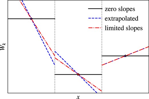
Sketch of extrapolation from central particle/cell values to face values. Using the central values corresponds to a zeroth order interpolation, leading to a first order scheme (black solid lines). It can be extended to be second order by extrapolating using a slope defined by neighbouring particles/cells (blue dashed line), which however can lead to over/undershooting at the faces (see left face) or even negative densities/pressures (see right face). This issue can be solved by limiting the slopes using different procedures (red dash–dot line). See the text for further details.
In a first step, gradients of the primitive fluid vector are calculated using a second-order accurate matrix gradient estimator
The position and velocity of the face is estimated via
where we set
to be second order accurate instead of si = 1/2 for a first-order accurate interpolation.
By choosing the reference frame corresponding to the rest frame of the interface, the scheme becomes Lagrangian. In MFM, also the boundaries are assumed to deform in a Lagrangian way, eliminating mass fluxes between neighbours. As the actual face velocity and deformation does not exactly correspond to the one assumed during a time-step, second order errors are introduced (Hopkins 2015). An alternative is allowing for mass fluxes using the MFV method, which, however, also is only second order accurate. In addition, it has been shown that MFV can run into problems by draining the mass for particles accelerated into low-density environments in cosmological simulations (Alonso Asensio et al. 2023). For this reason, we do not use this scheme here but focus on the MFM method. An additional advantage of MFM and finite volume schemes in general over SPH is that no additional dissipation terms are necessary.
The face-values are extrapolated according to
To avoid over or undershooting or even unphysical, negative densities, or pressures when strong gradients are present in the fluid, these gradients are reduced by a factor ∇Wi, k → αi, k∇Wi, k, 0 ≤ αi, k ≤ 1 in a second step in the face interpolation where αi, k can be different for each particle i and component k. We implement different options for such a slope-limiter, including a total variation diminishing (TVD) one (Duffell & MacFadyen 2011), the one from Arepo (Springel 2010) originally presented by Barth & Jespersen (1989), the scalar limiter from the gandalf code (Hubber et al. 2018), and the one used in the gizmo code (Hopkins 2015), described further in Appendix A. In addition, the pairwise limiter according to the gizmo code can be used.
In a third, final step the Riemann solver is used to calculate fluxes, which can then be converted to hydrodynamical acceleration and energy changes1. All these steps are only applied to particles which currently reside in an active time bin. While this workflow is computationally convenient, it makes the scheme less exact, as old gradients are used for the flux calculation. Nevertheless, the scheme still performs accurate enough in practical applications, as also argued by Hopkins (2015).
In addition, in our implementation fluxes are updated only for the active particle, which breaks conservation. This could be improved by updating fluxes for both particles and only considering neighbours on lower time bins. As we found no significant disadvantage for practical applications, we kept the computationally more convenient version.
3.3 Energy-entropy switch
While the Riemann solver outputs total energy changes, the rest of the code requires internal energies. Total energy itself is never used in the code. The total energy change can straightforwardly be converted into internal energy change starting from equation (26) of Gaburov & Nitadori (2011), rewriting it as a difference equation, as we have small, but finite time-steps
The velocity change can be calculated directly from the momentum change returned by the Riemann solver, as for MFM, the mass is kept constant. Thus, both time derivatives of total energy and velocity can be obtained from the Riemann solver output. We introduce the additional term |$\frac{1}{2}\left(\frac{\text{d}{\boldsymbol v}}{\text{d}t}\right)^{n}\Delta t^n$| in the bracket, which is a second order correction and improves the accuracy in the discretized equation, which is a result of discrete time-steps. While this transformation from total to internal energy does not conserve total energy to machine precision, it increases the precision in the evolution of the internal energy itself. For very cold flows, the internal energy evolution is still dominated by numerical errors. This is avoided by assuming purely adiabatic changes in these rare cases. We follow the idea of the implementation in the gizmo code, where the switch is only active for specific test problems such as the Zeldovich pancake. If active, internal energy
is compared to potential and/or kinetic energy
If the internal energy is small enough compared to other energy contributions
in physical units, the new internal energy for particle i is instead calculated assuming adiabatic expansion or contraction. The parameters α1/2 have to be tuned to only affect the evolution of particles where necessary. We provide a comparison between different values in Section 4.8.2.
The internal energy is updated similarly to the entropy for SPH in two half-steps at the kicks, following a second order time integration similar to the entropy in SPH
For cosmological simulations, additional adiabatic contributions due to the Hubble flow are added.
3.4 Switching between SPH and MFM in OpenGadget3
To substitute SPH with MFM, the general code-structure does not have to be altered. Mainly, the SPH specific force calculation has to be replaced by the three steps of the MFM calculation, consisting of gradient calculations, slope-limiting, and the actual flux calculation. As the Riemann solver both requires and outputs physical quantities, while the rest of the code deals with code units, these units have to be converted according to equations (20) to (24) just before the flux calculation. At all places, where results of that calculation, including the hydrodynamical acceleration, are used, they first have to be converted back to physical units.
Also, MFM calculates internal energy changes following the output of the Riemann solver, while in SPH the entropy is evolved.
3.5 Differences to previous implementations of MFM
While the general concept of MFM with respect to the implementations introduced in gizmo and gandalf stays the same, there are several differences compared to these previously made implementations. Our implementation is based on the one in gandalf, which is originally intended to be well suited for star and planet formation. We expand this implementation by including comoving integration and other extensions such as an energy-entropy switch to be used for cosmological applications. In addition, we change the time integration scheme from a second-order accurate MUSCL-Hancock to a second-order accurate Leapfrog KDK, consistent with SPH in OpenGadget3.
The main difference of OpenGadget3 compared to gizmo is that fluxes are by default calculated using an iterative, exact Riemann solver compared to an approximate HLLC Riemann solver used in gizmo, with an exact Riemann solver only used as fallback.
In comparison to pkdgrav-3 (Alonso Asensio et al. 2023), the energy-entropy switch and the implementation of how to deal with anisotropic particle distributions is different and more similar to gizmo.
In addition, there are a few minor differences such as the second-order correction in equation (42). We also made the pairwise limiter Lagrangian, as described in Appendix A, which was independently done also in pkdgrav-3. The convergence of the density calculation is slightly different between the codes. We follow the same implementation as for SPH in OpenGadget3, just replacing the mass density by the number density. Finally, our implementation employs a hybrid MPI-OpenMP parallelization as done for other modules of OpenGadget3.
4 TEST CASES
We use several test cases to probe the ability of the different hydro-methods to accurately follow gas evolution. Only few tests have an analytical solution, including soundwaves and different shocks. Also a set of MHD waves with analytical solution has been presented by Berlok (2022), which could be used for tests of later MHD extensions. Many other tests can be used for a more qualitative analysis. All of them explore specific numerical aspects important for cosmological simulations.
We use these tests to compare our new MFM implementation in OpenGadget3 to SPH in OpenGadget3, MFM in the public gizmo2 version and the publicly available version of the moving mesh code Arepo3.
4.1 Settings
We aim for a fair comparison of the different codes throughout the paper but adopt a general setting for slope limiters, Riemann-solvers (MFM) as well as the artificial diffusion terms (SPH) that one would adopt in cosmological simulations. While this leads to overall good performance of all solvers on almost all test cases, there are a few test problems (e.g. the square test in Section 4.3.3) for which, this is not working ideal and we will discuss this in detail in the remainder of the paper. If not otherwise mentioned, we assume an ideal gas with γ = 5/3 and all code operate on adaptive time-steps for all tests (i.e. we never force a small constant time-step to improve the accuracy of the results).
MFM is used with a cubic spline kernel and 32 (24) neighbours in 3d (2d). The slope limiter from gizmo in combination with their pairwise limiter, both as presented in Appendix A, is used. Consistent settings are chosen between OpenGadget3 and gizmo. For SPH, a Wendland C6 kernel, including bias correction (Dehnen & Aly 2012), with 295 (64) neighbours in 3d (2d) is used. The modern time-dependent artificial viscosity scheme of Beck et al. (2016a) and artificial conductivity (Price 2008) are included. For Arepo, we use additional mesh regularization based on the centre of mass, and the ‘roundness’ of the cells. An overview of all settings is made publicly available.4 If not otherwise stated, the initial conditions (ICs) are created with equal particle masses. In most cases, particles are arranged in a (perturbed) regular grid in order to reduce noise introduced by the initial particle distribution.
4.2 Stability
4.2.1 Soundwave
As a first test, we adopt a sinusodial soundwave with density ρ = 1 and small perturbation amplitude Δρ = 10−4 in a box of length 1 in x-direction and 0.75 in y/z-direction. The particles are arranged in a perturbed hexagonal close packed (hpc) grid with varying resolution. The number of particles is ranging from 643 · 0.752 up to 1283 · 0.752. In the following, we will define the resolution by the number of particles per unit-length in x-direction. We adopt a wavenumber k = 2π and a speed of sound of cs = 2/3. For this test, there is an analytic solution ρ(x, t) = ρ0 + Δρsin (k(x + cst)), which makes this test well suited to perform a convergence analysis. For this purpose, we measure the L1 error norm |$\frac{1}{N_{\text{tot}}}\sum _i^{N_\text{tot}}\left|\rho _i-\rho (x,t)\right|$|, shown in Fig. 2.
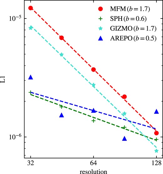
L1 norm for the soundwave at different resolutions. The order of convergence b is obtained from a fit. While MFM in both implementations shows between first and second order convergence, SPH and the moving mesh have a convergence even below first order.
All methods are able to evolve the soundwave, while the accuracy as well as the precise convergence behaviour differ among the codes. We observe a similar convergence between the MFM implementation in gizmo and OpenGadget3 being between first and second order. While theoretically second order convergence would be expected, the slope-limiter reduces the order of convergence, as discussed by Alonso Asensio et al. (2023). The convergence for SPH in OpenGadget3 and the Arepo code are similar, but even below first order. For Arepo, the main reasons for this low-order convergence are the mesh regularization, which introduces small numerical noise, and the fact that faces which contribute by less than 10−5 to the total face area are neglected (R. Pakmor, 2023 private communication). The convergence can be improved fixing these two points, as shown in Appendix C, leading to a similar convergence as for MFM much closer to second order. Nevertheless, these changes would make the code more unstable in cosmological simulations.
In order to get a more detailed analysis, we split the error between errors in the position, in the amplitude, and scatter as shown in Fig. 3.
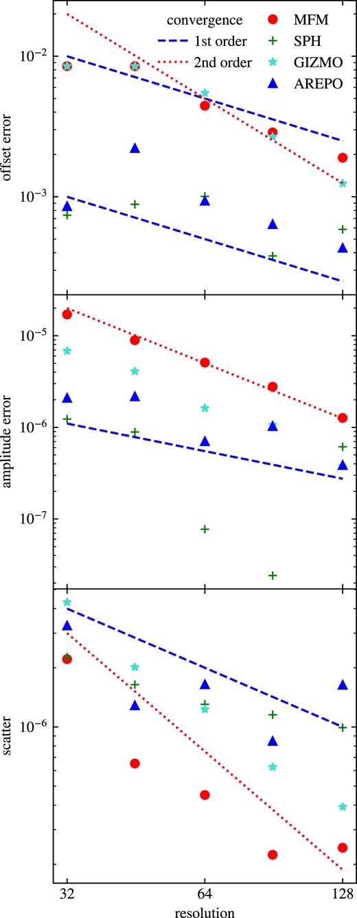
Offset-, amplitude- and scatter-errors of the density of a soundwave at |$t=\frac{2}{c_s}$| calculated with MFM and SPH in OpenGadget3, MFM in gizmo and a moving mesh in Arepo at different resolutions. The scatter converges second order for all methods, while other errors show different convergence behaviour. MFM shows between first and second order convergence for all error-components.
A sinusodial soundwave is fit to the density distribution, such that the offset and amplitude differences to the expected wave are obtained. The remaining deviations, mostly being scatter, are then quantified by an L1-norm.
Deviations from the expected sound speed are related to dispersion errors, and will lead to an offset compared to the analytical solution. This offset error is shown in the upper panel. We observe for MFM in both implementation the convergence to be between first and second order, consistent between both codes. For SPH and Arepo, the overall error is roughly one order of magnitude smaller at the lowest resolution, but having a convergence even worse than first order. For SPH, this trend can be explained by low-order errors, which are prominent for traditional SPH, and still partly left for modern SPH.
The error in the amplitude, shown in the middle panel, is related to numerical diffusion. As we see also in other tests, the Riemannn solver and the slope-limiter introduce numerical diffusivity for MFM, which thus has the largest error. Differences between the different MFM implementations can be explained by different Riemann solvers used. SPH and Arepo show much lower errors. The convergence behaviour, however, is again better for MFM compared to the other methods. In both implementations, it is roughly second order, while for the other methods, it appears to be approximately first order.
Finally, it is worth to note that the resulting soundwave does not have perfect sinusodial shape but shows scatter in the amplitude. This is mainly a result of the smoothing length/density iteration and the threshold chosen for the value to be taken as converged. We quantify this error by the L1 error norm, shown in the bottom panel of Fig. 3. All methods show roughly second order convergence, while the amplitude of the error is different. Differences between MFM and SPH in OpenGadget3 can be explained by the different kernel used, while other codes have differences in the iteration and treat parameters for convergence slightly differently. The large error for Arepo, even at higher resolution, makes the values for the other errors more uncertain. In addition to the errors already mentioned, the soundwave deforms and steepens up due to non-linear terms in the evolution. This non-linearity will lead to an additional small but constant term in the scatter error in the bottom panel of Fig. 3. A reduction could be achieved by reducing the amplitude, which would also make scatter errors be more significant or the convergence more expensive. As non-linear contribution are expected to become important when L1 ≈ (Δρ/ρ)2 = 10−8 in our set-up, this term will not be relevant for the resolutions considered.
4.2.2 Kepler disc
The Kepler disc is an important test case for cosmological simulations, allowing to study the ability of the code to conserve angular momentum and maintain stable orbits over time. Especially, the effect of viscosity can be analysed. To this end, we initialize a two-dimensional box sufficiently large to contain all particles. The ICs are taken from Hopkins (2015) and are initialized with 48 240 gas particles with equal masses, arranged in a grid-like structure and set-up with vanishing pressure of P = 10−6. The gas surface density distribution is given via
For the Arepo run, we adopt a low-density mesh with vanishing pressure at a resolution of 16 particles per unit length distributed around the disc as well as inside the central hole of the disc.
We adopt an external potential Φ = −(r2 + ϵ2)−1/2 with resulting gravitational acceleration of the form
We follow the evolution of the disc until t = 120, corresponding to ≈20 orbits at r = 1. The resulting density at t = 120 and t = 12.5 is shown in Fig. 4.
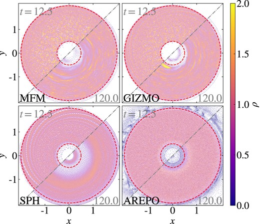
Evolution of the Kepler disc using different hydro-methods. Surface density at two times per method: t = 12.5 (upper left) and t = 120 (lower right). In general, all methods are able to evolve a stable disc. Initial perturbation introduced by the ICs, however, evolve differently for the different methods.
Initially, all methods produce spirals as a result of perturbations in the ICs. While for more traditional SPH with Balsara viscosity switch (Balsara 1998) these lead to a destruction of the disc after only a few orbits, consistent with the results of Beck et al. (2016a), the modern SPH implementation in OpenGadget3 with the improved viscosity scheme of Beck et al. (2016a) drastically increases the stability of the disc. While the inner and outer regions still show some decay, the main part of the disc is stable for the whole evolution considered. For MFM, the disc remains stable for more than 20 orbits. We observe that the inner and outer parts of the disc degrade much less compared to SPH. The initial perturbations are diffused throughout the disc, which shows slightly larger perturbations in the main part compared to the SPH calculation. Both, our implementation and the one in gizmo, show qualitatively similar results. The Arepo run turns out to produce the most stable disc. Only a slight degeneration at the boundaries can be observed. Further studies would be needed to analyse whether this is a numerical effect or due to interaction with the ambient medium not present in the other calculations.
4.3 Tests for fluid mixing instabilities
Mixing occurs in a variety of cosmological situations, most prominently during ram-pressure-stripping. To this end, we analyse the ability of the different codes and methods to evolve such mixing instabilities.
4.3.1 Rayleigh–Taylor instability
One popular fluid-mixing test is the Rayleigh–Taylor instability. It can be used to explore how well the code can describe unstable growing modes. The set-up we use is taken from Hopkins (2015). The calculations are preformed in a two-dimensional periodic box with side-lengths 1, populated with 65 536 particles where the particles at y < 0.1 and y > 0.9 are fixed as boundary conditions. In contrast to the other codes, for Arepo the boundary particles are not fixed but instead a relflective boundary condition is used.
A fluid of high density (ρ = 2) is placed on top of a low-density medium (ρ = 1) in hydrostatic equilibrium. For this test-case, we take γ = 1.4, as for a diatomic gas, such as molecular hydrogen and apply the constant gravitational acceleration
To allow the instability to grow, a small velocity perturbation at the phase boundary is introduced (for more details see Hopkins 2015).
In Fig. 5, we show that all methods are perfectly able to evolve the instability.
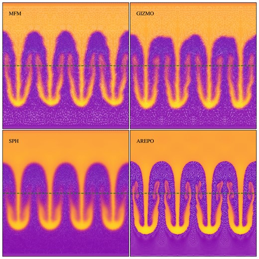
Rayleigh–Taylor instability at time t = 3.6. Comparison between the different hydro-methods. Vertical line marks the initial position of the phase boundary. Differences are mainly the presence or absence of secondary instabilities.
A major difference between the different methods is the presence of asymmetries and secondary instabilities. While these can be seen clearly for MFM, both in OpenGadget3 and gizmo, and are also present in the Arepo calculation where they appear more symmetric, we find that they are absent from the SPH calculation, due to the smoothing over the larger kernel and the effectively lower spatial resolution (e.g. Marin-Gilabert et al. 2022, for a more detailed discussion of the occurance of secondary insatbilties and their physical meaning). The results of Arepo indicate the sharpest boundary and highest density in the tip, followed by MFM. The particles close to the boundary for Arepo show still a clear imprint of the initial grid-like particle distribution. We note that the numerical diffusivity within modern SPH causes the boundary of the instability to have a shallower gradient and smears out initial asymmetries. In addition, the effective spatial resolution is lower by a factor of ≈2 compared to MFM due to the larger neighbour number and thus SPH reaches a much lower density in the tip of the instability.
4.3.2 Kelvin–Helmholtz Instability
Similar to the Rayleigh–Taylor instability, also the Kelvin–Helmholtz instability is a famous example for fluid mixing. Again, we use the set-up provided by Hopkins (2015). Two fluids of densities ρ1 = 1 and ρ2 = 2 in hydrostatic equilibrium are initialized in a 2D periodic box, with initial velocities |${\boldsymbol v}_{1}=0.5\hat{x}$|, |${\boldsymbol v}_{2}=-0.5\hat{x}$| and a small perturbation following McNally, Lyra & Passy (2012). The set-up includes in total 774 144 particles. At time t = 2.5 corresponding to ≈1.2τKH in units of the Kelvin–Helmholtz time-scale |$\tau _\mathrm{KH}=\frac{\lambda }{\Delta v_x}\frac{\rho _1+\rho _2}{\sqrt{\rho _1\rho _2}}$| (compare e.g. Junk et al. 2010), the instability has produced a roll for all methods, as shown in Fig. 6.
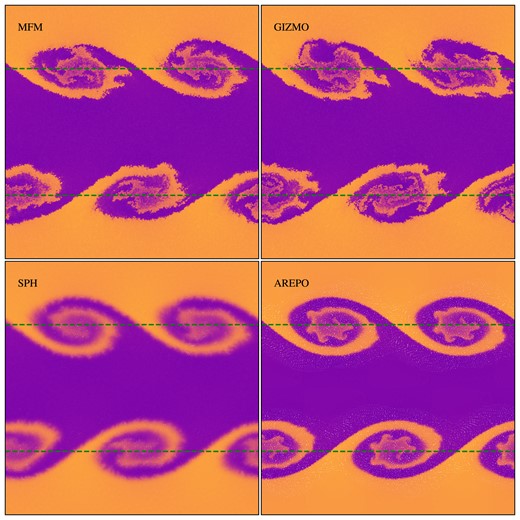
Build-up of a 2D Kelvin–Helmholtz instability at t = 2.5 comparing different methods. Horizontal dashed lines mark the initial position of the phase boundary. All methods produce the roll, but with differences in their inner structure.
Differences are present in the inner structure of the roll. Overall, the qualitative results are very similar to those for the Rayleigh–Taylor instability. SPH is smoothing the roll, showing no secondary instabilities and evolving more smoothly towards later times. Compared to that, MFM in both implementations shows a clear separation between the higher-density roll and the less dense medium, with the presence of secondary instabilities. A more detailed analysis of the Kelvin–Helmholtz instability, also using our new MFM implementation, has been done by Marin-Gilabert et al. (2022). They also show that the secondary instabilities can be avoided by using a higher neighbour number in combination with a higher-order kernel. This will increase the intrinsic viscosity and prevent mixing in form of secondary instabilities. Also, Arepo shows secondary instabilities, present especially inside the roll. When present, these perturbations will finally dominate the evolution over the build-up of the roll for t ≳ 3.
4.3.3 Hydrostatic square
As both aforementioned fluid-mixing tests contain sharp boundaries that deform due to instabilities, the understanding of the evolution of such boundaries evolving without perturbations imprinted in the ICs is important. The Hydrostatic square tests this behaviour, as it is well suited to study the stability of edges related to numerical surface tension. Similar tests have been performed e.g. by Hess & Springel (2010) and Hopkins (2013, 2015).
We set up a two-dimensional box of size L = 1 with periodic boundary conditions. It is filled with 7168 gas particles with equal masses, arranged in two regular grids, one grid for the ambient medium (ρa = 1, Pa = 2.5) and one for the square with side-length L/2 with increased density ρs = 4 in hydrostatic equilibrium (Ps = Pa). In Fig. 7, we compare the resulting density distribution at time t = 10, evolved with the different methods.
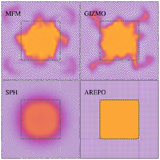
Density of the hydrostatic square evolved until t = 10 using different methods. The initial location of the high density ‘square’ region is overplotted as contour. Only Arepo is able to keep the initial square shape, while other methods lead to deformation of the square.
As the ICs are set in hydrostatic equilibrium, we would expect no changes to occur. This ideal state is only achieved using the moving mesh code Arepo. Theoretically, we would expect the same to be true for MFM, as shown by Hopkins (2015). They use, however, a strongly idealized set-up compared to ours. Especially, they use a regular grid for all particles, and increased particle masses within the square. For our set-up, the gradient estimate at the boundary does not conserve linear gradients. Instead, it is biased by the in-homogeneous particle distribution due to two separate grids, especially in combination with the slope-limiter. A more detailed analysis of the effect of the slope limiter is provided in Section 4.8.1, where we have shown that the amount of surface tension and resulting deformation of the square strongly depends on the slope-limiter. We observe, using both our MFM implementation and gizmo, that for MFM, the edges of the square start to deform, followed by some numerical instability, which leads to a more asymmetric deformation. Increasing the resolution by a factor of 4, as shown in Fig. 8, this instability occurs slower and the square preserves its shape much better.
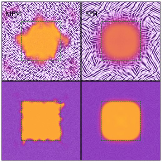
Hydrostatic square at t = 10. Comparison of MFM and SPH at two different resolutions, Top: 7168 particles, Bottom: 114 688 particles (increase in resolution by factor 4. Both, MFM and SPH, show convergence of the shape of the square.
Also using SPH, the square deforms. As expected, it becomes more circular, caused by numerical errors, which behave as surface tension (compare e.g. Price 2008). For traditional SPH, these errors should be low-order. We observe, however, that this effect can be drastically reduced by increasing the resolution, as shown in Fig. 8 indicating that modern SPH implementations, as used in OpenGadget3, reduce low-order errors and improve convergence. Overall, for this specific test surface tension for SPH, but also for MFM can be observed. A moving mesh performs best, preserving the situation perfectly. MFM at later times shows some numerical errors leading to a more asymmetric deformation, which converge away with increasing resolution.
4.3.4 The ‘Blob’ test
A more complex problem is the blob test. It is designed to mimic ram-pressure stripping by an interplay of the evolution of shocks and fluid-mixing instabilities. We use the set-up described by Hopkins (2015) (compare also Agertz et al. 2007). A three-dimensional box with side-length 2000 in x- and y-direction and 6000 in z-direction is populated with 9641 651 particles. A cloud of higher density ρcloud = 10ρwind is placed into a wind tunnel with supersonic flow at |$\mathcal {M}=2.7$| and density ρwind = 2.6 · 10−8. Both phases are set up in pressure equilibrium.
The resulting density in a slice through the cloud at t = τKH and t = 4τKH is shown in Fig. 9.
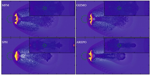
Blob at t = τKH and t = 4τKH as small insertion comparing different hydro-methods. At the earlier time, SPH leads to much less deformation due to less instabilities building up, while MFM in both implementations as well as Arepo agree qualitatively. At late time, MFM and Arepo are fully mixed, while SPH still has some structure remaining.
In front of the cloud, a bow shock forms. At the Kelvin–Helmholtz time-scale τKH = 2, the cloud has developed instabilities. These are much more pronounced for MFM and Arepo, while for SPH, the cloud deforms, without showing instabilities. The precise form of the cloud differs between our MFM implementation, that in gizmo and the moving mesh code Arepo. Nevertheless, the cloud mass, defined by the particles obeying ρ > 0.64ρcloud, i and u < 0.9uamb, i, is very similar for all methods until τKH, shown in Fig. 10. As expected, the MFM calculations line up with the calculations done by Hopkins (2015).
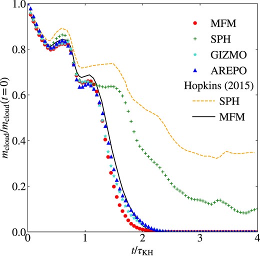
Decay of the cloud fraction surviving for the different methods. In the background, comparison lines of the results by Hopkins (2015) for MFM (black, solid) and (traditional) SPH (orange dashed) are shown. MFM and Arepo agree very well, while SPH shows less mixing.
The periodic bumps are a result of the self-interaction of the shock due to the choice of boundary conditions.
At later times, the evolution strongly deviates. While for MFM as well a moving mesh, secondary instabilities build up and lead to a disruption of the cloud, it is more stable in SPH. Compared to the more traditional SPH results of Hopkins (2015), however, we find the blob to decay stronger, as modern SPH with time-dependent artificial viscosity and conductivity is able to evolve instabilities much better, thus allowing for more mixing.
4.4 Tests for shock-capturing
4.4.1 Sod shock-tubes
Another important capability of the code is to capture strong shocks of (arbitrarily) large Mach number. We begin testing this on a simple Sod shock-tube based on the set-up of Sod (1978). The test is preformed in a three dimensional periodic box of size Lx = 140, Ly = Lz = 1 with two fluids of different density and pressure (ρ1 = 1, P1 = 1; ρ2 = 1/8, P2 = 0.1 for γ = 1.4) that are initialized in a glass-like configuration of in total 216 090 particles. When the two phases start interacting, a shock begins to move to the right. In Fig. 11, we show the resulting structure at t = 2.5 for the MFM calculations at different Mach number and compare them to the analytic solution.
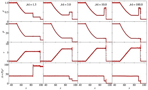
Density, pressure, velocity, and entropy profile of the shock tube at t = 2.5 calculated with our MFM implementation, comparison between different Mach numbers. MFM is able to reproduce the general structure of the shocks. Artefacts of surface tension introduced by the slope-limiter are visible at higher Mach numbers. The scatter is a result of the choice of ICs.
The expected profiles are matched very well, for all the Mach numbers adopted in this work, ranging from a very low |$\mathcal {M}=1.5$| shock to a strong |$\mathcal {M}=100$| shock. This ability is directly connected to the accuracy of the Riemann solver. For higher Mach numbers, increasing peaks in velocity and entropy at the shock front are present as a result of the non-TVD slope-limiting procedure, which has also been reported by Hopkins (2015). We note that this peak and nearby oscillations would be even larger of no limiter was used, and can be avoided even better by using a TVD-limiter, which has more disadvantages in other cases. With increasing Mach number, a sufficiently small time-step becomes more important. The scatter in velocity for the high |$\mathcal {M}=100$| shock, as well as the small offset in the position of the shock front converge away with decreasing time-steps.
The scatter in density present at all Mach numbers is a result of the choice of the ICs, which are set up in a glass-like configuration and designed for a higher neighbour number. It does not converge for low neighbour numbers, as chosen for MFM. The pressure profile shows the typical bump at the rarefaction fan, as well as the pressure blip at the contact discontinuity, shown in more detail in Fig. 12 for the intermediate |$\mathcal {M}=10$| shock. This indicates the presence of surface tension-like error terms, introduced by the slope limiter.
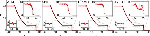
Pressure profile of the |$\mathcal {M}=10$| shock tube at t = 2.5, comparison between different hydro-methods. The different codes show different amount of surface tension and also slight differences in the position of the shock front due to different time-stepping.
As discussed in Section 4.3.3 on the example of the hydrostatic square, these terms are present for SPH and both MFM implementations, but not for Arepo, manifesting also in the presence or absence of the pressure blip for the different methods. The shock front is captured equally well for MFM and SPH, though less smoothed out for MFM due to the lower neighbour number. Arepo poorly captures the behaviour at the shock front. Especially, it has troubles in the mesh reconstruction in this strongly anisotropic region, which leads to a shift in the position of the shockfront and to the oscillatory behaviour in the shocked region. It could be improved using a static mesh, which would remove other advantages of this method, however.
4.4.2 Sedov–Taylor blastwave
This very strong radially symmetric shock has first been introduced by Sedov (1946, 1959). Besides the capability to deal with jumps, Saitoh & Makino (2009) describe how it can be used to analyse the time-step limiter and shows the need for the limiting to be non-local, as provided by the wakeup scheme. The test has become a popular benchmark for Supernova blast wave evolution in recent years (e.g. Kim & Ostriker 2015; Steinwandel et al. 2020).
As ICs, we set up a regular grid with 643 particles and density ρ = 1. While almost all particles exhibit a vanishing pressure Pa = 10−6, energy of U = 10 is distributed equally into the eight central particles. A shock with very high |$\mathcal {M}_i\gtrsim 2\cdot 10^{4}$| arises, and quickly moves outwards.The radial density distribution is shown in Fig. 13.

All methods are able to capture the shock, though slightly smoothing it, thus underestimating the height of the density peak. SPH shows the strongest smoothing, followed by the two MFM implementations. Arepo is able to reproduce the height of the peak best.
The position of the peak is similar for all methods, with minor differences. While Arepo and gizmo’s MFM implementation predict the peak position correctly, MFM and SPH in OpenGadget3 lag slightly behind, which results in a more accurate position of the low-density side of the shock. This position strongly depends on the precise time-step settings, indicating differences in the time-stepping between the codes.
4.5 Including self-gravity
In cosmological contexts, not only hydrodynamical forces, but also gravitational accelerations are of great importance. Gravity dominates the evolution on large scales due to its long-range character. It can lead to collapse of clouds, e.g. in the ISM for star formation, or balance thermal pressure and lead to hydrostatic equilibrium, such as in the global structure of galaxies or galaxy clusters. Thus, we analyse the interplay between hydrodynamical forces and gravity in the following.
4.5.1 Gravitational freefall
As a first test including self-gravity, we simulate a collapsing sphere. The ICs are set up on a regular grid of 203 particles and cut out a sphere of radius 1, which has a total mass of Msphere = 1 and a negligible pressure of P = 10−6. For the Arepo run, we fill the region not occupied by the sphere with low mass, low energy particles at resolution of only 8 particles per unit length, arranged in a regular grid, in order to improve the mesh reconstruction at the boundary. We follow the evolution of the half-mass radius, to not be influenced by boundary effects as for the full radius, shown in Fig. 14.
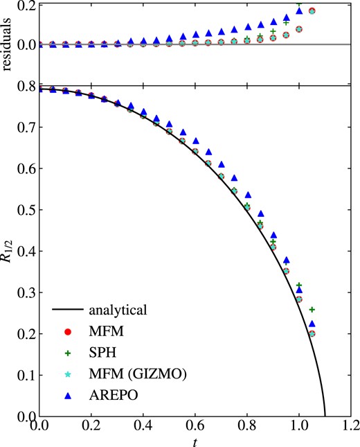
Evolution of the half-mass radius for the gravitational freefall test. All methods agree at early time, but deviate from the expected solution at later times when hydrodynamical contributions become more important.
Comparing to the analytic solution for a purely gravitational freefall
all methods agree at early times. At late times, pressure and thus effects of the hydro-scheme become more relevant, and deviations are visible. For all methods, additional pressure contributions lead to an increase in radius as it would be expected. As the initial pressure is small, only a small deviation is expected. MFM lies closest to the ideal solution with both implementations being indistinguishable. The moving mesh code Arepo overestimates the radius already at early times, which can be explained by poor treatment of the non-periodic boundary conditions. While gravity is calculated in a non-periodic way, the mesh construction for the hydro-calculation requires the box to be treated periodically, which is not the case for all other methods. Including the low-mass cells at the boundary already decreased the error by a factor of 2 and it could be further decreased by enlarging the box. SPH lies in between the other methods except at very late times, when the deviation strongly increases due to oversmoothing.
4.5.2 Hydrostatic sphere
In cosmological contexts, e.g. for the ICM, the ability of the code to preserve hydrostatic equilibrium against gravity is of great importance. To test this, we calculate a hydrostatic sphere as a second test including self-gravity. It is also the first test including dark matter as second, only gravitationally interacting particle type. The ICs have been created following Viola et al. (2008). 88 088 DM particles are set up following an NFW profile (Navarro, Frenk & White 1997), populated with 95 156 gas particles in hydrostatic equilibrium. The corresponding density and internal energy profiles at different times are shown in Fig. 15.
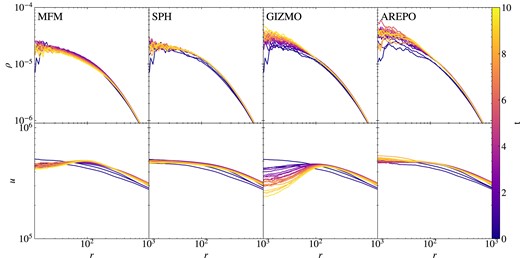
Evolution of gas density (top) and internal energy radial profiles (bottom) for the hydrostatic sphere for approximately 10 dynamical times until t = 10, coloured by the time. Calculated using different hydro-methods. MFM shows a slightly larger numerical diffusivity, but overall still preserves the density profile.
After a short relaxation period, happening on a time-scale approximately corresponding to the dynamical time tfreefall ≈ 1 at r = 102, we expect the gas to keep hydrostatic equilibrium. SPH as well as our MFM implementation show the lowest deformation in density. MFM in gizmo, as well as Arepo show a slightly stronger increase in density, especially in the central region. While the density is only an indirect tracer of (numerical) diffusivity, the internal energy profile is more directly affected by it. Thus, it can give even more insight into the convergence over time.
For SPH, we observe a stable situation to be reached within one freefall time, and only minor changes to the initial profile. The same is true for MFM in OpenGadget3, where changes in internal energy are only marginally larger compared to SPH. For Arepo, changes compared to the initial profile are similar to the MFM result, as the initial conditions were designed assuming SPH. After a similar time-scale for this relaxation, also for this method a stable situation is reached. For MFM in gizmo, in contrast, an impact of the numerical diffusivity can be observed. Resulting mixing in the central region leads to a decrease in internal energy, leading to the observed increase in central density. Differences between the MFM implementations are results of the different Riemann solver in combination with fine differences of the implementation. Also in previous implementations of ours, we observed a similar change as for gizmo. Over very long time-scales, the sphere would tend to become isothermal for MFM. Despite these findings, the effect on the density profile is quite small for all methods over the time-scale considered.
4.5.3 Zeldovich pancake
The Zeldovich pancake is the first problem to test our implementation of comoving integration. In addition, it is well suited to show effects of very high |$\mathcal {M}$| flows, shocks, highly anisotropic particle arrangements, and also very low-internal energies. It has been introduced by Zel’dovich (1970). We start our calculation at zi = 100, setting up a single Fourier mode density perturbation. During the linear growth until the caustic formation at zc = 1, the evolution can be described by
starting from the unperturbed position xi. ρc is the critical density, H0 = h0 · 100 km s−1 Mpc−1 the Hubble parameter (today) with h0 = 1, and Ti = 100 K the initial temperature, such that pressure forces are negligible. The wavenumber k = 2π/(64 h−1 Mpc) corresponds to the first-order soundwave. We use the ICs provided by Hopkins (2015), with a resolution of 323 particles. After the linear growth, an accretion shock forms close to the centre. As the scale factor increases, the background density decreases strongly and the background temperature decreases adiabatically. This causes a huge temperature contrast of ≈10 orders of magnitude between the shocked region and the background. Due to the very low-internal energy compared to other energy contributions U ≲ 10−3Ekin and U ≲ 10−2Epot in physical units, the evolution can be strongly dominated by numerical errors. Thus, the implementation of the energy-entropy switch described in Section 3.3 is important. The precise limits, when the switch is supposed to be active, are related to the numerical accuracy and details of the implementation such as the precision of the Riemann solver. The effect of the limits chosen on the evolution of the Zeldovich pancake is described further in Section 4.8.2.
The resulting structure at z = 0 is shown in Fig. 16. Again, we compare the performance of the different hydro-methods. The energy-entropy switch is included for MFM in OpenGadget3 if U < 0.01Epot, corresponding also to the value implemented in gizmo. For Arepo, we had to use additional mesh regularization to avoid too irregular cell shapes in the highly unisotropically compressed shock region and allow the code to run until the end. All methods agree with the peculiar velocity profile with only slight differences. Compared to Hopkins (2015), we find that all methods seem to have a too low viscosity and show particle over or undershooting compared to the predicted velocity profile, as a result of a punch-through of some particles in the high |$\mathcal {M}$| shock. One difference between the methods is the height of the density peak. This is the lowest for sph, which can be explained by the larger kernel for SPH, leading to stronger smoothing, compared to MFM. Thus, MFM in OpenGadget3 is able to resolve the central region better and has a slightly higher peak. The Arepo run shows an even higher peak, contrarily to what Hopkins (2015) found. Compared to the expected profile, all these methods oversmooth the central region. The gizmo code captures the density profile best, reaching the highest central peak. Most difficult for all methods is to capture the temperature structure with its very strong contrasts. Both MFM implementations work very well, as the energy-entropy switch suppresses any numerical noise in the low-energy background and allows a clear jump between shocked and unshocked region. Slight differences in the implementation of the energy-entropy switch between OpenGadget3 and gizmo, as well as a lower temperature in the central region in general result in more particles in the centre, being treated with the switch for gizmo, resulting in a larger number of cold particles. This difference can also explain the different height of the density peak. As we will show in Section 4.8.2, a less aggressive switch will result in a higher density peak. As no analytical solution exists for this test, it is unclear if this behaviour is wanted. The jump for SPH is more strongly smoothed in comparison to the other methods. In addition, amplified initial (numerical) noise causes a large scatter of several orders of magnitude in the very cold background. For Arepo, we find that this behavior is much more drastic, and the background is dominated entirely by numerical noise. To properly resolve it, some energy-entropy switch would be required also in Arepo, which does not seem to be implemented in the public version.

Zeldovich pancake at z = 0 for different hydro-methods. As a comparison, a high resolution 1D simulation of Hopkins (2015) is shown. While velocity and density profiles agree between the methods, strong deviations can be seen for the temperature profile. MFM performs best due to the energy-entropy switch employed.
4.5.4 Nifty cluster
Finally, we apply our newly implemented method on more complex, cosmological cases. As an example, we resimulate a cluster from the MUSIC-2 sample (Prada et al. 2012; Sembolini et al. 2013, 2014; Biffi et al. 2014), analysed in detail with different codes by a collaboration formed during a nifty workshop (Sembolini et al. 2016), thus called nifty cluster in the following. The cluster has a mass M200c = 1015 M⊙ with resolution mDM = 9.01 · 108 h−1 M⊙ for dark matter and mgas = 1.9 · 108 h−1 M⊙ for gas particles. The background cosmology has parameters |$\Omega _{\text{M}}=0.27,\Omega _{\text{b}}=0.0469,\Omega _\Lambda =0.73,\sigma _8=0.82,n=0.95,h=0.7$| (Komatsu et al. 2011). The projected surface density at z = 0 is shown in Fig. 17, where the cluster center and virial radius are obtained using subfind (Springel et al. 2001; Dolag et al. 2009).
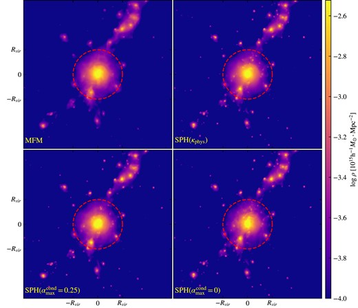
Projected surface density of the nifty cluster at z = 0, comparison between MFM and SPH with usual amount (|$\alpha _{\max }^{\text{cond}}=0.25$|), physical (κphys), corresponding to an intermediate amount, and without artificial conductivity |$\alpha _{\max }^{\text{cond}}=0$|. The overall structure is very similar. Small sub-structures, however, appear less compact for MFM.
We compare MFM to SPH with a different amount of artificial conductivity, ranging from the usually used amount αmax = 0.25, αmin = 0 (notation following Price 2008) over a run with physical conductivity at 1/20th of the Spitzer value (Dolag et al. 2004), effectively corresponding to an intermediate amount, to more traditional SPH without artificial conductivity. The usual amount is chosen to mimic the behaviour of Godunov methods such as MFM, which have intrinsic numerical diffusivity due to the Riemann solver and thus allow for more mixing. The structure looks very similar between MFM and SPH with standard settings. This will change, however, for different values for artificial conductivity. For reduced artificial conductivity, structures are slightly less ‘smeared out’, while the global structure does not change.
A more quantitative analysis can be done using gas radial density, temperature and entropy profiles shown in Fig. 18.
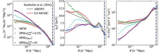
Gas density (left), temperature (middle), and entropy (right) radial profiles of the nifty cluster at z = 0, comparison between different hydro-methods, including our MFM implementation (red plus), SPH in OpenGadget with usual (green), physical, corresponding to an intermediate value, (turquoise), and without artificial conductivity (blue). As a comparison, the Arepo (black dashed) and G3-MUSIC (traditional) SPH line (red solid) from Sembolini et al. (2016) are shown. The vertical line marks R200. Our modern SPH run with sufficiently high artificial conductivity, as well as Arepo and MFM produce higher entropy cores with lower less peaked density, while the central entropy is much lower for SPH with lower artificial conductivity.
As a comparison, we provide lines from the nifty paper, obtained using Arepo and Gadget3-MUSIC as an example of a more traditional SPH code, which mark the range of solutions obtained. SPH can span the whole range of possible solutions provided by Sembolini et al. (2016). By construction traditional SPH without artificial conductivity has no mixing and thus forms low-entropy cores. Subgrid mixing due to the Riemann solver for MFM and Arepo leads to mixing into the core, increasing the entropy compared traditional SPH. Thus, the central density is reduced. By including artificial conductivity in SPH, it can reach the same profile as MFM, and also lie in between for effectively intermediate values by using physical conductivity.
4.6 Decaying sub-sonic turbulence
In many astrophysical systems, ranging from the atmosphere over the ISM up to galaxy clusters, turbulence plays a crucial role. In the ICM, we expect sub-sonic turbulence with a turbulent energy fraction of X ≈ 0.1 to be excited, for instance after a merger (compare e.g. Schuecker et al. 2004; Subramanian et al. 2006). The different hydro-schemes have problems to capture its full behaviour. It has been shown that traditional SPH is not well suited to calculate sub-sonic turbulence (Bauer & Springel 2012), but can be improved using modern SPH with more ideal settings for artificial diffusion terms (Price 2012). While grid based methods produce better results, difficulties still remain for the evolution of turbulence within galaxy clusters.
To test and compare the performance of our MFM implementation, we set up a 300 kpc cubic box with varying number of particles, and seed the largest ≈70 modes, similar to Bauer & Springel (2012). Due to the low-initial density of ρ ≈ 1.5 · 10−6, gravitational acceleration can be neglected. The initial turbulent energy fraction is varied between Xi = Eturb, i/Etherm, i = 0.3, corresponding to a Mach number |$\mathcal {M}_i\approx 0.7$| and Xi = 0.00001 corresponding to |$\mathcal {M}_i\approx 0.004$|. In addition, the resolution is varied, ranging from 643 up to 2563 particles. We evolve the turbulence for 1.5 sound-crossing-times. The turbulent kinetic energy cascades down to smaller scales, forming a turbulent power spectrum. In order to analyse the velocity power spectrum, the data are binned to a grid using the code sph2grid.5 From that, a power spectrum is calculated. We use a D20 sampling, to conserve energy (Cui et al. 2008). Theoretically, a Kolmogorov slope E(k) ∼ k−5/3 would be expected (Kolmogorov 1941). In Fig. 19, we compare the power spectra of the different methods, normalized by the expected slope. The wavenumber kbox corresponds to a wavelength of the box size. Energy is seeded between kSEED, max and kSEED, min. An estimate for the resolution limit is provided by |$k_{\text{SML}}^{128}$|, corresponding to the mean smoothing length for a Wendland C6 kernel at resolution 1283 in plots where an SPH run is included, otherwise to the mean smoothing length for a cubic spline kernel at resolution 1283, and |$k_{\text{Nyquist}}^{128}$| denoting wavenumber of the initial grid-spacing and thus the smallest length to be possibly resolved.
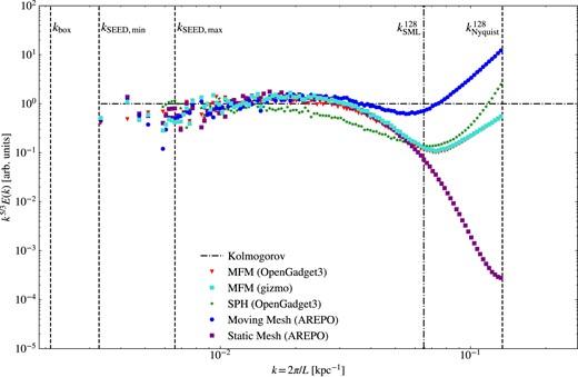
Normalized turbulent velocity power spectrum for different methods at Xi = 0.3 and resolution 1283. All methods agree at large scales, but show a lack in energy at intermediate to small scales compared to the expected Kolmogorov-slope P ∼ k−5/3. Overall, all methods work very well reproducing the expected spectrum.
In contrast to many previous findings (compare e.g. Padoan et al. 2007; Bauer & Springel 2012; Hopkins 2015), all methods are able to reproduce the expected Kolmogorov slope very well for such a mildly sub-sonic turbulence. SPH shows the strongest deviation, occurring already at intermediate scales, while for MFM in both implementations and also arepo with moving and stationary mesh, differences are present only at very small scales, approaching the resolution limit.
In addition, the MFM result converges quickly with resolution, shown in Fig. 20. As the dip moves towards smaller scales, the overall spectrum becomes even closer to the Kolmogorov one over a wider range of scales. At the highest resolution considered, it almost perfectly resembles the expected Kolmogorov slope over almost on order of magnitude of scales.
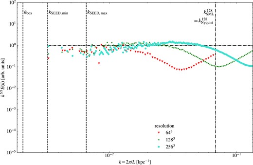
Normalized turbulent velocity power spectrum for MFM with different resolutions at Xi = 0.3. MFM converges fast with resolution towards the expected Kolmogorov-slope P ∼ k−5/3.
For even lower initial turbulent energy fractions, corresponding to even lower Mach numbers, more differences between the methods become visible. In Fig. 21, we show the resulting spectrum for an initial turbulent energy fraction of 0.01, corresponding to |$\mathcal {M}_i\approx 0.1$|. While all methods agree at large scales, where the energy was seeded, they show huge discrepancies at intermediate to small scales. Arepo shows deviations at the smallest scales compared to the other methods, underestimating the energy present at scales close to the resolution limit. SPH starts deviating at slightly larger scales, with a less deep dip in the power spectrum. For MFM, the power spectrum shows a dip in energy at similar scales as the moving mesh code Arepo, but with a much shallower depth than in all other cases, thus being closer to the expected slope. Differences between the two MFM implementations can be attributed to different Riemann solvers used. Overall, advantages of MFM become clear for such very subsonic turbulence.
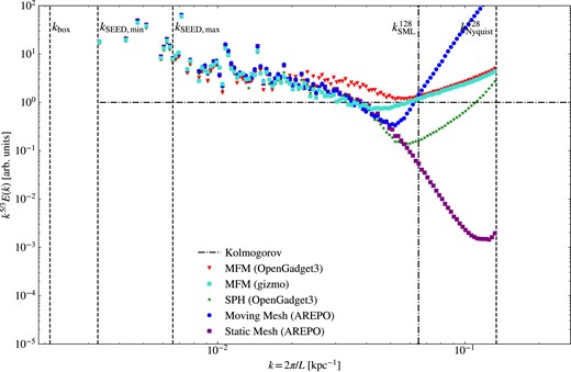
Normalized turbulent velocity power spectrum for different methods at Xi = 0.01 and resolution 1283. At such low initial turbulent energy fraction, differences between the methods become more visible, where MFM works best overall reproducing the expected spectrum.
While the power spectrum builds up, energy is not only transported to smaller scales, but also partly converted into internal energy. We plot this decay of kinetic, turbulent energy, here labelled with E, in Fig. 22, comparing the different hydro-methods. In order to better compare the slopes independent of initial turbulent energy fraction, we fit an exponential decay for each run and normalize by |$E^{\text{fit}}_i=E^{\text{fit}}(t=0)$|. While in a physical situation the decay would depend on gas microphysics such as its viscosity, here we can use it to get an insight into the code behaviour. The decay is mainly determined by numerical dissipation.
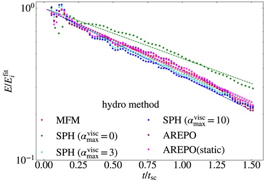
Decay time of turbulent energy for different methods at Xi = 0.3. For SPH, the viscosity is varied between |$\alpha _{\max }^{\text{visc}}=10$| and |$\alpha _{\max }^{\text{visc}}=0$|, where |$\alpha _{\max }^{\text{visc}}=3$| is the value typically used (notation following Beck et al. 2016a). Arepo has the highest decay time corresponding to the lowest numerical dissipation, while MFM and SPH at typical value of viscosity are on a similar order with a decay time of a few dynamical time-scales.
In all cases, the energy shows a periodic variation, caused by the ‘ringing’ of the initially seeded modes. The decay for SPH depends mildly on the artificial viscosity especially visible for the run excluding it. The power spectrum, in contrast, is only weakly influenced by the amount of artificial viscosity. In practical applications, it is tuned to a value of |$\alpha _{\text{max}}^{\text{visc}}=3$|, which leads to a similar decay rate as the other methods. The exponential decay time tdec roughly corresponds to the sound crossing time tsc = Lbox/cs.
A comparison for the decay at different initial turbulent energy fractions, corresponding to variations in the Mach number, is shown in Fig. 23 for MFM and SPH.The variation between 0.3 and 0.000 01 for the initial turbulent energy fraction corresponds to a range of Mach numbers from 0.7 down to below 0.004. For SPH, the decay is decreasing with initial turbulent energy fraction down to Xi = 0.01 (|$\mathcal {M}\approx 0.1$|), and stays independent of the Mach number afterwards, as one would expect, so it is for arepo. For MFM, the same initial trend can be observed. For very low initial turbulent energy fraction Xi < 0.0001 (|$\mathcal {M}\lesssim 0.01$|), however, an unphysical increase of turbulent energy occurs. At the same point also the density pdf deviates from the Gaussian shape together with the velocity power spectrum becoming strongly non-Kolmogorov, indicating the evolution is dominated by numerical artefacts for such low Mach numbers. Specifically, while we find that for this test total energy is conserved the internal energy only accounts for a small fraction, such that even evolving internal energy instead of total energy will be dominated by numerical errors. Applying an energy-entropy switch could in principle alleviate this problem. On the other hand, it would be unclear if this would remove other advantages for MFM in this test problem.
4.7 Runtime analysis
The precise difference in wallclock runtime between MFM and SPH depends on the problem that is considered, as this can include different additional physics and might trigger different time-step limiters. Therefore, we provide an overview of all runtimes for the tests that we have run, including the MPI and OpenMP configuration in Table 1.
Comparison of the runtime between MFM and SPH in OpenGadget3. Different test are run with different MPI and OpenMPI configurations and also on different machines. In general, we observe an increase in runtime between MFM and SPH, varying between a factor of ≈2 for pure hydrodynamical tests to only a factor of 1.1 for the nifty cluster.
| test | MPI | OpenMP | runtime [s] | time per time-step [s] | #steps | |||
|---|---|---|---|---|---|---|---|---|
| MFM | SPH | MFM | SPH | MFM | SPH | |||
| soundwave (res 128) | 4 | 14 | 4.3 · 104 | 3.2 · 104 | 5.3 · 100 | 7.9 · 100 | 8.1 · 103 | 4.1 · 103 |
| kepler disc | 4 | 14 | 4.1 · 105 | 5.4 · 105 | 8.1 · 100 | 8.0 · 100 | 5.1 · 104 | 6.8 · 104 |
| Rayleigh–Taylor instability | 4 | 14 | 8.4 · 103 | 3.4 · 103 | 2.6 · 10−1 | 1.1 · 10−1 | 3.2 · 104 | 3.0 · 104 |
| Kelvin–Helmholtz instability | 8 | 12 | 6.7 · 105 | 2.9 · 105 | 1.0 · 101 | 8.8 · 100 | 6.5 · 104 | 3.2 · 104 |
| Hydrostatic square | 4 | 14 | 1.9 · 102 | 7.1 · 101 | 2.3 · 10−2 | 1.6 · 10−2 | 8.2 · 103 | 4.2 · 103 |
| blob test | 8 | 12 | 2.5 · 106 | 1.5 · 106 | 1.3 · 102 | 1.4 · 102 | 1.9 · 104 | 1.1 · 104 |
| shock tube (|$\mathcal {M}=10$|) | 4 | 14 | 8.9 · 103 | 1.7 · 103 | 1.1 · 100 | 7.7 · 10−1 | 8.2 · 103 | 2.1 · 103 |
| Sedov blast | 4 | 14 | 1.1 · 102 | 1.9 · 102 | 2.1 · 10−1 | 2.5 · 10−1 | 5.3 · 102 | 7.8 · 102 |
| gravitational freefall | 4 | 14 | 1.3 · 101 | 1.7 · 101 | 5.1 · 10−2 | 6.6 · 10−2 | 2.6 · 102 | 2.7 · 102 |
| hydrostatic sphere | 4 | 14 | 1.3 · 104 | 1.9 · 104 | 8.2 · 10−1 | 1.2 · 100 | 1.6 · 104 | 1.6 · 104 |
| zeldovich pancake | 4 | 14 | 1.6 · 103 | 2.5 · 103 | 1.1 · 100 | 1.6 · 100 | 1.5 · 103 | 1.5 · 103 |
| nifty cluster | 16 | 28 | 2.6 · 104 | 2.3 · 104 | 1.7 · 100 | 1.4 · 100 | 1.5 · 104 | 1.6 · 104 |
| turbulence (resolution 128) | 8 | 12 | 1.2 · 105 | 4.9 · 104 | 2.4 · 101 | 1.6 · 101 | 5.1 · 103 | 3.1 · 103 |
Overall, the computational costs for running MFM are comparable to those of SPH. For pure hydrodynamical problems the number of time-steps required increases together with the effective spatial resolution by a factor of ≲2. It can be even larger for strong shocks due to the more strict time-step limiting at higher spatial resolution. The CPU-time required per time-step is very similar between the methods. While the Riemann solver is more expensive than the calculation of hydrodynamical accelerations for SPH, and also additional neighbour loops are required for MFM, the lower neighbour number leads to a decrease in computational costs. Depending on the problem, the time required per time-step can be smaller or larger than the time required for the SPH comparison run. In combination, these effects on average lead to slightly larger total runtimes by a factor of ≈2 for MFM.
If gravity is included, the simulation time-step is dominated by the gravitational interactions in many cases, such that a similar number of time-steps is required, independent of the hydro-method. Also, the time spent per time-step becomes even more similar, as the computation of gravitational interaction, which is calculated in the same way for MFM and SPH, is contributing as well.
If even more modules are activated, such as subfind, as it is done for the nifty cluster, the runtime is mainly determined by the precise evolution. For the nifty cluster, we found a slight increase in runtime for MFM, but it can be different for other objects simulated. If even more physics was turned on, we expect differences to become even smaller.
Memory requirements are mainly defined by the size of the particle structures. As MFM holds more variables in the gas particle structure, it is larger by a factor of ≈2 compared to SPH. It could be improved by making more efficient use of existing SPH data and avoiding duplication which are currently still present. The total memory requirement is thus larger by a factor of ≈1.3–2 for pure hydro problems and ≈1.5 for the nifty cluster. Including more physics, the difference would become negligible.
4.8 Effects of numerical parameters
The performance of the numerical methods strongly depends on the precise parameters used. Effects of neighbour number and kernel have already been analysed in detail by various authors (compare e.g. Dehnen & Aly 2012; Tricco & Price 2013; Hu et al. 2014) for SPH. To this end, we focus on two other parameters that play a major role for MFM, namely the slope-limiting scheme and the energy-entropy switch.
4.8.1 Slope-limiter
The different slope-limiting procedures, which are implemented in our code, differ not only in how aggressively they limit the slope, but also in how much numerical diffusivity they introduce. In general, different limiters are shown to produce different results for specific test cases (compare e.g. Barth & Jespersen 1989; Balsara 2004; May & Berger 2013; Hubber et al. 2018; Alonso Asensio et al. 2023).
In the following, we compare the three cases of the limiter from gizmo as described by equation (A6) in combination with their pairwise limiter (equation A10 and A11), that we usually use, the arepo (equation A5) and, the TVD limiter (equation A3). The gizmo and TVD limiters are the most extreme cases of the limiters implemented, with lowest and highest numerical diffusivity, respectively. The Arepo limiter lies in between. We analyse the effect on the hydrostatic square (compare also Section 4.3.3) and the Rayleigh–Taylor instability (Section 4.3.1). The results are shown in Fig. 24.
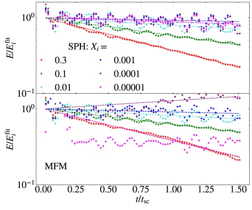
As Fig. 22, but for varying initial turbulent energy fractions Xi, corresponding to variations in the turbulent Mach number. The decay is consistent for all Xi for SPH, and down to Xi = 0.003 for MFM, when numerical artefacts lead to an unphysical increase in energy.
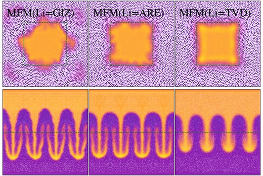
Hydrostatic square (top) and Rayleigh–Taylor instability (bottom), developed using different slope limiters, the gizmo limiter we usually use (left), compared the same test, but evolved using the Arepo limiter (middle) and TVD limiter (right). Depending on the test, different slope-limiters could be preferred.
While for the Rayleigh–Taylor instability the much less diffusive gizmo limiter performs best, evolving a much finer structure, this causes the strongest deformation of the hydrostatic square. The Arepo limiter is slightly more diffusive, leading to less strong secondary instabilities for the Rayleigh–Taylor instability and slightly less deformation of the square, especially at the edges. The TVD limiter has an even higher numerical diffusivity, thus strongly smooths the Rayleigh–Taylor instability, not only preventing secondary instabilities to form, but also noticeably reducing the overall growth of the instability. The hydrostatic square, however, is preserved best, due to lower surface-tension like errors, which also manifest in the presence of absence of the pressure-blib for shocks.
Combining the results, we show that it is not always clear which slope-limiting procedure would be the overall preferred choice. As, in most cases, the gizmo limiter performs best, we chose this as our reference method.
4.8.2 Energy-entropy switch
To avoid numerical errors to dominate the evolution of the internal energy, an energy-entropy switch as described in Section 3.3 has to be used in specific problems such as the Zeldovich pancake. Especially, the numerical noise should be suppressed in the very cold, unshocked region, while the shock should not be influenced at all.
The resulting structure at z = 0, comparing different possibilities for the switch based on potential and kinetic energy estimates (compare also equation 46), is shown in Fig. 25.
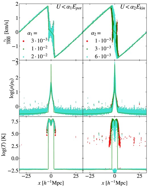
Effect of the choice of the energy-entropy switch on the Zeldovich pancake. Comparison between the switch based on kinetic and potential energy, each with three different α-values. The switch based on potential energy is much more stable.
We increase the tuned values (α1 = 10−2 for the potential energy and α2 = 3 · 10−3 for kinetic energy) by a factor of 2 and decrease them by a factor of ≈3.
A more strict switch (larger α) causes less particles to be treated with the adiabatic approximation. For the kinetic energy switch, this difference causes strong variations in the temperature profiles. While for α2 = 1 · 10−3 more extended wings form and some scatter in the low-temperature background close to the peak appears, the increased value of 6 · 10−3 treats even particles inside the peaked region with the adiabatic approximation and causes too low temperatures. A very fine-tuned choice of α2 is necessary to accurately capture all particles, both the shocked ones and the low-temperature ones.
Compared to that, a variation of α1 within the switch based on potential energy influences the temperature profile only weakly. Thus, it seems to be much more stable and should be the preferred option. We thus used α1 = 10−2 and α2 = 0 for the calculations in Section 4.5.3.
5 DISCUSSION AND CONCLUSIONS
We presented a new MFM implementation into OpenGadget3 as an alternative hydro-solver to the currently used modern SPH. We verified its capabilities, both in idealized and more complex cosmological test cases. Tests range from smooth simple situations, mixing instabilities, shocks, tests including self-gravity, to the nifty cluster as cosmological example and decaying sub-sonic turbulence. A comparison has been preformed between MFM and SPH in OpenGadget3, the MFM implementation in gizmo and the moving mesh code Arepo. In addition, two parameters have been analysed in more detail.
Overall, we find very good agreement between the MFM implementation in OpenGadget3 and that in gizmo. Minor differences are found in the precise appearance, while global properties are indistinguishable in most test cases. Even without further tuning, MFM reproduces the expected behaviour in all test cases considered. The soundwave test is well suited for a convergence analysis, as an analytical solution exists. MFM shows a very good convergence behaviour between first and second order for dispersion errors. Diffusion errors as well as the scatter converge second order. While the convergence is better than for SPH and a moving mesh, these methods show lower errors at low resolution, especially for the dispersion error.
An important advantage of MFM over SPH is the capability to accurately evolve mixing instabilities without additional artificial viscosity or conductivity as for SPH. In addition, a lower neighbour number compared to SPH is sufficient. MFM as well as a moving mesh even show secondary instabilities to occur. The blob test as combination between mixing and shocks emphasizes the ability of MFM to allow for more mixing. The decay rate of the cloud is similar to that of a moving mesh simulation and larger than for SPH. Compared to the more traditional SPH implementation shown by Hopkins (2015), the modern SPH implementation OpenGadget3 allows for more mixing and leads to a faster decay of the cloud. As this test is designed to mimic ram-pressure stripping, we expect this effect to be modelled more accurately using MFM compared to SPH. This should also lead to an overall more accurate evolution of galaxies in the environment of galaxy clusters. To fully understand and follow the evolution of such gas blob in cosmological contexts, more physics such as cooling, and depending on the context, star formation, is necessary. Gronke & Oh (2018, 2020, 2023) have analysed this test in detail with such additional physics and found a great importance of the cooling.
In addition, MFM can model shocks for a wide range of Mach numbers. For the shock tube tests, MFM performs especially well for lower Mach numbers, while effects of surface tension due to the choice of the slope-limiter are visible at higher Mach numbers. Nevertheless, it is still able to capture the main features of the shock including the position of the shock front, the contact discontinuity, and the rarefaction fan. Different methods lead to differences in the smoothing of the shock front. The lower neighbour number in MFM compared to SPH increases the effective spatial resolution by a factor of ≈2. For Arepo, the shock front is dominated by numerical artefacts due to difficulties in the mesh reconstruction in such highly anisotropic region.
The Sedov blast works well for all methods, verifying the capability of the wakeup scheme as non-local time-step criterion. Main differences are the smoothing and resulting lower amplitude of the density peak, revealing an even smaller smoothing for the moving mesh compared to MFM. The narrower shock front will help e.g. for shock detection in cosmological simulations (compare e.g. Pfrommer et al. 2006; Beck, Dolag & Donnert 2016b).
In general, MFM is able to preserve hydrostatic equilibrium accurately, as well as preserving stable orbits. The better stability of the Kepler disc compared to SPH will improve results for simulations of e.g. isolated galaxies. For this case, a moving mesh leads to even better results, but requires additional boundary particles.
The hydrostatic sphere test showed that our MFM implementation coupled to gravity leads to stable hydrodynamical equilibrium, as for SPH and a moving mesh. Depending on the details of the implementation, however, numerical diffusivity can be introduced. Thus, one could expect isolated galaxies or also the core of galaxy clusters to be more compact and cooler in the centre. The time-scales, on which these changes would happen, are, however, very long.
Also, for the nifty galaxy cluster we saw that there is no difference between MFM, Arepo, and modern SPH in the global structure. Numerical diffusivity introduced by the Riemann solver allows mixing of entropy into the core, thus decreasing the central density compared to traditional SPH, which suppresses any mixing. Modern SPH mimics the same effect by applying artificial conductivity, while a variation of the precise amount introduced can lead to significant changes in the structure. As observed galaxy clusters show a wide range of central entropy profiles (Cavagnolo et al. 2009), both results are consistent with observations. Especially, we expect a more complex interplay with cooling, as well as stellar and AGN feedback to influence the entropy evolution of the core (compare e.g. Pearce et al. 2000; Borgani et al. 2005; Rasia et al. 2015). These effects lead to the whole range of possible central profiles, dominating over effects of the hydro-solver. Thus, further studies including such processes would be necessary.
In the intracluster medium, we expect turbulence at low-Mach number to be seeded e.g. by mergers at large scales. It will then decay and build up a turbulent power spectrum. Such decaying, sub-sonic turbulence is a very challenging problem for many hydro-methods. MFM is able to recover the turbulent power spectrum best compared to SPH and a moving and stationary mesh, best visible at very low initial turbulent energy fractions. Only a small lack of energy at intermediate to small scales close to the resolution limit – similar to where this occurs also for Arepo – is present. This ‘dip’ in energy moves to smaller scales for higher resolution, overall leading to fast convergence towards the expected Kolmogorov spectrum.
The decay rate of turbulent energy due to numerical dissipation is on the same order as for modern SPH, and decreases towards higher resolution. The results are consistent down to very small initial turbulent energy fractions Xi = 0.0001, corresponding to small Mach numbers |$\mathcal {M}=0.01$|. For smaller Xi < 0.0001, numerical effects dominate and lead to unphysical increase in turbulent energy. Overall, the results are very promising for the accurate evolution of turbulence also within galaxy clusters.
An energy-entropy switch is of great importance to accurately evolve the temperature profile for the Zeldovich pancake. When it is included, MFM yields the best results, having a clear jump in the temperature. Comparing different possible values for such a switch, we found that careful tuning is required. In general, the switch based on potential energy produces more stable results.
Arepo misses the implementation of such a switch in the public version, such that the low-temperature region is entirely dominated by numerical noise. SPH also shows noise in the low-temperature region, originating from the amplification of noise present in the ICs, and also much broader wings around the peak. All methods show some punch-through in the temperature profile, indicating a too low viscosity.
In addition to comparing different methods, we used two tests to analyse the impact of the slope-limiter. Depending on the problem, different slope-limiters can be preferred. While the gizmo limiter performs best in most test cases, having a much lower numerical diffusivity, specific cases such as the hydrostatic square and also strong shocks work better using a more diffusive TVD-limiter. The Arepo limiter has an intermediate diffusivity and lies in between the two other results.
Overall, our implementation of MFM produces accurate results for the cases considered. It avoids some of the disadvantages of SPH, while requiring a similar computational cost per time-step. The total number of time-steps and thus the total runtime increases as a result of the smaller smoothing length and effectively higher spatial resolution. A faster, approximate Riemann solver can further decrease the computational costs in some cases, but has the drawback of introducing more numerical diffusivity, as discussed in Appendix B. Compared to MFM, a moving mesh requires a very expensive tessellation to be performed, such that the required computational costs for many tests are drastically increased.
Overall, MFM is a promising alternative for cosmological simulations.
5.1 Outlook – possible extensions in the future
To make use of the full advantages of OpenGadget3, it will be useful to couple MFM not only to gravity, but also to include more physical processes, such as cooling, star formation and stellar feedback, AGN feedback, physical conductivity, and viscosity. For these, we can make use of already existing implementations in OpenGadget3.
Finally, MFM can be expanded to an MHD method, including magnetic fields. This will also allow to include the existing implementation of cosmic rays.
For many of these extensions, coupling can be done in a similar way as for SPH, while others such as magnetic fields will require more significant changes including another Riemann solver.
In principle, also a general-relativistic (GR) extension would be possible, which has been implemented both for SPH (Liptai & Price 2019; Rosswog & Diener 2021) and a moving mesh (Chang & Etienne 2020; Lioutas et al. 2022) and also exists for MFM within the gizmo code (Lupi 2022). As GR is mainly important in extreme situations such as accretion discs around black holes, this would also make use of the fact that our MFM implementation is originally based on gandalf, which itself was designed to deal with star and planet formation, and thus we would expect also our implementation to be well suited for calculations of discs.
ACKNOWLEDGEMENTS
We thank the anonymous referee for the detailed and constructive feedback which helped to improve the quality of this paper. FG and KD acknowledge support by the COMPLEX project from the European Research Council (ERC) under the European Union’s Horizon 2020 research and innovation program grant agreement ERC-2019-AdG 882679. UPS is supported by a Flatiron Research Fellowship at the Center for Computational Astrophysics (CCA) of the Flatiron Institute. The Flatiron Institute is supported by the Simons Foundation. FG, MV, and KD acknowledge support by the Deutsche Forschungsgemeinschaft (DFG, German Research Foundation) under Germany’s Excellence Strategy – EXC-2094-390783311. MV is supported by the Alexander von Humboldt Stiftung and the Carl Friedrich von Siemens Stiftung. We are especially grateful for the support by M. Petkova through the Computational Center for Particle and Astrophysics (C2PAP) under the project pn68va. Some calculations for the hydrodynamical simulations were carried out at the Leibniz Supercomputer Center (LRZ) under the project pr86re (SuperCast). We thank C. Alig for a turbulence Arepo set-up and L. Böss for providing ICs for the shock-tubes. The analysis was performed mainly in julia (Bezanson et al. 2014), including the package GadgetIO by Böss & Valenzuela (2022). The surface density of the nifty cluster was calculated using Smac (Dolag et al. 2005a). We thank the developers of gizmo and Arepo for making the codes publicly available. We thank R. Pakmor for the help in analysing and improving the convergence of the soundwave with Arepo.
DATA AVAILABILITY
The setup for the different tests are publicly available at https://github.com/fgroth/hydro_tests. This includes parameter and config files for the different codes used, as well as our analysis routines. If applicable, routines to create ICs are also included. Other data will be shared upon reasonable request to the corresponding author. OpenGadget3 is a non-public developer version of Gadget-2. It is available upon reasonable request from K. Dolag.
Footnotes
As the Riemann solver requires physical units instead of (comoving) code units, variables have to be converted accordingly (compare also Hopkins 2015, appendix H5). As flux calculations are done at the interface, no Hubble expansion has to be taken into account for the momentum changes.
Obtained from https://bitbucket.org/phopkins/gizmo-public/src/master/ 2021 February.
Obtained from https://gitlab.mpcdf.mpg.de/vrs/arepo 2021 June.
Developed by J. Donnert, available at https://github.com/jdonnert/Sph2Grid
References
APPENDIX A: SLOPE-LIMITERS IN opengadget3
We implemented seven different slope-limiters and therein variants of their specific parameters in OpenGadget3. The main concept is described in Section 4.8.1. In general, we substitute ∇Wi, k → αi, k∇Wi, k for each particle i and component k, for the face interpolation, with αi, k ∈ [0, 1]. In the following, we briefly describe the implemented limiters.
The simplest option is to use a zeroth order interpolation setting
or to include no slope-limiter
Alternatively, we implemented several more complex limiters. A commonly used one is a TVD scalar limiter (Duffell & MacFadyen 2011), which is designed to produce good results especially for strong shocks. Compared to the other limiters implemented, it is the most diffusive one. It sets
where |$\Delta {\boldsymbol W}_{ij}={\boldsymbol W}_j-{\boldsymbol W}_i$|, |$\text{d}{\boldsymbol W}_{ij}=\text{d}{\boldsymbol r}_{ij}\cdot \nabla \otimes {\boldsymbol W}$|.
An alternative is the scalar limiter which is a modified version of the Balsara (2004) and Gaburov & Nitadori (2011) limiter, with relaxed constraints, as presented in the gandalf code (Hubber et al. 2018). It loses the TVD behaviour but is less diffusive. Only the extreme values are used over the neighbours in the numerator, and the maximum possible values to be reconstructed in the denominator, thus avoiding an additional neighbour loop, leading to the limiter
where ΔWimin /max, k = |Wi, k − min /max j ∈ NgbWj, k|, and |dr|max = max (max j ∈ Ngb|rij|, hi). In contrast to the TVD limiter, only the global neighbour distribution is considered. Thus, values calculated from all neighbours individually for the TVD limiter are calculated in an approximate way. Finally, we implemented the limiters used both in the Arepo and gizmo code. In the Arepo code (Springel 2010), the slope is limited using the Barth & Jespersen (1989) limiter
It lies in between the TVD and scalar limiter, as only the dividend is approximated from the global neighbour distribution, while the divisor is still calculated for all neighbours individually.
In gizmo (Hopkins 2015), a general limiter is introduced described by
Also, this limiter has the advantage of avoiding an additional neighbour loop. The parameter β has to be βi > 0.5 to ensure second order stability. A higher number corresponds to a more aggressive, less diffusive and less stable limiter. We use the suggested value β = 2 of Hopkins (2015), which is a compromise to reduce numerical diffusivity while still working for very strong interacting shocks. While they suggest this value to be used only for particle distributions being isotropic enough based on the condition number, we use this value always as we found hardly any differences. For β = 2, this limiter is also similar to the scalar limiter with the difference that the theoretically possible distance between neighbours is defined only by the smoothing length. In addition, Hopkins (2015) provides a pairwise limiter, acting on only one specific interaction, instead of all neighbours. For this, it uses already limited slopes for the interpolation. The pairwise limiter described by Hopkins (2015) limits the already interpolated face values. The aim is to directly calculate the face value |$W_{ij,k}^{\text{new}}$|, starting from the extrapolated value |$W_{ij,k}^{\text{frame}}$| according to equation (39), possible already with limited gradients. If Wi, k = Wj, k, the face value is just chosen the same as the particle values |$W_{ij,k}^{\text{new}}=W_{i,k}$|. Otherwise, the values
are calculated. The free parameters ψ1/2 are tuned to ψ1 = 0.5, ψ2 = 0.25. A simple intermediate value used later is given by
The maximum/minimum value is Wmin /max, k = min /max (Wi, k, Wj, k). Depending on how the two face values compare, the new face value is calculated: if Wi, k < Wj, k, then
If Wi, k ≥ Wj, k, then
The same limiter is applied for particle j. Finally, the gizmo code uses a slightly different pairwise limiter. Depending on the tolerance t chosen as input parameter for the run with a typical value of 1, the parameters
are defined. To calculate |$\bar{W}_{ij,k}$|, the factor |$\text{d}r_{ij}/\text{d}r_i^{\text{frame}}$| is approximated by the first order value 0.5. Except these differences, the limiter is identical to the already described one. In our implementation, we apply the limiter in the reference frame of the interface, such that the velocity is a relative velocity. This makes the limiter Lagrangian and increases the symmetry between different directions within symmetric flows such as in the Zeldovich pancake.
APPENDIX B: EFFECT OF THE RIEMANN SOLVER
In OpenGadget3, we use an exact iterative Riemann solver (Toro 2009) by default. This is, however, computationally expensive as up to eight iterations are used to get close to the exact solution. An alternative is using approximate Riemann solvers, where we implemented a Roe solver (Roe 1981), the HLL solver (Toro 2009), and the HLLC (Toro 2009) solver.
The strongest effect in runtime is present for strong shocks, where we find a speedup of up to 20 per cent in total. For more smooth problems, where less iterations of the exact solver are necessary, the speedup for the calculation of the fluxes itself is 20 per cent, resulting on an overall speedup of only up to 9 per cent for such problems dominated by hydrodynamical calculations. The effect becomes less important when using gravity and possibly even more extensions in cosmological applications. Already for the hydrostatic sphere, there is no significant difference in runtime, or even a slight increase.
As the Riemann solver introduces numerical diffusivity, the evolution will be different. This can be seen in various test problems, such as the Rayleigh–Taylor instability, shown in Fig. B1.
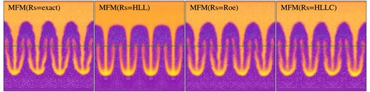
Rayleight–Taylor instability at time t = 3.6, evolved using different Riemann solvers. Secondary instabilities are more or less pronounced, depending on the solver used.
While the instability evolved using the exact Riemann solver shows the most prominent secondary instabilities, closely followed by the Roe solver and the HLLC solver, the HLL Riemann solver leads to a suppression of any asymmetries in the final shape of the instability. This is a result of the additional numerical diffusivity introduced by the Riemann solver, as discussed in Section 4.5.2.
While for specific problems, these alternative solvers could lead to faster results, we in general use the most accurate exact Riemann solver. The increase in runtime is compensated by the gain in accuracy.
APPENDIX C: SOUNDWAVE CONVERGENCE WITH arepo
As described in Section 4.2.1, we would expect Arepo to have better convergence than observed. A first reason is the mesh regularization. If triggered, the position of the cells are shifted, introducing a small numerical noise. In addition, small interfaces which contribute by less than 10−5 to the total interface are neglected. While this makes the code more stable in extreme environments, it introduces small errors (R. Pakmor private communication), which will be relevant for the very small deviations analysed here.
Turning off the mesh regularization and only skipping interfaces which contribute by less than 10−8, Arepo shows much better convergence behaviour, close to what is expected from the analysis by Weinberger et al. (2020), as shown in Fig. C1. Especially, the scatter error drastically decreases, also making the determination of the other error components more reliable.
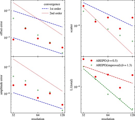
Offset-, amplitude-, scatter and total L1-errors of the density of a soundwave at |$t=\frac{2}{c_s}$|. Applying the changes described in the text reduces especially the scatter error, thus increasing the order of convergence and making also the determination of the other components more reliable. Thus, also the overall order of convergence increases.
While these changes can lead to a better convergence behaviour, they will cause other problems in cosmological simulations, such that in physical applications rather the non-optimized behaviour would be observed.
