


ABSTRACT
We present a study aimed at understanding the physical phenomena underlying the formation and evolution of galaxies following a data-driven analysis of spectroscopic data based on the variance in a carefully selected sample. We apply principal component analysis (PCA) independently to three subsets of continuum-subtracted optical spectra, segregated into their nebular emission activity as quiescent, star-forming, and active galactic nuclei (AGNs). We emphasize that the variance of the input data in this work only relates to the absorption lines in the photospheres of the stellar populations. The sample is taken from the Sloan Digital Sky Survey (SDSS) in the stellar velocity dispersion range 100–150 km s−1, to minimize the ‘blurring’ effect of the stellar motion. We restrict the analysis to the first three principal components (PCs) and find that PCA segregates the three types with the highest variance mapping SSP-equivalent age, along with an inextricable degeneracy with metallicity, even when all three PCs are included. Spectral fitting shows that stellar age dominates PC1, whereas PC2 and PC3 have a mixed dependence of age and metallicity. The trends support – independently of any model fitting – the hypothesis of an evolutionary sequence from star formation to AGN to quiescence. As a further test of the consistency of the analysis, we apply the same methodology in different spectral windows, finding similar trends, but the variance is maximal in the blue wavelength range, roughly around the 4000 Å break.
1 INTRODUCTION
The formation history of galaxies represents a record of the various physical processes that lead to the stellar and gaseous components that we observe at the telescope. In this framework, galaxy spectra encode the kinematics, age and chemical composition of the underlying stellar populations, and thus provide the best available source of information in extragalactic astrophysics. However, retrieving this information is fraught with problems due to the large entanglement of the individual components, preventing us from producing detailed constraints, other than overall estimates such as average ages and metallicities. Over the now long history of stellar population modelling, large advances have been produced (well documented in many reviews, to name a few: Renzini 2006; Walcher et al. 2011; Conroy 2013), and population synthesis models have become commonplace in the analyses of galaxy data (see, e.g. Bruzual & Charlot 1993; Worthey 1994; Fioc & Rocca-Volmerange 1997; Bruzual & Charlot 2003; Maraston 2005; Conroy & Gunn 2010; Vazdekis et al. 2010; Maraston & Strömbäck 2011). The building block of these models is the simple stellar population (SSP), an ensemble of stars that are all formed at the same time, with the same chemical composition, following a well-defined distribution of stellar mass [the so-called initial mass function (IMF)]. Any formation history can be described by a superposition of SSPs, and the resulting photometric and spectroscopic output can be compared with the observations. Three techniques are typically applied to this problem: (1) Model fitting: the spectroscopic information is compared with population synthesis models, whose parameters can be treated in a Bayesian framework, producing estimates of average stellar age, metallicity, abundance ratios, quenching time-scales, etc. (see e.g. Trager et al. 2000; Gallazzi et al. 2005; La Barbera et al. 2014); (2) Machine Learning methods have recently come to the fore, both in a supervised and unsupervised way, with the goal of extracting the kind of information that traditional methods cannot produce (e.g. Ball et al. 2004; Lovell et al. 2019; Portillo et al. 2020; Melchior et al. 2023; Huertas-Company & Lanusse 2023); (3) Multivariate analysis methods can be applied to the spectroscopic data, reducing the problem to blind source separation, making use of data-driven diagnostics such as covariance, clustering, or statistical independence, to overcome the entanglement (e.g. Madgwick et al. 2003; Kaban, Nolan & Raychaudhury 2005; Ferreras et al. 2006; Lu et al. 2006; Nolan, Raychaudhury & Kabán 2007; Rogers et al. 2010b; Wild et al. 2014).
Comparisons with population synthesis models have produced fundamental constraints in galaxy properties, such as the correlation between age or metallicity and stellar mass (e.g. Gallazzi et al. 2005); the increasing [Mg/Fe] in massive galaxies as a signature of rapid formation (e.g. Trager et al. 2000; Thomas et al. 2005; de La Rosa et al. 2011); the differing role of environment in central and satellite galaxies (e.g. Pasquali et al. 2010; Peng et al. 2012; La Barbera et al. 2014); or the presence of small episodes of star formation in early-type galaxies (e.g. Ferreras & Silk 2000; Kaviraj et al. 2007; Salvador-Rusiñol et al. 2020). However, population synthesis methods still produce general results that cannot be taken beyond the lowest order moments of the distributions in age and chemical composition. For instance, quenching time-scales in green valley galaxies determined by direct modelling are still rather vague (e.g. Schawinski et al. 2014; Nogueira-Cavalcante et al. 2018; Angthopo, Ferreras & Silk 2020) and all too often comparable with the typical evolutionary time-scales over which most of the stellar populations vary substantially in the sense of information content (Ferreras et al. 2023). Different spectral fitting codes can produce acceptable solutions with very different formation histories (Ge et al. 2018, 2019).
This paper belongs to probe number 3 in the above list, adopting covariance as the main descriptor of information in galaxy spectra, and making use of principal component analysis (PCA) to understand the main source of variations in the observational data from the Sloan Digital Sky Survey. Furthermore, instead of applying our methodology to synthetic data, we focus on the information content of the observational spectra, in a fully data-driven way. We only use models (e.g. spectral fits to SSPs) a posteriori to give physical meaning to the components statistically derived from the observations. This approach inescapably avoids the prior definition of parameters (e.g. age, metallicity), but, rather, aims at looking for the ‘signal’ present in a carefullty selected sample of spectra. This project is thus complementary to standard techniques, where the goal is to explore at a more fundamental level the limitation of spectral analysis in galaxies.
An important specificity of our work is that we independently apply PCA to three subsets of spectra, classified by their nebular emission into three groups, namely star forming (SF), active galactic nuclei (AGNs), and quiescent galaxies; as explained in Sections 4 and 6. While the input spectra originate from the same data set, a separate analysis allows us to explore the individual properties of these three groups, and to assess the way variance is distributed in the three classes. This new approach to PCA builds upon earlier works that also targeted the spectral energy distribution of galaxies (e.g Yip et al. 2004; Ferreras et al. 2006; Rogers et al. 2007; Portillo et al. 2020; Tous, Solanes & Perea 2020). An additional novelty to our analysis is that the continuum is removed – to focus on the signal from the absorption lines, and spectral windows affected by strong nebular emission lines are removed from the analysis. Moreover, conservative culling is applied to suppress discordant data before determining the covariance matrix in order to fully concentrate on variations caused by the stellar populations (see Sections 2 and 3).
The structure of the paper is as follows: the sample is presented in Section 2, followed by an overview of the methodology in Section 3. The spectral data are decomposed into principal components in Section 4, and the projections are explored in Section 5, along with models of population synthesis. Finally, we discuss the results and present our conclusions in Section 6.
2 SAMPLE
The spectroscopic sample adopted in this paper is taken from the Sloan Digital Sky Survey (SDSS, York et al. 2000). We use the Legacy data set comprising single fibre spectroscopy at resolution R ∼ 2000 (Smee et al. 2013), from Data Release 16 (Ahumada et al. 2020). Systematic effects will be easily picked up by any data-driven method based on variance, so that samples from homogeneous, well-calibrated surveys are essential to avoid spurious results. Moreover, general samples of galaxy spectra will feature a strong variance regarding the well-known correlation of the stellar population properties with stellar mass or velocity dispersion (Bernardi et al. 2003; Gallazzi et al. 2005, 2014; Ferreras et al. 2019b). Therefore, to select a more focused sample, we restrict the stellar velocity dispersion in the range σ ∈ [100, 150] km s−1. We also restrict the redshift to z ∈ [0.05, 0.1] to minimize aperture effects, and impose a threshold on the signal-to-noise ratio (>15 per Δlog (λ/Å) = 10−4 pixel in the SDSS-r band) to reduce the contribution from noise to the variance. The final sample comprises 68 794 spectra.
The spectra were dereddened and deredshifted using a linear interpolation algorithm with redshift and foreground dust estimates supplied by SDSS. Finally, the SEDs were normalized to the same average flux across the 6000–6500 Å rest-frame wavelength range. In this work, we try to minimize as much as possible the potential systematics. Therefore, at the cost of discarding part of the information content of spectra, we remove the continuum. This will allow us to eliminate systematics caused by dust reddening as well as by flux calibration residuals (over similar wavelength scales). We measure the pseudo-continuum with the high percentile method laid out in Rogers et al. (2010a), liberally defined as the boosted median continuum. We adopt a 100 Å running window and a 95 per cent level, an optimal choice for SDSS spectra (see also Hawkins et al. 2014). In addition, once PCA is applied to the data, we explore the standard deviation of the distribution as a function of wavelength to pinpoint problematic data, resulting in a reduced size of the sample, as discussed in detail in the next section. As we explore stellar populations through the variance of the input data, we focus our analysis on the spectral interval 3800–4200 Å – which is the region that keeps most of the information content (see e.g. Ferreras et al. 2023). However, as reference, we also consider the 5000–5400 Å window – that includes prominent Mg and Fe spectral features.
3 PRINCIPAL COMPONENT ANALYSIS
PCA, closely related to the Karhunen–Loève theorem (Karhunen 1947), is a widely adopted multivariate method to explore the variance of large data sets and can be used to classify, compress, denoise data, or to produce a lower dimensional latent space that can be further applied to more sophisticated techniques. PCA rearranges the input data – each defined by N numbers, here the fluxes within a range of N wavelength intervals – into a ranked set of variables, the principal components, by performing rotations in N-dimensional parameter space. These components are defined as those that diagonalise the covariance matrix of the data. Hence, by definition, the principal components are decorrelated – note that, in general, this does not mean statistical independence. A number of papers have been devoted to explore PCA in galaxy spectra (to name a few: Yip et al. 2004; Ferreras et al. 2006; Rogers et al. 2007; Portillo et al. 2020; Tous et al. 2020).
In a nutshell, PCA reduces to the diagonalization of the covariance matrix, where the eigenvalues represent the individual contribution to the variance of the eigenvectors (also known as principal components). These are ranked in decreasing order of variance, typically given as the fractional contribution, producing the so-called scree plot (fractional variance versus rank), that gives a graphical representation of how higher order components contribute progressively less towards the total variance. Projecting the spectra on to the eigenvectors produces the ‘coordinates’ in latent space, and the first few components are expected to keep most of the information, in the sense of variance. Although PCA is mostly used for classification purposes (e.g. Folkes, Lahav & Maddox 1996; Madgwick et al. 2003; Nersesian et al. 2021), in this study, we target instead how the latent space encodes differences in the underlying stellar populations of different groups of galaxies. More information about this approach to PCA in galaxy spectra can be found in Ferreras et al. (2006) and Rogers et al. (2007, 2010b). The samples in those papers focused on quiescent, early-type galaxies, whereas the present work does not introduce such a restriction, including SF and AGN galaxies in the analysis.
One can interpret a spectrum as a vector in a high-dimensional space spanned by a set of wavelengths (λi, i = {1, ⋅⋅⋅, N}). Therefore, the fluxes corresponding to the k-th galaxy in a sample (Φk(λi), k = {1, ⋅⋅⋅, M}) are the coordinates in the space spanned by unit vectors |$\hat{\lambda }_i$|. Our aim is to derive a lower-dimensional set of vectors that are representative of a large sample of galaxy spectra, so that the reduced set of components encapsulates most of the variance in the ensemble. The fundamental element in this method is the difference between the flux of a spectrum, say for the kth galaxy, and the mean at a given wavelength (λi):
where 〈⋅⋅⋅〉s represents averaging the quantity inside the brackets, with respect to the sample of (s = {1, ⋅⋅⋅, M}) galaxy spectra. The covariance is defined as follows:
This is an N × N symmetric, positive-definite matrix. We note that the covariance is sensitive to the presence of outliers – an equivalent case is least-squares fitting a set of data points to some model function. To produce a more robust covariance, we apply a conservative culling process, where spectra are removed if the following condition applies:
where σ(λi) is the standard deviation of the distribution of fluxes at a given wavelength. Note this condition is enforced at all wavelengths in the spectral region of interest. Therefore, the adopted culling process is rather aggressive but ensures that our PCA results are safely driven by the underlying variance of the data and not by the presence of outliers. To diagonalize the covariance matrix, we need to solve the eigenvalue problem, that involves finding a matrix |${\cal U}$|, such that:
where Π is a diagonal matrix containing the eigenvalues of |${\cal C}$|, and |${\cal U}$| contains the eigenspectra (or principal components), e.g.:
with πk representing the eigenvalues (i.e. the variance associated to the kth principal component). Now we can project the observed spectra on the |$\lbrace \hat{e}_k\rbrace$| vectors to obtain the ‘coordinates’, eigencoefficients, or – overloading notation – ‘principal components’. Therefore, we now have two alternative representations of a galaxy spectrum: the traditional one, given by the fluxes, {Φ(λi)}, or the principal component projections, {PCk}. The advantage of the latter is that we can restrict the description to the first few components and still keep most of the original variance of the data set. Note that, similarly to least-squares fitting, PCA is overly sensitive to outliers – the former indeed minimizes the variance between the data and some fitting function. Therefore, it is very important to ensure the input data are free from systematics, hence the careful definition of the sample presented in the previous section. For instance, galaxy spectra will be affected by emission lines from the diffuse gas, and spectra with very intense emission lines (as in star-bursting galaxies or strong AGN), will disproportionately affect the first few principal components, biasing the analysis. Our goal is to assess differences concerning the stellar populations, leading us to avoid a few spectral windows with prominent emission lines that may dominate the variance. Rather than masking the regions, we completely remove these spectral intervals when computing the covariance matrix.
4 DECOMPOSITION OF SDSS SPECTRA INTO PRINCIPAL COMPONENTS
To explore the stellar populations of different groups of galaxies through the variance of the input data, we focus our study on two spectral intervals. These intervals keep most of the variance from galaxy to galaxy (see e.g. Ferreras et al. 2023). The dominant region is roughly centred on the 4000 Å break, between 3800 and 4200 Å. This region features a large number of absorption lines that strongly depend on the age and chemical composition of the underlying populations (see e.g. Bruzual & Charlot 2003). The second interval is defined between 5000 and 5400 Å and mainly focuses on the Mg–Fe complex, a region often used to constrain chemical abundance. Throughout this paper, we will refer to these two spectral regions as the ‘blue’ and ‘red’ interval, respectively. Fig. 1 shows the median (top) and standard deviation (bottom) of the continuum-subtracted spectra, segregated into quiescent (Q), SF, and AGN, as labelled, in the blue and red intervals. Note the contribution to the variance of the most prominent emission lines: 3869 Å([Ne iii]); 3889 Å(Hζ); 3969 Å(Hϵ), and 4100 Å(Hδ), in the blue interval, and 5007 Å ([O iii]) in the red interval, shown as grey shaded regions. Since these lines originate in the diffuse gas, we remove the spectral windows from the covariance matrix. The reason for removing these regions can be seen in the standard deviation plot of Fig. 1, the emission lines feature strong variations among galaxies. Such a signal would be picked up by PCA as a source of information or variance and influence our analysis. The size of the avoided regions is chosen so as to fully eliminate the contribution of the emission lines, as shown in Fig. 1. We emphasize that our aim is to avoid any source of variance unrelated to the stellar content, not to achieve a level of completeness. The remaining spectral features contributing to the variance originate in the stellar atmospheres and show up as absorption lines.
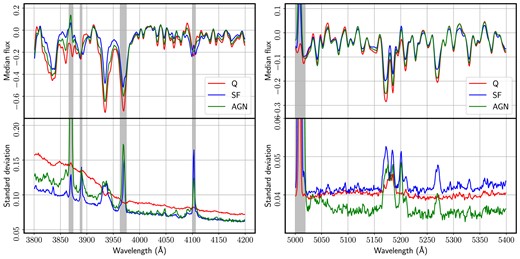
Median (top) and standard deviation (bottom) of the SDSS continuum-subtracted spectra used in this paper (including a 4σ cull of the input data), segregated with respect to nebular activity into quiescent (Q), SF, and AGN. The grey shaded regions represent the intervals removed from the analysis.
While the rest-frame NUV region contributes a rich selection of population sensitive absorption lines (e.g. Vazdekis et al. 2016), we do not consider it, as the S/N of SDSS spectra drops blueward of λ ≲ 3800 Å, heavily affecting any variance analysis. At the red end, the variance of the absorption lines beyond 5400 Å is substantially lower. However, we show further below a comparison of these two spectral intervals with an additional third one, 5800–6200 Å, to illustrate the consistency of our analysis. We do not extend the analysis beyond 6200 Å, so as not to be affected by the strong lines Hα and [N ii] emitted by the diffuse gas. Note that airglow emission lines might introduce prominent residuals in individual spectra, however our working sample covers quite homogeneously a wide range of redshifts, thus minimizing the chance of sky emission lines affecting the combined analysis (see Appendix A). It is worth noting that PCA can be alternatively applied in the observer frame, to remove the contribution from airglow (Wild & Hewett 2005).
The SDSS spectra has been classified with respect to nebular emission into SF, AGN, and quiescent galaxies, making use of the standard BPT line ratio diagnostics (Baldwin, Phillips & Terlevich 1981). While our analysis strives to eliminate the contribution from dust and gas, the BPT classification has a further hypothetical interpretation as an evolutionary transition from star formation towards quiescence (see e.g. Schawinski et al. 2007; Angthopo, Ferreras & Silk 2019). We bin the galaxy spectra according to this criterion to focus our analysis on three separate stages of galaxy evolution. Hence, we define three independent covariance matrices corresponding to spectra classified as SF, AGN, and quiescent (Q). We emphasize that PCA is a powerful data-driven technique that efficiently detects the different contributions of variance. However, it is rather sensitive to the presence of outliers, and thus prone to systematics if the sample is not chosen carefully. If we apply PCA to the whole sample, i.e. with a single covariance matrix, it will pick a larger signal caused by the trivial difference between galaxies of different types. We would like to focus instead on variations within each group, and then among the three classes. In this way, it is possible to find in a robust way systematic differences between the stellar populations in different groups of galaxies. The BPT classification is taken from the official galspecExtra SDSS catalog from the MPA-JHU group (Brinchmann et al. 2004). Regarding quiescent galaxies, we select those with a BPT flag of −1, along with a threshold on the equivalent width of Hα emission, analogously to Cid Fernandes et al. (2011). The SF sample adopted in the analysis is restricted to BPT flag 1 (i.e. excluding low star-forming galaxies), and the AGN sample is also restricted to BPT flag 4, therefore excluding LINERs. The sample is reduced from 68,794 to 37,006 spectra.As explained in Section 3, during the calculation of robust covariance matrices, we remove outliers in each subgroup by culling the samples at the cost of reducing their sizes. In the 3800–4200 Å spectral interval the number of galaxies is reduced from 23 168 to 17 473 (Q); from 10495 to 8025 (SF), and from 3343 to 2620 (A). In the 5000–5400 Å spectral interval, the samples are reduced from 23 168 to 13 953 (Q), from 10 495 to 6319 (SF), and from 3343 to 2019 (A). Finally, to ensure that our results do not depend on the numerical solver, we tested different methods to diagonalize the covariance matrix. We applied python-based codes from scikit-learn (decomposition.PCA) and from the linalg package (eig and svd). All three gave undistinguishable estimates of the eigenvalues and eigenvectors.
Fig. 2 shows the scree plot corresponding to the three different sets in the blue (left) and red (right) spectral window, colour-coded as labelled. In all cases, the steepness of the scree plots confirms the dominance of the first few principal components. It is worth noting that in both choices of wavelength window, AGN spectra have a higher fraction of total variance in the first component with respect to SF or Q. We also note the contrast in these scree plots with analyses based on full spectra (i.e. including the continuum), where, for instance, early-type galaxies include over 90 per cent of total variance in the first few components (see e.g. Rogers et al. 2007). Removing the continuum makes the data less compressible. In our sample, performing the same analysis in the blue interval on data without continuum subtraction results in a fractional variance of the first principal component of 73 per cent (AGN); 84 per cent (SF), and 36 per cent (Q), in marked contrast to our adopted, continuum-subtracted, spectra, for which the contribution of the first component is 12 per cent (AGN); 8 per cent (SF), and 3 per cent (Q) of total variance. This confirms the continuum encodes a large amount of variance, or information. However, our approach is aimed at minimizing all potential systematics, and dust can produce substantial entanglement with respect to variations in the underlying stellar populations. In principle, the higher-order components will be more severely affected by noise, but this interpretation is not straightforward, and truncating the PCA decomposition to denoise spectra is a far from trivial task. The blue interval keeps a higher ratio of the variance in the first component (∼10 per cent) with respect to the red interval (∼5 per cent), which is perhaps indicative of a higher level of correlatedness at bluer wavelengths (i.e. higher compressibility). In absolute terms, the blue interval has substantially higher variance: for instance, AGN spectra have absolute variance of 0.357 in the first component for the blue interval, and 0.036 in the red interval. This paper focuses on the lowest order components of variance, so we will restrict the analysis to the projections of the data on to the first three principal components.
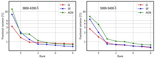
Scree plots showing the first eight eigenvalues of the PCA decomposition performed in the blue (left) and red (right) spectral intervals. The sample is split regarding nebular emission activity into quiescent (red, Q), star forming (blue, SF), and AGN (green), as labelled.
The first three eigenspectra of the SF (blue), AGN (green), and Q (red) galaxies are shown in Fig. 3 in both spectral windows (left-hand/right-hand panels). The vertical grey shaded regions correspond to the intervals removed from the analysis. We note that the covariance matrix is sign invariant, i.e. a change in the sign of a principal component (and thus its projections) does not affect the matrix. Therefore, the comparisons between the three covariance matrices can be affected by a sign change. To mitigate this issue, we enforce a positive sign for the median of the projections of all galaxies of the corresponding type. When restricting to the first three principal components, this means the data are statistically constrained to the first octant of the latent space spanned by the 3-tuple {PC1, PC2, PC3}.
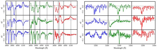
Principal components of the three subclasses, namely SF (blue), AGN (green), and quiescent (red). The left-hand (right-hand) panels correspond to the results produced by the blue (red) spectral interval. The vertical grey shaded regions correspond to the intervals removed from the analysis.
5 PROJECTING THE DATA ON TO THE PRINCIPAL COMPONENTS
Once we have set the three eigenspectra with the highest variance as those that encapsulate most of the information regarding absorption lines, we project the SDSS spectra on to those, separated with respect to their classification as SF, AGN, or Q. For instance, principal component number one for the jth galaxy is defined as:
where N is the total number of wavelength bins in the spectrum. We note that we only present the projected sample that have not been rejected by the condition described in equation (3), although the results do not vary significantly if the full sample is considered instead. Each spectrum is thus simplified by three ‘coordinates’, namely PC1, PC2, and PC3 and can be visualized in a three-dimensional latent space. We emphasize that the results are obtained from continuum-subtracted spectra, rejecting regions dominated by nebular emission lines, so that the analysis does not depend on the dust or gas components.
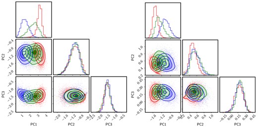
Fig. 4 shows the latent space of the SDSS galaxy spectra, in blue (SF), green (AGN), and red (Q), in both spectral windows: blue (left) and red (right). We use the publicly available python code of Foreman-Mackey (2016) to produce a visual representation of the distributions in the three components with the so-called ‘corner’ plots. The 2D projections are shown as a colour scale mapping the number density of points at a given position. The most salient feature is that the spectra are projected in separate regions of their respective latent spaces, regarding their nebular emission properties. We emphasize that although the figure shows projections onto different eigenvectors, depending on their nebular activity classification, the underlying data concern one and the same component, namely the stellar populations of the galaxies (after careful removal of features affected by dust or ionized gas). Therefore, Fig. 4 is not a disjoint comparison of PCA projections, and the eigenvectors of the three groups are not completely independent. The three sets of eigenvectors reflect, instead, the typical stellar populations found in each group. The separation between the three subgroups found in the figure is reminiscent of the bimodal distribution into blue cloud (i.e. SF) and red sequence (i.e. quiescent) galaxies (e.g. Strateva et al. 2001; Baldry et al. 2004), with AGN preferentially populating the green valley (see e.g. Schawinski 2012; Salim 2014; Angthopo et al. 2019). The separation is more pronounced in the blue interval, where both PC1 and PC2 show clear separation between the three groups, with AGN located in between the other two. PC3 puts SF and Q galaxies together, and AGN standing out with higher values. In the red interval, the distributions also appear separately when projected on to PC2, whereas PC1 appears to ‘isolate’ Q galaxies and PC3 sets AGN aside. To help visualize the distribution of principal component projections, we show in Fig. 5 a rotating animation of the 3-dimensional latent space. Note that while PCA is independently applied to three different covariance matrices, which results in different eigenvectors, their clustering is significant even considering the different orientations. Given the input data lack, by construction, emission lines of even continuum, the clustering is representative of the variations in the stellar population content. These figures also illustrate one of the biggest problems encountered in a data-driven, multivariate approach: it is very difficult to ascribe such differences to specific physical/observational factors. The eigenvectors in Fig. 3 have some physical features but they cannot be associated, say, to specific populations, or phases of evolution. Therefore, to gain more insight of the meaning of these projections, we show in Figs 6 and 7 the way these projections depend on a number of observable properties. In each panel, we separately sort each subsample (Q, SF and AGN) in increasing order of the PC1, PC2 or PC3 projection, and show the running median – choosing bins that encompass 1/20th of each subset, therefore comprising from 100 to over 800 galaxies per bin – along with the 1σ uncertainty of the median, shown as a shaded region. We follow the same colour coding as above. The panels on the left trace more general observables, from top to bottom: stellar velocity dispersion in units of 100 km s−1; stellar mass (measured as |$\log \,$|M/M⊙); surface stellar mass (log Σs); and volume stellar mass (log ρs). The last two are defined as Σs ≡ Ms/R|$_P^2$|, and ρs ≡ Ms/R|$_P^3$|, respectively, where Ms is the total stellar mass in solar units and RP is the Petrosian radius in the SDSS-r band, measured as a projected physical distance at the redshift of the galaxy, in kpc. The panels on the right show spectroscopic measurements, from top to bottom: Mgb; average Fe = 0.5(Fe5270 + Fe5335) (Trager et al. 1998); Dn(4000) (as defined in Balogh et al. 1999), and HδA (Worthey & Ottaviani 1997). These estimates are all derived from the official SDSS catalogues. The results are presented for the blue interval (Fig. 6) and the red interval (Fig. 7). We emphasize that these projections concern continuum-subtracted data without any contribution from emission lines. Therefore, the associated variance is independent of the dust and gas components.
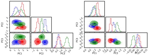
Distribution of the projections of the galaxy spectra on to the first three principal components, colour-coded as SF (blue), AGN (green), and quiescent (red).The left-hand (right-hand) panels correspond to the results produced by the blue (red) spectral interval. The contours engulf 25 per cent, 50 per cent, 75 per cent, and 90 per cent of each subsample. See Fig. 5 as complement to this figure.
Animated version of the distribution of the projections of a representative sample of galaxy spectra on to the first three principal components. The data are colour-coded as SF (blue), AGN (green), and quiescent (red). The top (bottom) panels correspond to the results produced by the blue (red) spectral interval. The framed structure represents a sphere with radius 1 and is only shown for reference. There is a version with animated figures), with the following (using LaTeX + hyperref) An animated version of the figures can be found at https://cloud.iac.es/index.php/s/firKQ2BFkC7xzSf (for the blue interval) and https://cloud.iac.es/index.php/s/deniTo6SgpiBsR4 (for the red interval).
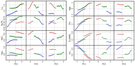
Correlation of the projections on to the first three principal components with observable features of galaxies in the blue spectral range (3800-4200 Å). In each panel, the data are shown separately for quiescent (red), SF (blue) and AGN (green), as a running median towards increasing values of the PC1, PC2, and PC3 projections. The shaded regions mark the 1σ uncertainty of the median. See text for details.
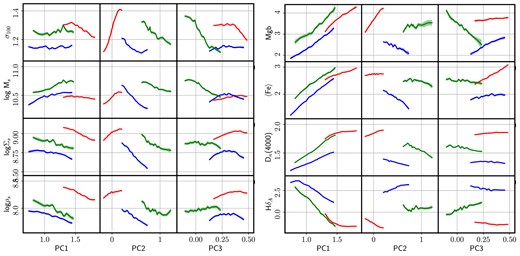
Equivalent of Fig. 6 for the analysis of the red spectral interval (5000–5400 Å).
The figure shows a strong correlation of PC1 with all spectral observables, unsurprisingly, given that PCA produces the components based on the variance of the data, which reduces to the absorption lines. However, it is rather unexpected to find the much weaker dependence of the higher order projections PC2 and PC3. The scree plot indicates a substantial fraction of total variance in these components; nevertheless, they appear not to correlate so strongly with the spectral data. The red interval produces similar results, but Mgb and 〈Fe〉 feature a sizeable correlation with PC2 and PC3, with respect to the blue interval. It is a well-known fact that all spectral indicators are deeply entangled, i.e. the so-called age-metallicity degeneracy (Worthey 1994; Ferreras, Charlot & Silk 1999) has a deeper version when considering the covariance among different spectral indicators (see figs 10 and 11 of Ferreras et al. 2023). Regarding the general observables (left-hand panels), both blue and red intervals display a strong correlation with velocity dispersion. The relation between σ and PC2 is stronger in quiescent galaxies, and especially in the red interval. These galaxies tend to have stronger absorption features (see Fig. 1), and the Mgb–Fe region is optimal to measure velocity dispersion. However, it is noteworthy that this signal (roughly the width of the absorption lines) is listed by PCA as the second-largest variance, with the depth of these features ranking higher – i.e. the trend of PC1 with the line strengths. Stellar mass and surface/volume densities also correlate with the projections, but we conclude that this trend is inherited by the relation with σ, as this parameter strongly correlates with both. We should emphasize here that this sample extends over a relatively small range of velocity dispersion – on purpose, to avoid ‘distracting’ the variance with the well-known age-mass and metallicity-mass correlations (e.g. Gallazzi et al. 2014). Nevertheless, the data clearly display a version of these scaling laws over the narrower range of mass and velocity dispersion.
It is also worth mentioning that these trends are followed in different ways in Q, SF, and AGN spectra, especially in the higher order (i.e. lower variance) projections. The most evident discrepancy between these subclasses is average age, and perhaps chemical composition, but more subtle differences might be due to details of the underlying stellar populations.
5.1 Projection of simple stellar populations
The trends of the principal component projections shown in Figs 6 and 7 have been obtained in a model-independent way. Therefore, they are free of the inherent systematics caused by comparisons with models that suffer from degeneracies. However, we cannot give physical meaning to those. We now turn to stellar population synthesis, with the aim of translating those trends into parameters that describe, to the lowest order, the properties of the stellar component. We first produce SSPs from the MIUSCAT models (Vazdekis et al. 2012) for a range of ages (0.1<tSSP <14 Gyr), at three different metallicities: [Z/H] = {− 0.4, 0, +0.22}, with a fixed stellar IMF (Kroupa 2001). The SSP spectra are convolved to the mean velocity dispersion of the observed galaxies, and resampled to the same wavelength binning. Moreover, following the same methodology as with the SDSS data, we remove the pseudo-continuum. While these population synthesis models do not include nebular emission from diffuse gas, we also remove the regions contaminated by emission, for a consistent analysis. Finally, we project the processed spectra onto the principal components obtained from the analysis, showing the synthetic data as three separate age tracks in Fig. 8, one for each choice of metallicity (solid lines for solar metallicity, dotted for super-solar, and dashed for subsolar metallicity). For reference, the oldest population is shown as a symbol (star, circle, and cross for solar, super-solar, and subsolar metallicity, respectively). Note that there are three separate sets of tracks as we project the SSP spectra on to the principal components from the Q (red), SF (blue), and AGN (green) covariance matrices. For reference, we also show as a contour plot, the number density of observed spectra (each contour encompases, from the inside-out, 50 per cent, 75 per cent, and 95 per cent of the data). The left-hand (right-hand) panel corresponds to the analysis in the blue (red) interval. Fig. 9 is an animated 3D version of the projections shown in Fig. 8, using a representative sample of 100 data points, selected randomly from each subset.
![Projection of SSPs from the MIUSCAT models (Vazdekis et al. 2012) on to the first three principal components. The age ranges from 0.1 to 14 Gyr, the oldest one represented by a symbol, with metallicity [Z/H] = −0.4 (dashed), 0.0 (solid), and +0.22 (dotted). For reference, the number density of the SDSS sample is shown as contours engulfing 50 per cent, 75 per cent, and 95 per cent of each subset. The colour coding is the same as in Fig. 4. The left-hand (right-hand) panels correspond to the results produced by the blue (red) spectral interval.](https://oup.silverchair-cdn.com/oup/backfile/Content_public/Journal/mnras/526/1/10.1093_mnras_stad2668/1/m_stad2668fig8.jpeg?Expires=1750088580&Signature=SCl3ZdUb1fpbuL7X9yoA8WxjsoQfX60ezglPEqWyeT06esUiRMBCKGYNWGOuik7QAfgtEYZUwljqXRi4nlrVH-EfqYc3hLcw208Hu8M3qHj5q7uoKZPK3gS5asotDQ0hgQOwUHVdlJGb3-jNCpddCf2rhR4aCmFNLQhFXbaJ~HbLNgW~iWcLrdrWZVGb9Cwb9APIwSKaHgcJRLTaTcfjwibAFSq8dr2jcIkpyAH1tYJNHmx-i2fkXmDseNHOXwnW4JLVMijQfzzCSd5441QypKVVqdYZQZ6GWxExBq4fyM-9ge5FM-LEIgdYDqBX5fA1Acz3V8fBesdYpNJ30K-Xtg__&Key-Pair-Id=APKAIE5G5CRDK6RD3PGA)
Projection of SSPs from the MIUSCAT models (Vazdekis et al. 2012) on to the first three principal components. The age ranges from 0.1 to 14 Gyr, the oldest one represented by a symbol, with metallicity [Z/H] = −0.4 (dashed), 0.0 (solid), and +0.22 (dotted). For reference, the number density of the SDSS sample is shown as contours engulfing 50 per cent, 75 per cent, and 95 per cent of each subset. The colour coding is the same as in Fig. 4. The left-hand (right-hand) panels correspond to the results produced by the blue (red) spectral interval.
Distribution of the projections of a representative sample from each of the three subsets onto the first three principal components, along with the corresponding projections of SSPs from population synthesis models. The data are colour coded as SF (blue), AGN (green), and quiescent (red). The results for the blue (red) spectral interval is shwn in the top (bottom) panels. The framed structure represents a sphere with radius 1, and is only shown for reference. There is a version with animated figures with the following (LaTeX+hyperref source): An animated version of the figures can be found at https://cloud.iac.es/index.php/s/HDcQftPJsYFEoxG (for the blue interval) and https://cloud.iac.es/index.php/s/7Q2NEBnEQ3PWAYM (for the red interval).
The most noticeable result of this comparison is the strong age dependence of PC1, in both spectral intervals. In the red interval PC2 and PC3 also have a monotonic trend with age, whereas in the blue interval the higher order components have more subtle variations, with PC2 changing only for younger ages (similar to, e.g. Balmer absorption), and PC3 has a substantial correlation with age only for the SF subsample.
Regarding metallicity, these projections illustrate in a remarkable way the fundamental nature of the age-metallicity degeneracy. In this 3D latent space, the effect of changing metallicity is equivalent to a change in age, as the tracks at different metallicity simply ‘slide’ with respect to each other, in the expected direction that increasing metallicity produces an equivalent effect as an increase of age. We emphasize the importance of this result, as the traditional case is based on photometric and spectroscopic observables (e.g. Ferreras et al. 1999), whereas this result depends at the most fundamental level on the intrinsic variance of stellar population spectra. Finally, we note the acceptable agreement between synthetic spectra and real galaxies, except for the case of quiescent galaxies in the red interval, where the synthetic tracks do not overlap the bulk of the observations. As this region is dominated by the Mgb–Fe complex, we suggest this discrepancy may be due to non-solar abundance ratios, more prevalent in quiescent galaxies (e.g. Trager et al. 2000; Kuntschner et al. 2010).
5.2 Spectral fitting of projected data
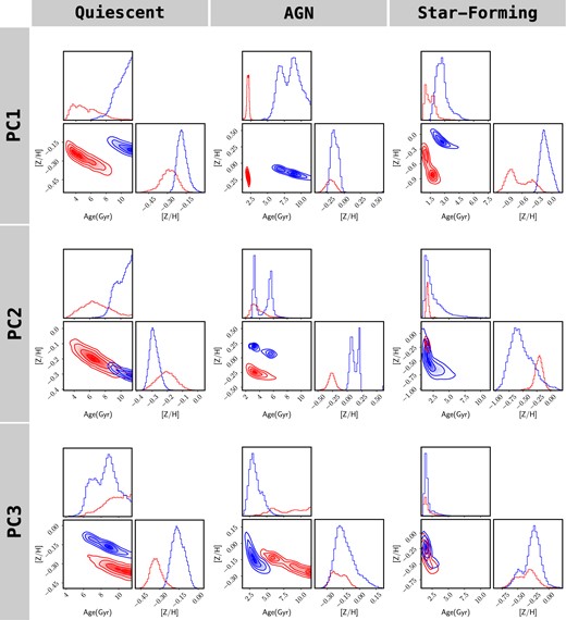
Building upon the previous comparison of synthetic data projected on the latent space generated by the real spectra, we now make a more standard analysis by stacking spectra within a given (SF/AGN/Q) subclass regarding their projections. For each choice of the spectral interval and nebular emission type, we produce two stacked spectra, combining the data from galaxies in the 10th and 90th percentile of the distribution of each principal component. The resulting stacks are then compared with SSPs using a standard method based on the χ2 statistic, fitting the continuum-subtracted data – for consistency with our analysis, the continuum does not play any role in the fitting – and adopting the standard likelihood |${\cal L}(t,[Z/H])\propto \exp (-\chi ^2(t,[Z/H])/2)$|, where the only two parameters considered are the age (exploring the 0.01–11.5 Gyr range) and total metallicity (between [Z/H] = −2.3 and + 0.2) of the SSP (keeping the stellar IMF of Kroupa 2001). We adopt the python-based MCMC solver emcee (Foreman-Mackey et al. 2013) to produce the confidence levels of the fits, shown in Fig. 10. The contours are shown at the 1, 2, 3, and 4σ levels, with the lowest PC projections in red (10th percentile) and the highest in blue (90th percentile). The columns, from left to right, represent Q, AGN, and SF spectra, and the rows, from top to bottom, correspond to the distribution of PC1, PC2, and PC3 projections. We use the same population synthesis models as in Fig. 8.
![Confidence levels of the SSP-equivalent age (in Gyr) and metallicity ([Z/H]) obtained from fitting the spectra (continuum subtracted) with the MIUSCAT population models (Vazdekis et al. 2012). We fit the stacked spectra with the lowest (10 percentile, red) and highest (90 percentile, blue) value of PC1, PC2, and PC3 (from top to bottom), for Q (left column), AGN (middle column) and SF galaxies (right column). The principal components obtained correspond to the covariance defined in the blue interval.](https://oup.silverchair-cdn.com/oup/backfile/Content_public/Journal/mnras/526/1/10.1093_mnras_stad2668/1/m_stad2668fig10.jpeg?Expires=1750088580&Signature=2TGOQTKzeQcT5VCQKw8BzRixrVflW9fo-dj-NtMFSnTQRAJgr~cpN~n0aWS~5o~U~bLfgv8bcszZlYhK7ZJCMkKHgJ-ELYiZAxKoEWrj054JMJPrE3yt~uj~HlHas91Nav0DLJI9zGWSJg7hBNmRifB8i0kcwh-hsSpy-Io-zgsDBDZbQQm5hSd1rAFVi3uoGjlDBv7kwPJkeX~2DUTlGtdXIKAwbLeG7~5NBHTGl76liHUaCoaAEXsmfqnuwE23SK5gS03bEpSsVrxGm~sq5oGaICobIfur5pqzAywFxkkyU6S5VmAFwYZRAl-qN5OTCsPbB0Z6rnAmFqFb0ZruQA__&Key-Pair-Id=APKAIE5G5CRDK6RD3PGA)
Confidence levels of the SSP-equivalent age (in Gyr) and metallicity ([Z/H]) obtained from fitting the spectra (continuum subtracted) with the MIUSCAT population models (Vazdekis et al. 2012). We fit the stacked spectra with the lowest (10 percentile, red) and highest (90 percentile, blue) value of PC1, PC2, and PC3 (from top to bottom), for Q (left column), AGN (middle column) and SF galaxies (right column). The principal components obtained correspond to the covariance defined in the blue interval.
Consistently with the projected tracks, we find that the highest/lowest values of PC1 correspond to the oldest/youngest galaxies, respectively, in all three subgroups, with the average populations being, unsurprisingly, younger in the sequence Q→AGN→SF. No significant difference is found with respect to metallicity in Q and AGN, whereas SF stacks also show different metallicities in an opposite direction to the age-metallicity degeneracy (the latter tracing the elongated confidence levels, from top left to bottom right in these plots). This may be caused by the fact that the degeneracy is usually more entangled in older populations. PC2 produces mixed results: Q spectra do not show any appreciable difference, AGN galaxies reveal a correlation with metallicity, towards high PC2 projections having a higher [Z/H], and SF may just show a mild correlation with age, with the low PC2 distribution hinting at a tail towards older ages. PC3 behaves similarly to PC2 in Q and SF galaxies and anticorrelates with metallicity in AGN spectra. Appendix B shows the confidence levels as in Fig. 10 for the red spectral interval. The trends are strongly consistent for the projections on the first principal component, reflecting the substantial covariance across a wide range of spectra wavelengths (as illustrated in Ferreras et al. 2023). The comparison is more subtle with PC2 and PC3. For instance, PC2 keeps a positive correlation in AGN with respect to metallicity.
6 DISCUSSION AND CONCLUSIONS
The focus of this paper is to explore galaxy spectra by relying exclusively on the data to extract information about the underlying stellar populations. This approach is complementary to standard methods based on population synthesis modelling (see e.g. Cid Fernandes et al. 2005; Tojeiro et al. 2007; Cappellari 2012; Wilkinson et al. 2017; Robotham et al. 2020). The ‘front end’ of these models depend on a small set of parameters that allow a relatively simple fit of photometric and spectroscopic observations. These parameters relate to the age, metallicity, chemical enrichment, star formation, or stellar mass. The model-based studies are limited due to the high entanglement and complexity in the definition of parameter space, with a number of strong degeneracies, such as the one between age, metallicity, and dust (Worthey 1994; Ferreras et al. 1999). In this study, as explained in Section 3, we adopt a multivariate analysis method, PCA, as a blind source separation technique to decipher the information encoded in the optical spectra of ~37000 galaxies from the Legacy part of SDSS. We only use population synthesis models a posteriori, to gain physical insight of the components retrieved by the statistical analysis.
As the analysis is purely dependent on the input data, we need to make sure the spectra have a high enough signal-to-noise ratio, and, most importantly, we remove the pseudo-continuum and avoid spectral intervals dominated by emission lines, so that the contribution from dust and diffuse gas is minimized. At the same time, we need to focus the data as much as possible to avoid being overwhelmed by well-known trends, such as the age–mass and metallicity–mass relations (e.g. Gallazzi et al. 2005), or by the effect of stellar velocity dispersion on the effective resolution of the spectra. Therefore, we also restrict the sample to relatively low velocity dispersion (σ ∈ [100, 150] km s−1). Moreover, we split the sample into three subsets, according to the nebular emission properties into quiescent, AGN and SF, noting, though, that the input data do not include the flux from emission lines, so that the observed variance only depends on the absorption lines originating in the atmospheres of the stellar populations. Concerning variations in the stellar IMF, such as the observed bottom-heavy phase in the cores of massive early-types (e.g. van Dokkum & Conroy 2010; Ferreras et al. 2013; La Barbera et al. 2019) or a top-heavy phase in SF galaxies (e.g. Lee et al. 2009; Gunawardhana et al. 2011), we emphasize that our sample is representative of a general, relatively low-mass population, for which a standard IMF gives a good representation. Note also that the signatures typically found in absorption-line spectra from IMF variations stay at the sub- per cent level (see e.g. La Barbera et al. 2013).
Previous work applying PCA to galaxy spectra finds a high compressibility, showing, for instance, that over 90 per cent of the total variance is encoded in a single principal component (Rogers et al. 2007). However, our data (Fig. 2) show a more spread distribution of the weights, which reflects the high level of correlatedness of the pseudo-continuum, that is removed in our analysis. In our data, the first component holds up to ∼10 per cent of total variance, where Q galaxies have the lowest variance. This is a reflection of the fact that quiescent galaxies have a more homogeneous distribution of (older) populations, but it is noteworthy to compare SF and AGN subsets, with the latter consistently keeping a higher fraction of variance in both spectral windows.
By projecting the observed spectra on to the first three principal components, we reduce the dimensionality of the problem, describing each galaxy by a set of three numbers that keep the highest amount of variance. Our aim is to understand how these components relate to physical properties. The trends shown in Figs 6 and 7 show that the first component is strongly correlated with traditional spectral indicators (4000 Å break strength, Balmer lines and Mg and Fe absorption). However, in the higher-order components, the trend is less trivial. For instance, PC3 cleanly separates AGN from the other galaxies in both spectral intervals (see Fig. 4), with milder trends with respect to the line strengths, except for HδA in SF galaxies for the blue interval and Mgb in AGN + SF, as well as 〈Fe〉 in Q for the red interval. The distribution of PC2 projections feature the largest separation between the three subsets Q/AGN/SF in both spectral intervals, and have mixed behaviour regarding the trends with the line strengths. Turning to the other parameters, a trend is found with velocity dispersion, which can be caused by a combination of a physical correlation, as σ traces the gravitational potential of the galaxy and hence its formation history, but there is also an instrumental effect, as σ will affect the effective resolution of the spectra. We cannot ascribe any of these parameters as major drivers of evolution, similarly to traditional work (Ferreras et al. 2019b)
Projecting synthetic spectra of SSPs, as shown in Figs 8 and 9, confirms that PC1 in both spectral intervals strongly correlates with stellar age. It is worth mentioning that PC2 – that clearly separates the three types – is more entangled with SSP parameters, with the red interval PC2 showing monotonic behaviour with age, but the blue interval PC2 featuring a more complex evolution, with a characteristic kink at young ages. PC3 is even less predictable from an SSP based analysis. The SSP tracks also provide an excellent illustration of the age-metallicity degeneracy. Population synthesis models have already shown this entanglement (e.g. Worthey 1994; Ferreras et al. 1999), but the variance analysis gives a more robust visualization, so that changes in either SSP-equivalent age or metallicity evolve very much in the same direction, even up to the third principal component. This is a sobering reminder of the difficulty in extracting information from galaxy spectra.
We also performed spectral fits to stacked data based on the highest and lowest percentiles of the distribution of PC1, PC2, and PC3 (Fig. 10). PC1 consistently maps SSP-equivalent age in the three subsets, and PC2 and PC3 show a mixed dependence with respect to the SF/AGN/Q nature of the galaxy. Q galaxies appear not to feature any substantial difference with respect to high/low values of PC2 and PC3. AGN galaxies have a significant trend in PC2 and PC3 with metallicity, and the SF subset show high overlap of the parameter distribution, but with a hint of a tail in the probability distribution towards older ages in galaxies with the lowest projections. Our PCA decomposition fully depends on absorption lines (neither continuum nor emission lines are included), and aligns with the hypothesis of AGN statistically representing a transitioning phase between star formation and quiescence (Schawinski et al. 2007). This work, however, cannot reject the hypothesis of a quenching channel purely driven by star formation. We emphasize that these three components are based on a variance analysis of observational data. However, the idiosyncrasy of PCA, for instance, the enforced orthogonality of the eigenvectors, may result in unphysical components. The way forward, reserved to future work, will involve comparisons with realistic models of galaxy formation and evolution (Sharbaf et al., in preparation).
The inquisitive reader might ponder about the way we separated the sample in three sets, producing three different covariances. The motivation is to maximize the ability of PCA to retrieve a meaningful signal. By putting all the galaxies together, we produce a more mixed population where the first few components will be most sensitive to the mixture. However, we include another test by diagonalizing a single covariance, i.e. putting together the whole sample regardless of the SF/AGN/Q nature. In addition, we do not cull the sample according to equation (3) and show the projections in Fig. 11, where the colour-coded separation is performed after the diagonalization, i.e. there is a single set of eigenvectors. Note PC1 consistently finds a trend between the three classes. However, the mixture of spectra results in no significant differences in the higher order components, justifying our original approach, and serving as a cautionary advice regarding the definition of the input data even in the most sophisticated Machine Learning algorithms.
Distribution of principal component projections as in Fig. 4, treating the whole sample as one set, i.e. diagonalizing a single covariance matrix, and separating the spectra according to their nebular emission properties a posteriori. The left-hand (right-hand) panels show the result for the blue (red) interval. The contours engulf 25 per cent, 50 per cent, 75 per cent, and 90 per cent of each subsample.
Finally, we also explored the choice of spectral window. Throughout this paper we consider two intervals, where the trends found are consistent although not identical. Fig. 12 shows the projection of the data on to the first principal component in three different spectral windows: the blue and red ones defined thus far, along with a redder one, defined in the [5800, 6200]Å wavelength range. The results are consistent, with a strong correlation between the PC1 projections in the blue and red intervals. Note the separation between the three subsets, thus regarding their different evolutionary state, is maximized in the bluer interval, in line with entropy-based studies that show a higher information content towards bluer wavelengths (Ferreras et al. 2023). At the reddest interval, the separation is less clear, as the absorption lines vary much less, and thus would require a higher S/N ratio to produce meaningful results.
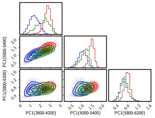
Projections of the first principal component, analogously to Fig. 4 in three different spectral windows, as labelled (the wavelength range is shown in Å). This figure illustrates the higher information content (understood as variance) in the bluer interval, that roughly maps the 4000 Å break. The contours engulf 25 per cent, 50 per cent, 75 per cent, and 90 per cent of each subsample.
We conclude in a more speculative tone: All the tests investigated in this study through PCA suggest that the structure of galaxies may be controlled by a single (or a few) parameters, as we can see through this result that only one component shows a correlation with age, and plays a main role as an evolutionary trend. Although the evolution of galaxies based on cold dark matter suggests that the properties of a galaxy should be controlled by a large range of physical parameters (Dalcanton, Spergel & Summers 1997; Mo, Mao & White 1998; Baugh 2006), our study is reminiscent of (Disney et al. 2008), who found that a single parameter could ‘explain’ most of the fundamental scaling trends of galaxies.
ACKNOWLEDGEMENTS
IF and ZS acknowledge support from the Spanish Research Agency of the Ministry of Science and Innovation (AEI-MICINN) under grant PID2019-104788GB-I00. OL acknowledges STFC Consolidated Grant ST/R000476/1 and a Visiting Fellowship at All Souls College, Oxford. Funding for SDSS-III has been provided by the Alfred P. Sloan Foundation, the Participating Institutions, the National Science Foundation, and the U.S. Department of Energy Office of Science. The SDSS-III web site is http://www.sdss3.org/.
DATA AVAILABILITY
This work has been fully based on publicly available data: galaxy spectra were retrieved from the SDSS DR16 archive (https://www.sdss.org/dr16/) and stellar population synthesis models can be obtained from the respective authors.
References
APPENDIX A: ASSESSING THE POTENTIAL EFFECT OF A SKY RESIDUAL
The study presented here is based on the science-ready spectra from the Legacy-SDSS survey. These data have been shown in many papers to be of the highest quality for detailed analyses of large samples, including work on stacked data (e.g. Gallazzi et al. 2005; Thomas et al. 2005; Rogers et al. 2007; La Barbera et al. 2013, 2014; Ferreras et al. 2019a). However, since PCA is overly sensitive to any potential systematic, in this appendix, we focus on the issue of sky subtraction, giving a quantitative upper bound on the contribution of sky residuals to the variance of the set. In Section 4, we argued that, due to the wide distribution of redshifts of our sample and the narrowness of the airglow lines, the net effect of residuals from sky subtraction are expected to be small, and not drive the signal in the highest principal components. We test this issue by taking a typical sky spectrum from the SDSS data base (see e.g. Hart 2019), producing sky spectra in the rest frame of the galaxies according to the redshift distribution of the sample. For simplicity, we restrict the analysis to quiescent galaxies, although the result is very similar for the other subsets. Fig. A1 compares the standard deviation of the sample – in red, identical to the red curves in the bottom panels of Fig. 1 – with that of the distribution of sky spectra (blue), noting that we also normalize the airglow spectra using the galaxy flux in the 6000–6500 Å for consistency. The left-hand (right-hand) panels correspond to the blue (red) spectral intervals explored in this work. The contribution from the sky is much lower, representing a fraction of the galaxy variance between 1/300 for the blue interval and 1/200 for the red interval. We emphasize that this comparison just shows the net maximum variance contributed by the sky spectrum to the analysis if it were not subtracted from the data. A typical residual in the sky-subtracted spectrum below the ∼5 per cent level will produce a contribution to the standard deviation ∼20 times smaller. To confirm this point, we note that the eigenvectors shown in Fig. 3 do not inherit the spectral structure from airglow, as one would expect if the sky were to contribute significantly to the analysis. In particular, this is more obvious in the red interval, where the airglow would introduce a large amount of variance in the redder part of the spectrum. While still in preparation, we also note that comparisons with synthetic spectra from hydrodynamical simulations of galaxy formation – that do not have any sky contamination added in the process, produce a distribution of spectra that is statistically very similar to the results presented here (Sharbaf et al., in preparation).
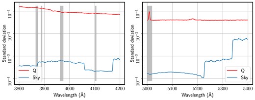
Comparison of the standard deviation in the quiescent galaxies (red lines) with that of the sky spectrum (blue lines) of the same galaxies, combined according to the redshift distribution, i.e. the sky spectra are brought to the rest-frame for each galaxy. The red lines are thus equivalent to those shown in the bottom panels of Fig. 1. The left-hand (right-hand) panels correspond to the blue (red) spectral intervals adopted in this work. Note this is an unrealistic worst case scenario, as it corresponds to spectra without any sky subtraction.
APPENDIX B: SPECTRAL FITTING FOR PCA IN THE RED INTERVAL
Concerning the result of the spectral fitting of stacked data according to extreme values of the principal component projections, we show in Fig. B1 the equivalent of Fig. 10 for the analysis performed in the red interval (5000–5400 Å), using the same fitting models and parameter ranges.
Equivalent of Fig. 10 when adopting the red interval (5000–5400 Å).
