


ABSTRACT
Measuring the size distribution of small (kilometre-scale) Kuiper belt objects (KBOs) can help constrain models of Solar system formation and planetary migration. Such small, distant bodies are hard to detect with current or planned telescopes, but can be identified as sub-second occultations of background stars. We present the analysis of data from the Weizmann Fast Astronomical Survey Telescope, consisting of fast photometry of ∼106 star-hours at a frame rate of 10–25 Hz. Our pipeline utilizes a matched-filter approach with a large template bank, including red-noise treatment, and injection of simulated events for estimating the detection efficiency. The KBO radius at which our survey is 10 per cent (50 per cent) efficient is 1.1 (2.0) km. The data from 2020–2021 observing seasons were analysed and no occultations were identified. We discuss a sample of sub-second false-positive events, both occultation-like and flare-like, which are still not fully understood but could be instructive for future surveys looking for short-duration events. We use our null-detection result to set limits on the kilometre-scale KBO number density. Our individual radius bin limits are consistent with most previous works, with N(r > 1 km) ⪅ 106 deg−2 (95 per cent confidence limit). Our integrated (all size) limits, assuming a power law normalized to large (≈45 km) KBOs give a power-law index q < 3.93 (95 per cent confidence limit). Finally, our results are in tension with a recently reported KBO detection from the ground, at the p = 4 × 10⁻⁴ level.
1 INTRODUCTION
Trans-Neptunian objects (TNOs) are a population of bodies found outside the orbit of Neptune. Some families of TNOs are thought to be remnants of the early stages of Solar system formation, and may be untouched by interactions with any of the planets (Dohnanyi 1969; Morbidelli, Brown & Levison 2003; Kenyon & Bromley 2004). As such, they could hold important clues to the formation history of our Solar system and to understanding the conditions present around young stars before their planets formed.
A subset of TNOs are Kuiper belt objects (KBOs), which reside in a belt at 30–50 au from the Sun, and clustered mostly a few degrees from the ecliptic plane. While hundreds of KBOs larger than a few kilometre have been identified, the smaller, but more abundant population remains hard to detect (Bernstein et al. 2004; Fuentes & Holman 2008; Fraser & Kavelaars 2009; Fuentes, George & Holman 2009; Schwamb et al. 2010; Petit et al. 2011).
Measuring the size and inclination distributions of kilometre-sized KBOs holds clues to the formation and evolution of the Solar system (Morbidelli et al. 2003; Kenyon & Bromley 2004; Schlichting, Fuentes & Trilling 2013), the origin of comets, (Duncan & Levison 1997; Levison & Duncan 1997; Volk & Malhotra 2008; Fraser et al. 2022), and the material strength of these bodies (Pan & Sari 2005).
Their small size and considerable distance from the Sun make them too faint to be imaged directly by current or planned telescopes. However, it is possible to detect kilometre-sized KBOs using serendipitous occultations of background stars (Bailey 1976; Roques, Moncuquet & Sicardy 1987), even though the rate of these occultations is very low. At any given moment, |$\mathcal {O}(10^{-9})$| stars are occulted by KBOs, and the duration of these occultations is typically a fraction of a second.
A search for such occultations in the Hubble Space Telescope Fine Guidance Sensor (HST FGS) yielded two detections of sub-kilometre KBO occulters (Schlichting et al. 2009, 2012), while searches for more occultations using ground-based telescopes is ongoing (Zhang et al. 2013; Arimatsu et al. 2017; Pass et al. 2018; Huang et al. 2021; Mazur et al. 2022). One detection from the ground has been published so far (Arimatsu et al. 2019), that could be evidence for an overabundance of KBOs larger than 1 km, generally consistent with findings from crater sizes on the surface of Pluto (Morbidelli et al. 2021). We note that even the two relatively secure detections in the HST FGS data have a false alarm probability of 2 per cent and 5 per cent, respectively.
In this work, we present the results of a dedicated survey for KBO occultations carried out using the Weizmann Fast Astronomical Survey Telescope (W-FAST; Nir et al. 2021b), during the years 2020–2021. A custom data reduction pipeline, described by Nir, Ofek & Zackay (2023) was developed to try to mitigate the different noise sources and false-positives inherent to ground base photometry, as well as inject simulated events into the extracted light curves to measure the expected efficiency of the pipeline. Even though our analysis includes ≈750 000 star-hours of usable data close to the ecliptic plane, the presence of correlated noise (e.g. from the atmosphere; see Osborn et al. 2015 and references therein) is shown to reduce efficiency for the detection of small occulters, consistent with detecting zero occultations in 2 yr’s worth of data, using published estimates for the density of small KBOs. We present seven occultation candidates detected by our pipeline that are most likely false-positives, for various reasons. The different sources of false-positives are discussed, and help demonstrate the difficulty of identifying true sub-second occultations in data from a single telescope.
With zero detections in our data set, we present upper limits on the number density of KBOs near the ecliptic plane, and compare them to previously published results. Per individual radius bin, our limits are similar to the results of Zhang et al. (2013) that have accumulated a similar number of star-hours but operated with three or four telescopes. We also combine the lack of detections in all size ranges to compare our null result with the models given by previous KBO detections. The power-law size distribution model given by HST FGS detections (Schlichting et al. 2012) is consistent with our result, while the recent detection from the ground (Arimatsu et al. 2019) is inconsistent with our null result at p = 4 × 10⁻⁴ confidence level.
We present the observatory and the data analysis in Section 2. We discuss the additional analysis performed on each of the occultation candidates in Section 3. We summarize the coverage provided by the 2020–2021 data set, as well as a summary of the candidate events, in Section 4. We set limits on kilometre-sized KBOs and discuss the challenges of detecting sub-kilometre KBOs from the ground in Section 5, and conclude in Section 6.
2 THE W-FAST OCCULTATION SURVEY
2.1 Data acquisition and analysis
W-FAST is a 55 cm, wide-field Schmidt telescope, equipped with a 7 deg2 field-of-view, fast-readout, low read-noise, sCMOS camera. The system was designed to explore the sub-second transient sky and to search for TNOs using the occultation technique (Bailey 1976). The observatory is currently located in Neot Smadar, Israel (see site description in Ofek et al. 2023). During the 2020–2021 observing runs, it had been located at Mizpe-Ramon, Israel.1 The W-FAST observatory is described in Nir et al. (2021b), while the KBO analysis pipeline is discussed by Nir et al. (2023).
Given the high data rate produced by the camera (about 6 Gbit s−1), we only saved cutouts around the 1000–5000 brightest stars in the field, rather than save full-frame images. The magnitude limit of stars depends on the exposure time and airmass, with stars of photometric signal to noise ratio (S/N) = 3σ having equivalent Gaia Bp magnitude of about 12–13.5. The spatial resolution, including atmospheric seeing and instrumental effects, moves between 5 and 10 arcsec, or 2 and 4.5 pixels with W-FAST’s 2.33 arcsec per pix scale. The cutouts were chosen to have a square side length of 15 pixels, to allow for the width of the point spread function (PSF) and also some room for mild tracking errors or vibrations of the telescope.
We applied a custom photometry pipeline to these small images (see details in Nir et al. 2021b, 2023). Dark and flat-field corrections were conducted on the individual cutout images. Photometry was measured using a centring procedure starting with a weighted aperture, which gives better results in finding the average centroid offset of the stars in their cutouts, which are then used to position an unweighted aperture on all stars. Some experimentation with PSF-weighted apertures was made, but the frame-to-frame flux measurements were less stable, presumably due to the time-varying PSF of images taken with short exposure times. In most cases apertures with a radius of 3 pixels were found to give the lowest noise. Background was measured on an annulus of 7.5–10 pixels, but was not subtracted from the flux measurements in order to reduce the total noise when looking for occultations. The background measurements were used to help disqualify bad events or entire segments of data, e.g. which were taken during morning twilight. Once light curves were produced, we searched them for occultations by applying a matched-filter (Turin 1960) with a template bank of 300–500 templates, spanning the parameter space of KBO occultations that we expect to be able to detect. Parameters include the impact parameter, occulter radius, star radius, time offset, and the transverse velocity between the star and the occulter (e.g. Nihei et al. 2007; Ofek & Nakar 2010). Since the light curves include substantial red noise (higher noise amplitude in lower frequencies) we applied ‘whitening’ to the filtering process (e.g. Venumadhav et al. 2019; Zackay et al. 2021).
Finally, in order to estimate the efficiency of our pipeline, we injected artificial occultations into the real light curves and applied our pipeline to the modified data as well. The resulting candidates are presented to a human scanner, without revealing any information that can bias his or her decision (e.g. the ecliptic latitude or the Earth’s projected velocity). This step is crucial in order to estimate the real efficiency of the search and cannot be replaced by analytical estimation. A more detailed description of the pipeline is discussed by Nir et al. (2023).
2.2 Observations
During 2020, the telescope had been operating nightly from about May through September, with a few additional nights in October–November. During 2021, it had been operating continuously from April to November, with a few additional usable nights in December. The observations discussed in this work span approximately 13 months of operations under generally good weather conditions. In total, the telescope had collected ≈840 h of usable, high-cadence data. The high-cadence observations discussed in this paper were obtained using either 10 or 25 Hz cadence. The 2020 data had all been taken at 25 Hz, with 30 ms exposure time (25 per cent dead-time). In 2021, following a software upgrade, the data were taken at 10 or 25 Hz, with negligible dead-time. The total number of star-hours observed was ≈1.75 × 10⁶, of which about 60 per cent was usable, for a total of ≈106 star-hours (the remaining 40 per cent was lost to various quality cuts, as explained by Nir et al. 2023). About 40 per cent of the observations were lost due to various quality cuts (see table 1 of Nir et al. 2023). The distribution of star-hours across ecliptic latitudes is shown in Fig. 1. The star-hours for all stars in a field are recorded as though the star’s ecliptic latitude is given by the coordinates of the centre of the field, not for the coordinates of each individual star. The bin widths in the plot are 2 deg and the field of view of the camera is ≈2.5 deg. The star-hours in this figure were divided into clusters at ecliptic latitude β < −11 deg, β > 22 deg, and −11 < β < 22 deg. The usable and total star-hours in each cluster are printed on the plot. In the central cluster, ≈95% of the star-hours are 4 deg away from the ecliptic plane. In each bin, the number of usable star-hours is about 60 per cent of the total star-hours. The observations taken off-ecliptic were used as a control group for the KBO detection methods. There is a ratio of ≈1:3 between the control and on-ecliptic observations.
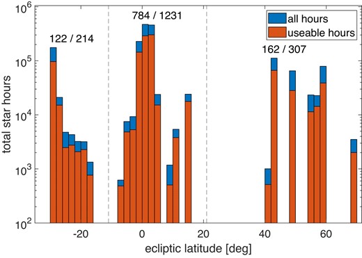
The number of star-hours in different ecliptic latitude bins. The ecliptic latitude for all stars in a given field is taken to be that of the centre of the field (with a width of ≈2.5 deg). The bins in this figure are 2 deg wide. The red bars show the number of usable hours that were not lost to various quality cuts. The blue bars represent the total star-hours observed. In most bars the fraction of good data is about 60 per cent of the total. We have clustered the observations into three sections: below ecliptic latitude β < −11 deg, above β > 21 deg, and close to the ecliptic plane at −11 < β < 21 deg. The number of usable and total star-hours is printed on the figure for each cluster (in thousands of hours). In the central cluster, 95 per cent of the star-hours are within ±4 deg of the ecliptic plane.
Since each star has different photometric properties, we also measured the distribution of star-hours across different photometric S/N values, which represents the noise in each individual measurement. The results are shown in the upper panel of Fig. 2. The histogram shows the distribution of star-hours for ecliptic and off-ecliptic fields. There is a correlation between the ecliptic fields and more numerous and fainter stars, since a large fraction of the star-hours were taken at the intersection of the ecliptic plane with the galactic plane. These fields contain more stars, and quickly accumulate star-hours. Apparently, there are more faint stars in these fields, which makes for lower S/N compared with the off-ecliptic fields.
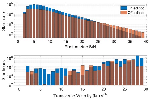
The number of (usable) star-hours as a function of photometric S/N (top panel) and transverse velocity (bottom panel). The blue columns represent the star-hours taken in fields close to the ecliptic, while the red columns are for fields away from the ecliptic. The ecliptic fields probably have lower S/N because they include many faint stars close to the Galactic Centre (which also coincides with the ecliptic) that contributed heavily to the total star-hours. The transverse velocity shows that the survey was biased towards high-velocity fields, with about 10 times more star-hours on fields with transverse velocities above 20 km s−1. The limiting magnitude, corresponding to S/N ≈ 5, is 13.5 for 10 Hz observations, and 12.5 for 25 Hz observations. While stars in that range are read-noise dominated, stars with magnibrighter than ≈9 are already dominated by scintillation and flat-field errors of 2–3 per cent, such that the photometric noise never improves beyond S/N ≈ 50.
Note that the S/N per measurement does not surpass ≈50, despite some small fraction of stars being considerably bright. It seems that at high frame-rates the relative shot-noise decreases as the photon count increases and at some point the error becomes a constant fraction of the flux, with a value of around 2 per cent. This irreducible photometric error could be due to atmospheric scintillations or differences in the gain of individual pixels that are not treated completely by the flat-field correction. Moving from 25 to 10 Hz did not dramatically decrease this noise floor, so we will assume at least part of the problem is due to flat-field errors. However, it should also be noted that some large changes in the star’s flux are sometimes seen, which appear to be atmospheric effects. We show some examples for such cases, where the pixel brightness changes visibly even on the same location on the sensor, when we discuss false-positives in Appendix B.
The observations also differ in their transverse velocity. This refers to the projection of the Earth’s velocity at the direction of the stars being observed. We assume all stars in the field have the same transverse velocity as the centre of the field at the time of observation. The total occultation velocity is the sum of Earth’s projected velocity and the specific occulter velocity, ≈4.7 km s−1 for circular, pro-grade orbits at 40 au. Since we do not know the specific KBO velocity a priori, and it is subdominant in most cases, we focus first on the Earth’s contribution to the overall velocity.
The transverse velocity has two effects on the expected KBO yield: (1) the rate of occultations grows linearly with the velocity, as more occulters traverse stars in a given time interval; (2) the occultations become wider at low velocities, making them easier to detect as there could be more images taken while the flux is affected by the occulter (see Ofek & Nir, in preparation). These are two contradictory factors, and we attempted to observe the ecliptic plane in a balanced range of velocities. Unfortunately, most of our observations are at high velocities, which has a big effect on the efficiency for detecting KBO occultations. The distribution of star-hours as a function of transverse velocity (taking into account only the Earth’s projected motion) is shown in the bottom panel of Fig. 2. There are roughly 10 times more star-hours at high velocities (20–30 km s−1) than at lower velocities. While this increases the expected number of occultations, it makes them hard to detect and discern them from data artifacts, as discussed in Section 5.3. In the future, we intend to dedicate more time observing the ecliptic plane fields far from opposition.
3 ANALYSIS METHODS
We analyse each candidate event that has passed our detection threshold and quality cuts (see Nir et al. 2023). Briefly, we applied a matched-filter approach (Turin 1960) using a template bank made by simulating occultation light curves, including diffraction effects and finite star sizes. We corrected for the effects of correlated noise on the power spectral density using the data itself to estimate the noise in different frequencies. We checked each light curve for instances where the flux is correlated between stars or correlated to other indicators such as instantaneous PSF width or star centroid positions, among other quality cuts, and used those to disqualify data that was affected by various systematics. Events that surpassed the detection threshold, i.e. time frames where the flux of any star, after being matched-filtered by any of the kernels, and normalized by the noise estimator, had a value higher than the threshold (nominally set to 7.5) were inspected by one of the authors, and more false-positives were ruled out. The remaining candidates are discussed in this work.
For each candidate we used the parameter estimation presented by Nir et al. (2023), and ran some additional tests that were added after the full analysis was done. These are used to validate (and rule out) occultation events for various reasons (e.g. atmospheric scintillations and detector artifacts). We discuss these tests in the following subsections.
3.1 Parameter estimation
For each of the events we perform Markov Chain Monte Carlo (MCMC) sampling to get an estimate of the distribution of occultation parameters posteriors, given the light curve of each event. We follow the same analysis presented by Nir et al. (2023) with the following modifications: (1) We fit the time offset between the middle of the light curve and the middle of the occultation template, allowing for some offset between the two, even though we begin the analysis by centring the light curve on the peak of the event (the point where the matched-filter result is maximal); (2) we set a non-uniform prior on the velocity (see equation 4 and Fig. 3); (3) we run 20 000 points in each chain, throwing away (‘burning’) half of each chain; and (4) we use 50 chains with random starting positions, and use an additional rule to reject entire chains.
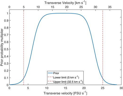
The prior used to limit the velocity parameter v given by equation (4). The exponential edges provide a soft stop for the MCMC sampler, without biasing the results for velocities in the middle of the range.
Nir et al. (2023) had rejected chains where the χ2 per degree of freedom was substantially larger than the median of all chains (three times the median absolute deviation of all chains). We adopt this but first disqualify chains where most of the templates are so shallow they are essentially undetectable. To quantify this rule, we measure the median signal of the templates in the chain. We define the signal of a specific template as
where fi is the template flux in frame i (normalized such that the flux outside the occultation is 1), 〈f〉 is the mean flux of the template, and σphot is the measured noise of the actual event. S is an estimate of the S/N that would be measured for such an occultation, triggering by exactly the same template (an ideal matched-filter). We rule out any chain with a median S < 3.5, which is much lower than our actual detection threshold of 7.5. The decision to rule out chains based on the different values of χ2 is made using only chains that survived the signal rule.
The goal of the priors used for the five parameters of the fit is to limit the parameters to reasonable values that can arise from real occultations, and reflect our previous knowledge of the event characteristics. We attempted not to bias the results and use either flat or nearly flat priors where possible. For example, we chose to leave a uniform prior on the occulter radius r, despite knowing that the size distribution is generally fast dropping with occulter radius. The range of allowed values is 0.1 ≤ r ≤ 3 FSU (which is the typical size scale for diffractive occultations given by |$\sqrt{\lambda D /2}=1.3$| km for our observations, using the observed wavelength λ = 550 nm and the estimated distance to the Kuiper belt of D = 40 au).
The impact parameter, b, and the time offset, t, are both nuisance parameters and have no physical reasons to be close to any value. We used a flat prior on b, but because we are first centring the light curve to fit the template, we assumed the time offset should be small, and applied a Gaussian prior,
where σt = 100 ms. Note that the priors are not normalized because the Metropolis–Hastings algorithm only ever uses the probability ratios between points so the normalization of the priors generally cancels out. The prior on the stellar size, R, is also given as a Gaussian, reflecting our belief in the successful fit of the star’s temperature based on the measured Gaia colours:
where R0 is the fit result and σR = R0/10, all in Fresnel units. The colours are based on cross-matching the star’s position with the Gaia data release 2 (DR2; Gaia Collaboration 2018). We used a velocity prior that was not used by Nir et al. (2023). The shape of the prior is set to a two-sided exponential function with a flat plateau in the middle:
where vℓ = 3.8 FSU s−1 (≈5 km s−1) and vh = 25 FSU s−1 (≈32.5 km s−1) are the edges of the range of likely values of transverse velocities of the Earth-KBO system, and P0 = 0.1 is a constant that tunes the size of the flat region in between the edges. A plot of the velocity prior values is shown in Fig. 3. This prior allows for limiting the sampler from going into unphysical values without placing a hard stop on the chains, but at the same time does not heavily bias the resulting values towards high or low velocities inside the allowed range.
Finally, we are mostly interested in the posterior results for the physical parameters of the occultation, r and v, so we present the posteriors after marginalizing over the remaining t, b, and R. For the single parameter marginal posteriors we find the shortest interval containing 68 per cent of the distribution and use that as confidence intervals, as discussed in Nir et al. (2023). We use the parameter estimates to check if the light curve is consistent with the transverse velocity of the Earth, for the field in which the event was detected. For example, the MCMC analysis results for the first candidate event are shown in Fig. A2.
3.2 Nearest neighbour analysis
During regular analysis we disqualify events that occur at a time when other stars in the field show similar features to the occultation candidate (see Nir et al. 2023). For the short list of candidates we have left we also check if nearby stars show flux variability at slightly earlier or later times. This may happen if any atmospheric event passes across multiple stars but not exactly at the same time (e.g. a cloud or focusing/defocusing bubble of air).
The typical angular distance between bright stars in our field is 1–6 arcmin. Assuming the typical velocity is 15 arcsec s−1, it is also reasonable that stars separated by ∼3 arcmin will be affected by a localized atmospheric event within a time interval of ∼10 s. This is the time-scale of a double batch of 200 frames (8 or 20 s, depending on the cadence).
We choose the closest stars to the occulted star, that have a photometric S/N > 5, and plot the flux for that batch of 200 frames when the candidate event occurred. This qualitative method gives us another chance to find localized atmospheric events that would otherwise not trigger our data quality cuts because they do not occur simultaneously on different stars. We show the nearest neighbour analysis for one of the likely atmospheric events in Fig. A4.
3.3 Outlier analysis
Another possible false-positive could be caused by instrumental effects (sensor defects, telescope reflections, etc.). To check if a candidate event’s flux is stable over longer periods outside the 200 frames where it was detected, we loaded the long-term flux values for all stars in a region of 2000 frame before and after the event. This translates to 80 or 200 s of data in either direction, for 25 or 10 Hz cadences, respectively.
For each star we subtract a smoothed flux, that we get using a Savitzky–Golay filter with a 3rd order polynomial and a 101 frame window size. The values of this mean-subtracted flux are iteratively fit to a Gaussian distribution, while removing any outliers of more than three times the noise RMS. We count the number of outliers removed by this sigma clipping procedure and check if the target star has an unusually large number of outliers (>50) compared with other stars during that time period (typically 20–30 outliers in the time range we check).
Stars with many outliers can be disqualified as having unstable flux over time (e.g. due to a nearby bad pixel). We also display the distribution of stars with many outliers on the image plane, to see if any clustering of unstable stars is evident on the camera’s sensor. An example for such an outlier analysis is shown for one of the likely atmospheric events in Fig. A3.
3.4 A note about main-belt and near-Earth occulters
Some care should be taken when deducing the physical parameters of an occulting object based on the estimated parameters of an occultation. Throughout this work we assume the occulter is in the Kuiper belt, with a nominal distance of 40 au. This simplifies the parameter estimation process but a more careful analysis should be done on any real occultations, including allowing the distance (and thus, the Fresnel scale) to vary as well.
A considerably smaller distance could occur when considering other occulter populations. An occultation caused by a main belt asteroid could resemble a KBO occultation in terms of the width and depth of the event. Taking as an example an object with a circular orbit with a radius of 2.5 au, the Fresnel scale would be ≈250 m (as seen from Earth, at opposition). The relative velocity of such objects would be about 44 FSU s−1, which can be confused with high-velocity events in fields with high transverse velocity. However, the number of main belt asteroids is estimated to be about 107 objects above 250 m (Davis et al. 2002; Maeda et al. 2021). Spread out over thousands of square degrees of the main belt, the estimated density would be 103–104 objects per degree squared. So the number density per square degree of main belt occulters is at least an order of magnitude smaller than the estimate of ≈105 km-scale KBOs per square degree given by Schlichting et al. (2012).
Near Earth objects would have an even smaller Fresnel scale, and thus, in most cases, occultations that are substantially shorter than the W-FAST exposure time. Their population is also considerably smaller and the chance for occultations is expected to be lower than that of the main belt population.
4 RESULTS
We present the results of the analysis pipeline over the data collected in 2020–2021. We summarize the status of a few occultation-like false-positives which are ruled out for various reasons. We then discuss the efficiency for detecting occulters of various sizes and estimate the expected number of detections based on existing size distribution power-law models.
4.1 Occultation candidates
Our search resulted in eight occultation candidates passing both the quality cuts and the human inspection, as described in Nir et al. (2023). All these events were eventually rejected based on deeper inspection of the data.
One of these events, upon second inspection, was shown to be close to a warm pixel, which produced slightly higher values but was not flagged by the data pipeline. We summarize the properties of all remaining seven candidates in Table 1, where it is clear that none of the candidates is fully consistent with what we expect from a KBO occultation. Some are clearly false-positives, such as events with many outliers in the long-term light curves (this includes the events of 2021 April 11, 2021 April 12, and 2021 April 16). Note that the candidates’ star in these cases is subject to an unusually high number of flux outliers. Most other stars in the same data set do not show many outliers (more than 90 per cent of the stars, as seen in the top panels of the relevant figures, e.g. Fig. A12). Thus we are confident that the flux outliers are the cause of these candidates, and not merely background phenomena that coincidentally accompanied these events.
Summary of candidate occultations. The ecliptic latitude (β) is given for the centre of the field of view of the observations. The event S/N is the integrated matched-filter result for the entire event, while the photometric S/N is the single-frame flux versus noise measured over the previous 2000 frames. The stellar size (R⋆) is given in Fresnel Scale Units (FSUs), and was calculated using a fit to Gaia DR2 colours. The FWHM (full width at half-maximum) is given in arcsec, where the combined atmospheric and instrumental seeing is commonly in the 4.5–5.0 arcsec range. The airmass and transverse Earth velocity (VEarth) are calculated for the centre of the field at the time of the event. The parameter ranges for occulter radius r and occultation velocity v are from the MCMC fit (see Section 3.1). In cases where the posterior is bi-modal we show two options for the ranges as (i) and (ii). Events that are marked as having ‘Neigh. stars’ are those where there is some variability detected by eye in the light curves of the neighbouring stars. Events that are marked as ‘Flare-like’ display strong flux increase in addition to dimming. The number of outliers is calculated in the 4000 frames around the event time, where most stars will produce 20–30 outliers just due to statistical fluctuations.
| Event time (UTC) | Coordinates | β | Event | MG | Teff | R⋆ | Phot. | f | FWHM | air | VEarth | r range | v range | Neigh. | Flare- | Num. |
|---|---|---|---|---|---|---|---|---|---|---|---|---|---|---|---|---|
| (deg) | S/N | (○K) | (FSU) | S/N | (Hz) | (arcsec) | mass | (km s−1) | (km) | (km s−1) | stars | like | outliers | |||
| 2020-07-01 20:58:01 | 19:32:42.6+21:25:23.4 | 42.8 | 7.63 | 9.72 | 5342 | 1.1 | 22.41 | 25 | 5.34 | 1.09 | 27.2 | 1.9–3.4 | (i) 8–10 (ii) 13–28 | No | Yes | 25 |
| 2021-04-01 17:29:08 | 06:31:34.0+20:33:54.8 | −1.7 | 7.54 | 11.41 | 6640 | 0.4 | 18.64 | 10 | 5.65 | 1.13 | 4.0 | 0.5–1.5 | 19–28 | Yes | No | 21 |
| 2021-04-03 17:00:36 | 06:31:57.7+20:21:56.8 | −1.7 | 8.42 | 11.89 | 6464 | 0.5 | 19.24 | 10 | 5.18 | 1.09 | 5.0 | 1.4–3.3 | 22–29 | No | No | 19 |
| 2021-04-11 18:36:45 | 10:20:42.6+09:00:32.8 | −1.7 | 7.65 | 12.92 | 6488 | 0.3 | 10.64 | 10 | 4.84 | 1.08 | 9.5 | 0.6–0.9 | 15–21 | Yes | No | 79 |
| 2021-04-12 20:22:19 | 10:22:38.2+07:27:50.7 | −1.7 | 7.54 | 12.80 | 5388 | 0.4 | 8.49 | 10 | 5.26 | 1.19 | 9.3 | (i) 1.0–2.5 (ii) 0.6–1.0 | (i) 17–30 (ii) 6–8.5 | Yes | No | 62 |
| 2021-04-16 20:45:56 | 13:32:52.1-09:48:57.8 | 0.0 | 8.07 | 11.94 | 5886 | 0.4 | 8.31 | 25 | 4.58 | 1.37 | 21.2 | 0.6–2.1 | 17–25 | Yes | No | 119 |
| 2021-09-14 17:58:01 | 22:00:23.2-11:34:15.3 | 1.3 | 7.53 | 11.84 | 5961 | 0.6 | 11.53 | 10 | 7.00 | 1.61 | 20.3 | 0.55–0.9 | 7–8.5 | No | Yes | 21 |
Other candidates seem likely to be atmospheric, such as the events of 2020 July 1 or 2021 September 14 that show both a decrease and an increase of flux, appearing ‘flare-like’, which makes them suspiciously similar to a sample of 30 flare events, with sub-second time-scales, that are most likely to be non-astrophysical, but a mixture of atmospheric events and satellite glints (Nir et al. 2021a). These flares are discussed further in Appendix B.
A single event was detected in an off-ecliptic field (the event at 2020 July 1) making it unlikely to be a KBO occultation. It is also the only event detected in the 2020 data. The remaining six events were taken in 2021 on ecliptic fields. Five of the events occurred in the first half of 2021 April, raising further suspicion that they are not real occultations. Note that the flare events were found in both the 2020 and 2021 data sets.
Two events are single-frame events where there is insufficient information to confirm or rule out the events, but the low frame rate and low projected Earth velocity make them unlikely to be KBO occultations. For several events, there is some level of inconsistency between the field’s projected Earth velocity and the best-fitting velocity of the putative occultation. Simply put, the dip in the light curve was either too narrow or too wide for the expected event duration. The expected Earth’s projected velocity can be compared with the MCMC fit to each event in Table 1. Note that the Earth’s projected velocity does not include the unknown occulter velocity (for a pro-grade, circular orbit at 40 au, the occultation velocity will be smaller than the Earth’s projected velocity by ≈4.7 km s−1). Because we see several events that are inconsistent with the Earth’s projected velocity, we cannot assume that the events that are consistent are true occultations, as they can, just as likely, be artifacts that just happened to occur on a field with the ‘correct’ projected velocity. In any case, in Table 1 we show that even the events with a consistent velocity are ruled out by other tests, such as the number of outliers or variability in nearby stars’ flux.
We discuss each occultation event separately in Appendix A, and rule out each of them as being a true occultation. In Appendix B we discuss a sample of short-duration flux-increases (‘flares’). Assuming some of the flares in that sample are atmospheric, further strengthens the hypothesis that some of our occultation candidates are also caused by atmospheric events.
4.2 Efficiency for detecting occultations
A rough estimate of the number of expected detections for each star can be calculated using the average transverse velocity, the maximum impact parameter, and the surface density of occulters. The transverse velocity can be taken to be roughly 20 km s−1. The impact parameter is the angular distance at closest approach between the centre of a star and the centre of an occulter. We can estimate the maximum impact parameter at which the event is still detectable to be about a Fresnel-scale, ≈1 km (projected at the distance of the occulter). Thus each star subtends a strip of width 2 km and length 20 km every second. At a distance of 40 au, this covers an angular size of ≈1.3 × 10⁻¹¹ deg2 every hour.
The measured angular density of KBOs, given by Schlichting et al. (2012), is N(r > 250 m) = 1.1 × 10⁷ deg−2, with a differential power-law index q = −3.8, so the cumulative distribution is N(>r) ∝ r−2.8. If we assume we can detect occulters with a radius of 0.5 km, the number density becomes ≈1.6 × 10⁶ deg−2. Thus, we will require ≈50 000 star-hours to detect a single occultation. If we can only detect occulters of radius 1.5 km or larger, the surface density becomes 7.3 × 10⁴ deg−2, and the number of star-hours per detection becomes ≈106. Using these rough estimates, it seems that with 750 000 star-hours the survey presented in this work should be able to detect a few occultations with an occulter radius of ∼1 km.
A more careful analysis needs to also take into account the efficiency for detecting occulters of different radii. During the analysis, we have systematically injected simulated occultations with different parameters into the raw light curves, and tested what fraction of the events were detected. Using ≈105 simulated events we calculate the detection efficiency at each occulter radius (with bins of size 0.1 km). See Nir et al. (2023) for more details on these simulations. The results are shown in Fig. 4. The black line represents the average efficiency for that occulter radius bin, with grey areas representing the Poisson (statistical) uncertainties associated with the number of detected events. The detected and total number of simulated events in each bin are shown as red numbers above the line.
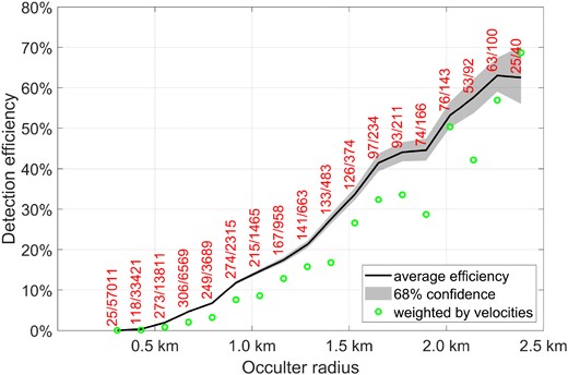
The detection efficiency for occulters of various sizes over the data collected during the 2020–2021 observing seasons. The black line represents the overall efficiency, assuming a uniform distribution of transverse velocities of observations. The grey areas represent the uncertainty due to Poisson (counting) errors. The red numbers show the number of simulated, injected events in each size category (detected and total number of events). The events were generated using a flat distribution of velocity and impact parameter. The stellar S/N and angular size were taken from the actual star’s light curve and Gaia data, respectively. The occulter radius was drawn from a steep power-law distribution. The distribution of impact parameters for real occultations is expected to be uniform, but the distribution of velocities in our observations is weighted towards higher velocities (see Fig. 2). A weighted average efficiency is shown as green circles, showing that the real efficiency in our data set is lower than suggested by the raw detection fractions across all events. In any case, it is evident that the detection rate at small radii (<1 km) is only a few percent at best.
Each simulated event has parameters drawn from random distributions. The transverse velocity and impact parameter are chosen from a uniform distribution, while the radius of the occulter is chosen from a steep power law that is both more realistic and helps generate enough detections even at the smaller sizes where events are hard to detect. The photometric S/N is taken directly from the light curve, and the stellar angular size is calculated using the star’s cross-match to the Gaia DR2 data base (Gaia Collaboration 2018). Since stars are chosen randomly from the stars tracked in each field, the distributions of stellar size and S/N are representative of the sample as a whole. The uniform velocity distribution is not a good representation of our data, since most of the data has been collected at high transverse velocity (>20 km s−1). Using the distribution of star-hours in different velocity bins, we re-weigh the efficiency to calculate more realistic (and lower) efficiency values and show them as green circles on the plot.
The efficiency for detecting small occulters, with radius <1 km, is only a few percent, either when averaging the detections of all velocities, or when re-weighing based on the time spent in each velocity. It is thus more obvious why the simple estimates made at the beginning of this section are highly optimistic. In fact, such low efficiency means more than an order of magnitude more star-hours are required to make a single detection.
We also note that the injected events are only put into regions of the light curve where there are no quality flags or other event candidates. So, the efficiency fraction does not include the fraction of time that is flagged as ‘bad data’. This is accounted for when calculating the coverage by only including the ‘good data’ when estimating the total coverage and number of detections. Furthermore, each simulated event has been vetted by a human ‘scanner’, which also may reduce the number of detected events. We noticed that more than 90 per cent of simulated events that had triggered were also correctly identified by the vetting process, so we ignore the contribution of the human in estimating the efficiency.
To estimate the total number of expected occultations, we calculate the efficiency separately for each value of the relevant parameters, and multiply that by the number of star-hours in that parameter bin. The coverage is the number of square degrees that were monitored, in which some occulter radius range would have been detected, weighed by the efficiency relevant for that selection of stars, transverse velocity and impact parameters:
where v(t) is the projected velocity in each observation, ε is the detection efficiency for each occulter radius r (calculated from injection simulations), and bmax = 2 FSU is the maximum impact parameter where we injected simulated events (most events with b > bmax will not be detectable). The integral over b is simply 2bmax, and the integral over time is simply done by summing the star-hours at different velocities. For the coverage presented in this work we used only star-hours collected at a distance of ±5 deg from the ecliptic plane, and assume the density of KBOs in that region is uniform.
To compare the coverage to the expected number density of occulters, we plot the inverse of the coverage in Fig. 5. Counting only observations close to the ecliptic, we get a total of ≈740 000 star-hours. The blue crosses represent the inverse coverage, with horizontal errors spanning the radius interval of each bin, and the vertical errors representing the statistical uncertainty derived from the efficiency calculation, which themselves come from the counting statistics of injected detections. The black line and grey area represents the KBO model given by Schlichting et al. (2012), including the uncertainties of both the overall number of objects and the power-law index. The numbers above each radius bin represent the expected number of detections for that bin alone, with uncertainties calculated as the quadratic sum of statistical uncertainties from the efficiency and the KBO number density. It is evident that, using the KBO density model, we expect to get less than one event in each bin. At low radii, there are many more occulters, but the low efficiency reduces the coverage dramatically, as evident from the rise of the blue crosses on the left. For higher radii, the efficiency approaches 100 per cent but the number of occulters is expected to drop quickly. The most sensitive part of the radius distribution is around 1 km, but not by a large factor. The total number of expected detections, including KBOs of all sizes in this range, is |$1.8_{-1.6}^{+3.8}$| events. The combined uncertainties of both the efficiency and the density model, make this number consistent with either five events on the optimistic side, and with zero events on the pessimistic side (with 68 per cent confidence intervals). If events were detected, they are not substantially more likely to be detected with a certain occulter radius, but with a slightly higher probability to be in the range of 0.5 < r < 1.5 km. It is also evident that if the number density had a dramatic increase above 1 km, e.g. a break to a shallower power law that increases by a factor of a few the number of occulters in the 1 < r < 2 km range, it would be improbable that we would not find any occultations in our data.
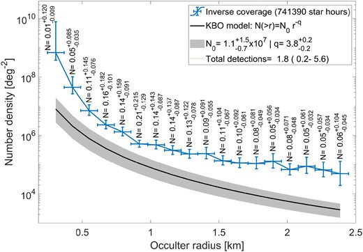
Inverse coverage as a function of occulter radius, compared with the expected KBO number density (per radius bin of size 0.12 km). The blue crosses represent the inverse number of deg2 covered by the current data set, including the efficiency for detection, at each given occulter radius bin, considering the star-hours taken at different observational parameters. The horizontal errors simply span the width of each size bin, while the vertical errors include the statistical errors due to the counting (Poisson) errors on the number of detected simulated events that were used to estimate the efficiency in each bin. The black line and grey area represent the best model for the number density of KBOs close to the ecliptic given by Schlichting et al. (2012), along with the uncertainties on the total number and the power-law index. The numbers above the crosses are the expected number of detections in each size bin, including errors from both the efficiency and the KBO density model. The total number of expected detections integrated over all sizes in this plot is |$1.8_{-1.6}^{+3.8}$|.
Finally, we show that after treating the light curves for red noise, removing segments of bad data, and setting a high threshold for detection required to reduce the number of false-positives, we are left with a low efficiency, that can dramatically increase the number of star-hours required for even a handful of detections. The naive expectation that a few tens of thousands of star-hours are sufficient to detect a KBO occultation underestimates the difficulty of this kind of search from the ground, especially using a single telescope.2 With more than a million star-hours we are still left without a single confirmed detection. We discuss the implication of our results in Section 6.
5 DISCUSSION
5.1 Limits on the kilometre-scale KBO number density
Assuming none of the candidates in our sample is a real KBO occultation, we can place upper limits on the underlying density, using the efficiency calculated from the fraction of detected simulated events. The model we have used in Fig. 5, adapted from the results of Schlichting et al. (2012), already represents a good upper limit estimate, as the integrated number of events we expect from that model and our efficiency estimate is |$1.8_{-1.6}^{+3.8}$| events. This is still consistent with zero detections, but a model with substantially larger density, particularly at r > 1 km, would already be in tension with our findings.
A more quantitative calculation allows us to draw a contour of the 95 per cent confidence upper bound, based on the coverage in each occulter size bin. The coverage calculated in equation (5), shown in Fig. 5, can be used to calculate the expected number of KBO occultations in either each radius bin, or integrated over all sizes where our survey is sensitive:
where the differential number of KBOs per solid angle is given by n(r) ∝ r−q. We probe the range 0.25 < r < 2.5 km, which is the range that we used in the injection simulations, and also contains most of the detection potential. The individual estimated number of detections for each radius bin is shown above each point in Fig. 5, assuming the model from Schlichting et al. (2012).
The lack of detections allows us to calculate the upper limits in various scenarios. In the following calculations, we calculate 95 per cent upper limits by setting Nexpected = 3, which is the Poisson expectation value that gives a 5 per cent probability to measure zero occultations.
One way to set the upper limits is to calculate the number density limit individually for each bin. This result is plotted as the solid, blue line in Fig. 6. The limits are fairly consistent with the results of TAOS (Zhang et al. 2013), that also had accumulated ≈106 star-hours over 7 yr.
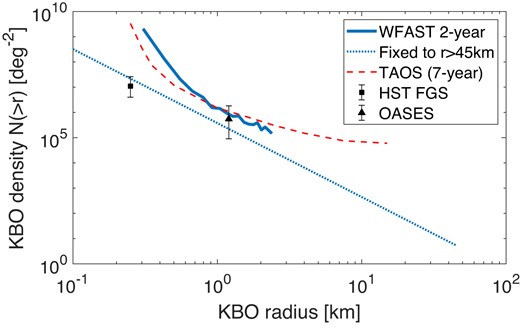
Measurements and upper limits on the number density of KBOs that are larger than some radius, N(>r), for various occultation surveys. The solid, blue line is the upper limit by this work, calculated individually for each radius bin. The dashed red line is a similar upper limit given by TAOS I (Zhang et al. 2013), which is fairly consistent with our results, including a similar number of star-hours but with three or four telescopes. The black square is the measurement given by Schlichting et al. (2012), using the HST fine guidance sensor. The black triangle is the measurement given by Arimatsu et al. (2019), using OASES (a ground based observatory with two telescopes). The dashed, blue line is the steepest power-law model that is normalized to the measured number density of KBOs at r = 45 km, that is also consistent with our null detection over all radius bins.
The dashed, blue line in Fig. 6 shows the upper limit on a power-law model for KBOs which is normalized to the number density at 45 km, given by Fuentes et al. (2009), with a power-law index q < 3.93. Any steeper (more negative value) power law would generate an expected number of detections above 3, and would be ruled out at a 95 per cent confidence level by combining the lack of detection on all size bins.
5.2 Comparison to previous results
Previous detections of KBOs from the HST FGS include two occultation events, and a third candidate at high ecliptic latitude which is deemed to be a false-positive (Schlichting et al. 2009, 2012). From those measurements, and the number density calculated for large KBOs (>45 km) they propose a power-law model for smaller KBOs, with a single power-law index of q = 3.8 ± 0.2. This result, shown as a black square in Fig. 6, is consistent with the power-law index limit from our survey (q = 3.93, dotted, blue line). We can check the parameter space of models that are defined by N(>250 m) and q, with values close to those of the model given by Schlichting et al. (2012). For each pair of parameter values we calculate Nexpected, considering the coverage we have over all occulter size bins. The results are shown in Fig. 7.
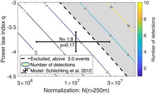
The parameter space of power-law models for KBOs, for models similar to the result of Schlichting et al. (2012). The contours show the expected number of detections, given our coverage, for a pair of model parameters defined by the normalization at 250 m and the power-law index. The shaded region is excluded at the 95 per cent confidence level. The fiducial value and uncertainties given by Schlichting et al. (2012) are shown as black error bars. The values printed next to the fiducial value show the expected number of detections in our survey (N = 1.8), and the Poisson probability to measure zero detections given the stated expectation value (p = 0.17). This model is in some tension with our results, but is not ruled out with more than 83 per cent confidence.
The most recent detection of a small KBO occultation comes from a ground survey, using a system of two telescopes with only a small sample of a few 104 star-hours (Arimatsu et al. 2019). This detection, if real, indicates an uptake in the size distribution at a radius of 1–2 km. This result is consistent with theoretical models, e.g. Schlichting et al. (2013). Morbidelli et al. (2021) also indicated an increase in the number of KBOs, based on analysis of the crater size distribution on Pluto. It is somewhat surprising, that with an order of magnitude more star-hours, no such occultations were seen in our survey. The power-law upper limit model shown as a dashed, blue line in Fig. 6 is already below the results from Arimatsu et al. (2019). To quantify this, we test models similar to the parameters presented by Arimatsu et al. (2019) and check which values are consistent with our null detection across all radius bins. The results are shown in Fig. 8. Their density model would yield Nexpected = 7.8, which is inconsistent with our null detection at the p = 4 × 10⁻⁴ level.
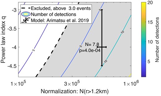
The parameter space of power-law models for KBOs, for models similar to the result of Arimatsu et al. (2019). The contours show the expected number of detections, given our coverage, for a pair of model parameters defined by the normalization at 1.2 km and the power-law index. The shaded region is excluded at the 95 per cent confidence level. The fiducial value and uncertainties given by Arimatsu et al. (2019) are shown as black error bars. The values printed next to the fiducial value show the expected number of detections in our survey (N = 7.8), and the Poisson probability to measure zero detections given the stated expectation value (p = 4 × 10⁻⁴). Thus, the measured abundance reported by Arimatsu et al. (2019) is inconsistent with our results.
There are some possible explanations for this tension:
The sensitivity of the two telescopes used by Arimatsu et al. (2019) is substantially higher, due to the lower detection threshold allowed by cross-matching the light curves of the two telescopes. The signal-to-noise ratio of each individual detection they present is ≈5, compared with the threshold of 7.5 used in our survey. However, their estimate of the occulter size is 1.3 km, which is large enough to be detected by our pipeline in at least 15 per cent of the parameter space (see Section 4.2). While the sensitivity may affect the number of star-hours required to make a detection, the KBO density reported in previous works already takes the into account the sensitivity of those surveys. The density reported in Arimatsu et al. (2019) is inconsistent with our estimates, regardless of the number of star-hours, the number of telescopes, and the efficiency of that survey. Furthermore, the fact that the TAOS I survey (Zhang et al. 2013) found no occultations, even with three or four telescopes and ≈106 star-hours, makes this explanation insufficient.
The detection reported by Arimatsu et al. (2019) is actually an unlucky coincidence of two atmospheric artifacts at the same time. This is also unlikely, since the two light curves appear consistent in shape and timing. On the other hand, even looking just at the two seconds before and after the candidate event, the OASES-01 light curve (their Fig. 2, blue line) shows at least one instance where the flux increases in amplitude similarly to the dip that is part of the occultation event. If even one telescope is frequently subject to random correlated fluctuations of similar amplitude to the one constituting the occultation candidate (such as those presented in Appendix B), it becomes considerably more likely that the event they reported is caused by coincident fluctuations and not an occultation.
This single detection is a ‘lucky accident’ with a probability of 4 × 10⁻⁴.
The analysis presented in the methods section of Arimatsu et al. (2019) shows that there is no overabundance of fluctuations outside the occultation candidate event, in the 20 min surrounding it, and no large atmospheric events coincident with it affecting other stars. Even so, in some of the event candidates discussed in Section 4.1 there is no evidence for a large number of outliers or any flux changes in nearby stars. A dedicated search for false-positives over a larger part of their data, inspecting localized fluctuations, is required to gain more insight into the nature of this event. Further detections (or lack thereof) of new occultations in data collected after this event was identified in 2016, would also help shed light on the subject.
It is interesting to note that even the baseline model of KBO density we used here is not beyond suspicion. Those results, based on two detections from space, reported in Schlichting et al. (2009, 2012), would not be subject to the false-positive events caused by atmospheric fluctuations. Based on their own bootstrap simulations, Schlichting et al. (2012) estimate the false alarm rate for their event to be 5 per cent. Schlichting et al. (2012) also report a false detection on an off-ecliptic field. While they rule out that event because of its incompatible ecliptic latitude, the fact such false-positives exist brings into question the validity of the on-ecliptic detection. The two events are not very different in the shape of their light curves, and it is not clear why one should be more believable than the other, besides the position on the sky of the occulted star. If even images taken from space can be affected by such spurious detections, it is not surprising if later, ground-based surveys are hard-pressed to identify real occultations from various false-positives.
Some of the uncertainty surrounding these past detections could be cleared up once additional surveys, e.g. OASES, TAOS II, and Colibri (Arimatsu et al. 2017; Huang et al. 2021; Mazur et al. 2022), would publish their results. Characterization of various systematics such as discussed in this work, especially from surveys with multiple telescopes, could help explain the plausibility that such artifacts could appear in two telescopes at the same time.
5.3 False detections
When looking for short duration, rare events with only a single telescope, care must be taken to avoid rare occurrences of different types of foregrounds. It is particularly difficult to know if an event is real without confirmation from another observatory, preferably one located a few tens of meters away such that it observes through different instances of the atmosphere. Even with two telescopes, relatively common foreground events (such as scintillation or wind-driven tracking errors) can occur in both images simultaneously when large amounts of data are accumulated. In this work, we have applied multiple layers of foreground rejection methods (automated quality cuts, human vetting, and additional ad hoc tests for found detections discussed in Section 3).
Clearly there are some hard-to-reduce foreground events to consider when searching for occultations by sub-kilometre KBOs. The candidates presented in this work, though surpassing the detection threshold and not triggering any of the data quality cuts we applied, are all most likely to be instrumental or atmospheric artifacts. Some show many outliers, some have suspicious variations in the flux of nearby stars, and most of them do not show the expected width compared with the Earth’s projected velocity. Five out of seven events occurred in the first half of 2021 April, further hinting that the source of those events is instrumental or environmental. In addition, we detected 30 flare events (see Appendix B), of which some also show dimming besides the brightening, making it clear that false detections are much more common than real detections, and indistinguishable from them.
The large number of false detections we see in our data also suggests that if not carefully controlled, such events could also occur coincidentally in two telescopes, particularly under bad atmospheric conditions. One hint for such bad conditions comes from the clustering of candidates in 2021 April, where five out of seven events are detected.
A survey with two telescope might set a lower threshold that allows for a higher false alarm fraction. A single telescope observing 106 star-hours at 25 Hz would need a false-alarm rate of ≈10−11 to get one false detection in the entire survey. A naive approach to adding another telescope would be to increase the single-telescope false-alarm rate by a factor of 1011 (e.g. by dropping the threshold from 7.5σ to 3σ). If atmospheric events such as presented in this work are instead concentrated in a 2 week period (instead of uniformly across 2 yr) then the coincidence rate of would be 50 times higher. If atmospheric instability has shorter typical durations, it may be that for short periods of times, two-telescope events become even more likely.
If the distribution of foreground events is much flatter than a normal distribution (i.e. events are in the ‘long tails’ of the distribution), the rate could be less affected by the decrease of threshold. It should be noted, however, that five out of seven events have a total score (matched-filter S/N) of 7.5–7.7, indicating that the distribution is not completely flat. This suggests that before setting a threshold for an experiment with more than one telescope, a study of the distribution of low-threshold events, as a function of time and S/N, should be made on each telescope, to make sure the combined false-alarm rate is well controlled.
6 CONCLUSIONS
We presented the results of a dedicated occultation survey for kilometre-scale KBOs using the W-FAST observatory, over the 2 yr period of 2020–2021. Using a single telescope, we collected ≈740 000 star-hours on low ecliptic latitudes, and combined with data quality cuts, human vetting and injected simulations, we establish a competitive upper limit on KBOs in the size range of 0.5–2.5 km.
We detect seven possible occultation candidates but rule them all out based on inspection of the long-term light curve, the expected event velocity, and the light curves of neighbouring stars. We caution that such false-positives do not always show clear distinction from real events when tested against only one of these trials, and that care must be taken in interpreting data from non-repeating events like stellar occultations. Since we do not fully understand the causes and the occurrence rates of such false events, it is possible that short periods of, e.g. atmospheric instability, could cause the probability of false-positives to increase dramatically, even when combining two telescopes.
Our results are in agreement with the detection of KBO occultations from space (Schlichting et al. 2009, 2012). The expected number of detections based on their model would yield 1.8 detections in our survey, which is still consistent with zero detections, with p = 0.15. Our results are in tension with the single detection from the ground made by Arimatsu et al. (2019), where their model yields an expected 7.8 detections in our survey, which is ruled out with p = 4 × 10⁻⁴. The existence of an uptake of the KBO density is favoured by some theoretical models (e.g. Schlichting et al. 2013), but appears to be ruled out by our survey.
The null detection presented in this work can also be used to put a general upper limit which is consistent with that presented by Zhang et al. (2013), using three and four telescopes of the TAOS I observatory, with a similar number of star-hours. This shows that careful data analysis and vetting can produce a detection efficiency similar to that of multiple telescopes. The main disadvantage of working with a single telescope is that even a true occultation would be hard to believe in a group of false-positives that look so similar to real events. For example, one of the events presented in Table 1 has consistent velocity to that of the Earth’s projected velocity (the event of 2021 April 16), but is ruled out for other reasons. It is to be expected that false-positive events would be consistent with different velocities, and some of them would match the observations. Thus, it would be difficult to confirm even true events, that could just happen to pass all the tests. A second (or third) telescope would be useful in vetting these events, besides the advantage it could give in reducing the detection threshold.
ACKNOWLEDGEMENTS
EOO is grateful for the support of grants from the Willner Family Leadership Institute, André Deloro Institute, Paul and Tina Gardner, The Norman E Alexander Family M Foundation ULTRASAT Data Center Fund, Israel Science Foundation, Israeli Ministry of Science, Technology and Space, Minerva Foundation, BSF, BSF-transformative, NSF-BSF, Israel Council for Higher Education (VATAT), Sagol Weizmann-MIT, Yeda-Sela, Weizmann-UK, Benozyio Foundation Center, and the Helen Kimmel Center for Planetary Sciences. BZ was supported by a research grant from the Willner Family Leadership Institute for the Weizmann Institute of Science. SBA is supported by the Peter and Patricia Gruber Award; the Azrieli Foundation; the André Deloro Institute for Advanced Research in Space and Optics; and the Willner Family Leadership Institute for the Weizmann Institute of Science. SBA is the incumbent of the Aryeh and Ido Dissentshik Career Development Chair. We are grateful to the Wise Observatory staff for their support in taking the observations used in this work.
DATA AVAILABILITY
The full data set used in this work, including raw images, calibration files, and the higher level products such as light curves and event summaries are available upon reasonable request from the authors.
Footnotes
The Wise Observatory in Mitzpe Ramon, with the coordinates: 30.59680689 N, 34.76205490 E, elevation 876 m.
Even with multiple telescopes, the threshold for detection would not necessarily drop substantially, although the additional telescopes would make it easier to identify which events are real (see Section 5.3).
References
APPENDIX A: INDIVIDUAL OCCULTATION CANDIDATES
The following section describes in detail each of the events passing all our quality cuts and human vetting, but before the velocity vetting. Additional analysis methods (velocity, outliers, and neighbours analyses, discussed in Section 3) leads us to conclude that none of these events is a real occultation.
A1 Occultation candidate 2020 July 1
This event is unusual in many respects. It is the only occultation event detected in 2020 (although six flare events were seen during that year). The event is also the only occultation identified in off-ecliptic fields. This event shows a dip and an increase of flux, making it half-way between an occultation and a flare (see Appendix B).
The shape of the light curve, as well as the cutout images around the time of the event are shown in Fig. A1. The shape of the light curve is unusual: The intensity of light decreases as though in occultation, then increases dramatically. This may be due to diffraction fringes causing alternating decreases and increases of the measured flux. Such strong, asymmetric brightening can occur in cases of binary or elongated KBOs, as discussed in Nir et al. (2023). However, the similarity to ‘flares’ in our sample makes it more likely that this is an atmospheric event that could very well have been classified as a flare. Indeed, some flares in our sample show brightening and dimming similar to the shape of this event (see Appendix B).
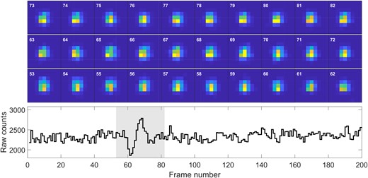
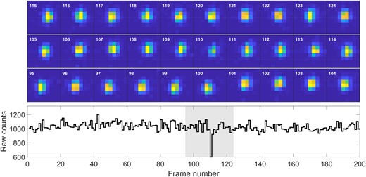
Raw counts and cutouts for the occultation candidate of 2020 July 1. The cutouts are set to the same dynamic range, showing that the dimming and brightening is not an artifact of the photometric reduction, but a feature of the underlying pixel measurements.
The MCMC fit to the light curve yielded poor fits, probably due to the asymmetric and undulating shape of the light curve (see Fig. A2). It would perhaps be more useful to fit this event with models of a binary occulter, but such modelling is more complicated and computationally demanding. Also, due to the similarity between this event and other false-positives we decided to keep the analysis simple. We ran 50 chains with 104 steps (following 104 steps as burn-in), as discussed in Section 3.1. Nine chains converged (were not rejected), with a clearly bi-modal distribution.
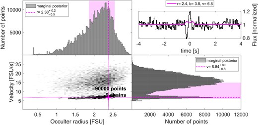
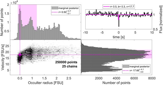
Results of an MCMC analysis (see Section 3.1) for the occultation candidate of 2020 July 1. The lower-left panel shows the posterior, marginalized over the impact parameter, time offset and stellar size, while the top-left and bottom-right panels show the marginalized posteriors leaving only occulter radius and velocity, respectively. The pink, dotted lines and cross show the most likely (best-fitting) value in the two parameters, although the range of likely values includes many other combinations of radius and velocity, as shown by the pink shaded areas that highlight the smallest interval containing 68 per cent of the posterior. The top-right panel shows the raw light curve and the best template (in pink), using the best-fitting parameters described above.
The lower cluster of chains at low velocities (v ≈ 6.8 FSU s−1 ≈ 8.8 km s−1) is inconsistent with the observation’s transverse velocity of 27.2 km s−1. The top cluster has higher velocities, but is also less dense. Both distributions have most of their mass at values of r > 2 FSU, i.e. ≈2.5 km. The large radii reflects the strong changes in the flux over many frames, which is hard to achieve with a small occulter. This, along with the high ecliptic latitude of the event, strengthens our conclusion that this event is a false-positive, caused either by the atmosphere or by instrumental effects.
One way to test if an event is due to spurious atmospheric noise or bad pixels is to look at the number of flux values that are dramatically different from the mean (flux outliers, see Section 3.3). We show the number of outliers found for each star in the top panel of Fig. A3. We see that 90 per cent of the stars have less than 22 outliers in that time range. The candidate star has 25 outliers which puts it in the top 90 per cent of the stars in terms of number of outliers, but is not dramatically different from stars of similar brightness. This indicates the cause of the event is not likely an instrumental effect. We also show the histogram of the flux values for the candidate star, along with a fit to a Gaussian, in the bottom-left panel, highlighting the outlier distribution.
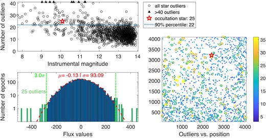
Outlier analysis (see Section 3.3) for the occultation candidate of 2020 July 1. The top panel shows the number of outliers for each star as black circles as a function of each stars’ instrumental magnitude (with an arbitrary zero point). A few stars with outliers above the maximum value in this plot were replaced with black triangles, which helps focus the plot on the occultation star’s range of outliers. The red pentagon shows the position of the candidate star. The blue, horizontal, dashed line shows the 90th percentile, equal to 22 outliers. The bottom-left panel shows the histogram of the flux values as blue bars, the 3σ limits used to find outliers as green, dotted, vertical lines, and the fit to a Gaussian as a red, dashed line. The occultation star has 25 outliers, which is above the 90th percentile but does not seem to be an extreme value compared with other bright stars on the left side of the top panel. The bottom-right panel shows the number of outliers for stars as a function of their pixel coordinates on the focal plane. Large circles represent stars with more outliers than the 90th percentile. The candidate star is marked with a red pentagon. There is no clustering of ‘bad stars’ close to the candidate star.
In the bottom-right panel of Fig. A3 we plot the position of each star on the focal plane, colour coding the marker for each star based on the number of outliers it has. This allows us to visualize any clustering of bad light curves, perhaps indicating local phenomena. In this case, there is some cluster of bad fluxes around x, y = 1000, 2000 but this area is not close to the candidate star, marked with a red pentagon. This again indicates it is less likely that this event is due to local instrumental effects.
Finally, in Fig. A4 we show the fluxes of the nearest neighbouring stars, out of stars with photometric S/N > 5 (see Section 3.2). The light curves do not seem to show similar flux variations as the occultation star, which weakens the hypothesis that this event is atmospheric.
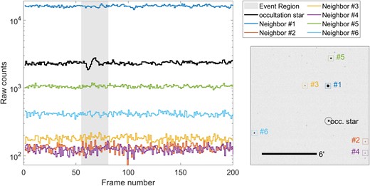
Flux values for nearby stars around the time of the event of 2020 July 1. There does not seem to be any evidence of flux changes in any of the nearby stars during the 8 s period surrounding the event.
A2 Occultation candidate 2021 April 1
This event is a single-frame occultation candidate. The shape of the light curve, as well as the cutout images around the time of the event are shown in Fig. A5.
Raw counts and cutouts for the occultation candidate of 2021 April 1. The cutouts are set to the same dynamic range, showing that the dimming is not an artifact of the photometric reduction, but a feature of the underlying pixel measurements.
The MCMC fit to this event follows the same methods as used for all events (see Section 3.1 and Appendix A1). The posterior distribution, shown in Fig. A6, does not converge on a single peak but traces a wide swath of the parameter range. Most striking is the low probability given to low velocities (v < 5 FSU s−1). At very low transverse velocities, the events are expected to be wide, such that even at 10 Hz sampling they should affect multiple frames. If the KBO occulter is not moving in retrograde, the total transverse velocity should be even lower, making it more unlikely to appear as a single frame event. If the KBO is moving in retrograde, the total transverse velocity could instead be in the range of 10–15 FSU s−1, which is consistent with the event light curve.
Results of an MCMC analysis (see Section 3.1) for the occultation candidate of 2021 April 1. The panels are the same as in Fig. A2. The posterior distribution is spread out over a large part of the parameter space, but does not have much overlap with low velocities (the Earth’s projected velocity for this event is 4.0 km s−1). The best-fitting light curve does not reproduce the depth of the single-frame dip, and requires a velocity of 17.66 FSU s−1, i.e. ≈23 km s−1.
An outlier analysis of the star’s long-term light curve, as described in Section 3.3 reveals that this star does not display a large number of outliers, with 21 outliers in the time range of 4000 frames around the event. Compared with other stars this is not above average.
We also check if other stars nearby the event star are affected by any transient dimming. The results for four nearby stars with S/N > 5 are shown in Fig. A7. We see a suspicious single frame dimming in star #1, but no other obvious transient events on any of the other stars.
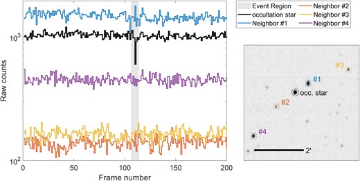
Flux values for nearby stars around the time of the event of 2021 April 1. There is a small decrease in the flux of the most nearby star (#1, blue line), but no other strong dimming events is seen in other stars during the 20 s period surrounding the event.
This event is hard to classify due to the dimming being confined to a single frame. The low velocity of the observations makes it unlikely to be a true occultation event with such a short duration. However, looking at the number of outliers and nearby stars we see no evidence for instrumental or atmospheric effects. This event, along with the next candidate observed only 2 d later, remain questionable, single-frame events.
A3 Occultation candidate 2021 April 3
Similar to the event of 2021 April 1, this event also shows a dimming on a single frame. The cutout images show a clear dimming which is not due to the photometric reduction, as shown in Fig. A8.
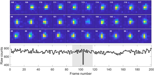
Raw counts and cutouts for the occultation candidate of 2021 April 3. The cutouts are set to the same dynamic range, showing that the dimming is not an artifact of the photometric reduction, but a feature of the underlying pixel measurements.
The MCMC posterior is consistent with a wide range of values for the occulter radius, r, but is fairly limited to high velocities 17 < v < 22.5 FSU s−1 (22 < v < 29 km s−1). This seems wholly inconsistent with the observed transverse velocity of these observations, even for a retrograde, eccentric occulter.
Similarly to the previous event, there is not a substantial number of outliers for the light curve of this star in the 4000 frames around the event. The neighbour stars’ light curves also do not show any substantial transients in the flux of any stars in the few arcmin around the event star. While we do not see any direct evidence for an instrumental or atmospheric disturbance that could explain the dimming, the fact that both this and the event 2 d before show a single-frame dimming at a field with low expected transverse velocities make it improbable that these two events are due to real occultations.
A4 Occultation candidate 2021 April 11
This event is a multiframe occultation candidate, composed of two dimming frames on either side of a relatively bright middle three frames. The shape of the light curve, as well as the cutout images around the time of the event are shown in Fig. A10. The shape is reminiscent of occultations with strong diffraction effects, where in this case the middle brightening, also known as the Poisson peak, is brighter than the edges of the light curve right before and after the dimming frames.
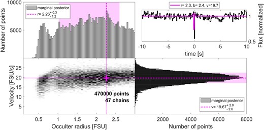
Results of an MCMC analysis (see Section 3.1) for the occultation candidate of 2021 April 3. The panels are the same as in Fig. A2. The posterior distribution is spread out over a large range in r, but a rather limited range of high velocities (≈25.5 ± 3.5 km s−1). By comparison, the Earth’s projected velocity is 5.0 km s−1.
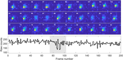
Raw counts and cutouts for the occultation candidate of 2021 April 11. The cutouts are set to the same dynamic range, showing that the dimming is not an artifact of the photometric reduction, but a feature of the underlying pixel measurements.
The MCMC fit to this event follows the same methods as used for all events (see Section 3.1 and Appendix A1). The posterior distribution, shown in Fig. A11, follows a bi-modal distribution, with two spots at different velocities. The larger spot, centred at r = 0.6 FSU and v = 14 FSU s−1, strongly constrains the parameters of this event, mostly due to the presence of the Poisson peak and the many frames of the occultation. While this is marginally consistent with the observed Earth velocity of 7.3 FSU s−1, it once again requires a retrograde occulter to match the width of the light curve. We also notice that the best-fitting light curve, shown in pink on the top-right panel of Fig. A11, does not reproduce the strong Poisson peak of the event. Manually running some simulations, we conclude that a Poisson peak that is equally as bright as the ingress/egress fringes of the occultation is only possible when the impact parameter is close to zero, which is not a particularly likely value.
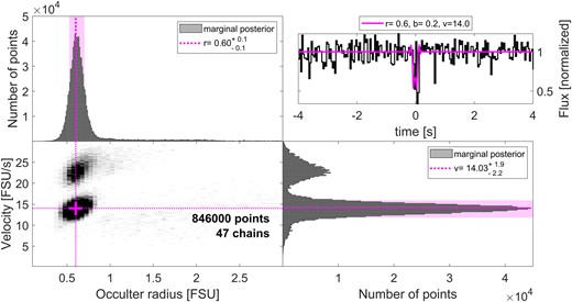
Results of an MCMC analysis (see Section 3.1) for the occultation candidate of 2021 April 11. The panels are the same as in Fig. A2. There are two clusters for the two-dimensional (2D) posterior distribution. The denser one, at a lower velocity of ≈18.2 ± 3 km s−1, is only marginally consistent with the Earth’s transverse velocity of 9.5 km s−1, if we assume a retrograde occulter. The strong Poisson peak in the event light curve is not matched by the best-fitting template, which requires a small impact parameter which is not in itself very likely.
An outlier analysis of the star’s long-term light curve, as described in Section 3.3 is shown in Fig. A12. This star’s long-term light curve (spanning 4000 frames, or 400 s, around the event) shows an unusually high number of dimming outlier events. A cluster of stars nearby on the sensor are seen to have a high number of outliers (seen on the bottom-right panel) which indicates some problem with that area of the detector, either due to defocus, vignetting, or a bad match of the photometric aperture to the star positions. The event star has 79 outlier frames in that time range, mostly dimming frames, while the rest of the stars’ 90th percentile is only 33 outliers. This result makes it highly likely that the dimming is caused by an instrumental effect, not a physical occultation.
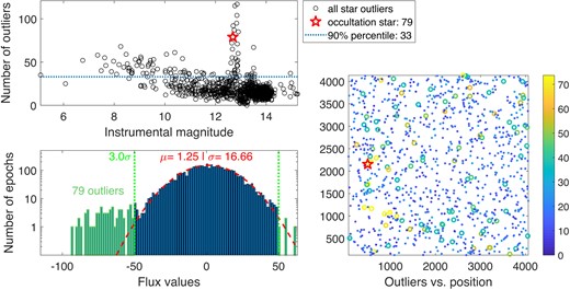
Outlier analysis (see Section 3.3) for the occultation candidate of 2021 April 11. The panels are the same as in Fig. A3. The occultation star has 79 outliers, which is more than double the 90th percentile (of 33 outliers). On the bottom-right panel we see the star appears to be in a region with many high-outlier stars, which is indicative of an instrumental or atmospheric origin for the event.
We also check if other stars nearby the event star are affected by any transient dimming. The results for four nearby stars with S/N > 5 are shown in Fig. A13. There is some evidence that the stars #1 and #4, shown as the blue and purple lines, respectively, also show strong variability on similar time-scales as the event star. This is consistent with an instrumental effect but also with an atmospheric event that affected some of the stars nearby.
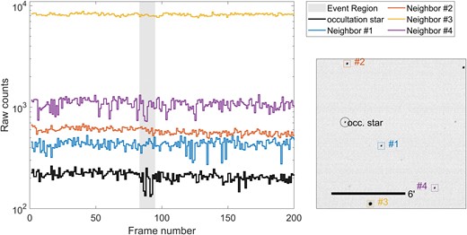
Flux values for nearby stars around the time of the event of 2021 April 11. Stars #1 and #4, shown as blue and purple lines, show strong variability, indicating an atmospheric or instrumental origin.
A5 Occultation candidate 2021 April 12
This event is a multiframe occultation candidate, composed of one and two dimming frames before and after a normal brightness, single middle frame. The shape of the light curve, as well as the cutout images around the time of the event are shown in Fig. A14. The shape is reminiscent of occultations with strong diffraction effects. It has fewer dimming frames, and a shorter and less prominent middle part, compared with the event detected only 1 d before it.
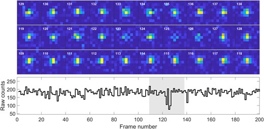
Raw counts and cutouts for the occultation candidate of 2021 April 12. The cutouts are set to the same dynamic range, showing that the dimming is not an artifact of the photometric reduction, but a feature of the underlying pixel measurements.
The MCMC fit to this event follows the same methods as those used for all events (see Section 3.1 and Appendix A1). The posterior distribution, shown in Fig. A15, follows a bi-modal distribution, with one small spot at low velocity and radius, and another large distribution at higher velocities that spans most of the allowed range for the occulter radius. We also notice that the best-fitting light curve, shown in pink on the top-right panel of Fig. A15, does not reproduce the Poisson peak of the event.
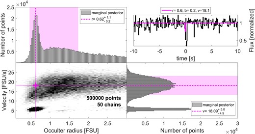
Results of an MCMC analysis (see Section 3.1) for the occultation candidate of 2021 April 12. The panels are the same as in Fig. A2. There are two clusters for the 2D posterior distribution. The smaller one, at a lower velocity of ≈8 ± 2 km s−1, is consistent with the Earth’s transverse velocity of 9.3 km s−1, but the velocity of the upper cluster of ≈24 ± 6.5 km s−1 is too high to be consistent. None of the points in either distribution manages to reproduce the single-frame Poisson peak of this event, even with an impact parameter set to zero.
We check whether a combination of parameters from one of these two distributions fits the light curve more successfully than using the ‘best-fitting’ parameters, which are calculated using the velocity of the larger distribution and the radius of the smaller one. We chose the central values of either distribution, along with b = 0 and R = 0.38 FSU (the best fit to the star’s Gaia magnitudes). We show the resulting light curve templates, along with the real event counts in Fig. A16. It is clear that neither of these templates can reproduce the central peak in the raw light curve. Even at negligible impact parameter values, the low frame rate (10 Hz) will wash out the brightening at the centre of the illumination pattern, such that it would not show a strong Poisson peak. It is much more likely that the event originates from an instrumental or atmospheric effect.
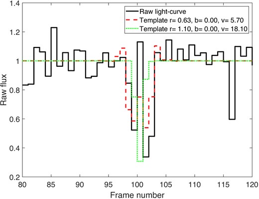
Comparison of occultation parameters to the light curve of the event at 2021 April 12. We chose the central values from the bi-modal posterior presented in Fig. A15, and show the resulting templates, setting both to R⋆ = 0.38, the star’s best-fitting value, and b = 0, the optimal impact parameter to recreate the strong Poisson peak in this light curve. The low-velocity template still cannot recreate the Poisson peak, while the high-velocity template completely skips that part and only produces a few dimming frames.
An outlier analysis of the star’s long-term light curve, as described in Section 3.3 is shown in Fig. A17. As was the case for the event of 2021 April 11, this star’s long-term light curve (spanning 4000 frames, or 400 s, around the event) shows an unusually high number of dimming outlier events. The event star has 62 outlier frames in that time range, mostly dimming frames, while the rest of the stars’ 90th percentile is only 30 outlier frames. This result makes it highly likely that the dimming is caused by an instrumental effect, not a physical occultation.
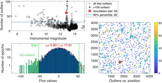
Outlier analysis (see Section 3.3) for the occultation candidate of 2021 April 12. The panels are the same as in Fig. A3. The occultation star has 62 outliers, which is more than double the 90th percentile (of 30 outliers). On the bottom-right panel we see the candidate star does not seem to be close to any overabundance in high-outlier stars. However, just the number of outliers it has in the long-term light curve indicates an instrumental effect is the likely cause of the event.
We also check if other stars nearby the event star are affected by any transient dimming. The results for four nearby stars with S/N > 5 are shown in Fig. A18. There is some evidence that star #4, shown as the purple line, also shows strong variability on similar time-scales as the event star. This is consistent with an instrumental effect but also with an atmospheric event that affected some of the stars nearby.
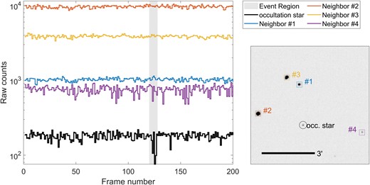
Flux values for nearby stars around the time of the event of 2021 April 12. Star #4, shown as a purple line, shows strong variability throughout the event time. Other stars do not show strong variability, so it is hard to draw conclusions based on the nearby stars.
A6 Occultation candidate 2021 April 16
This event is a multiframe occultation candidate, composed of four consecutive frames of lower flux values. It is more promising as a true occultation candidate than the previous events, although still far from being a definite detection. The shape of the light curve, as well as the cutout images around the time of the event are shown in Fig. A19. The shape of the light curve does not show any diffraction effects, and in fact the steep drop-off of the intensity of light at the beginning and end of the dip is surprising, given the high cadence of the observations.
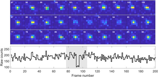
Raw counts and cutouts for the occultation candidate of 2021 April 16. The cutouts are set to the same dynamic range, showing that the dimming is not an artifact of the photometric reduction, but a feature of the underlying pixel measurements.
The MCMC fit to this event follows the same methods as used for all events (see Section 3.1 and Appendix A1). The posterior distribution, shown in Fig. A20, shows a rather narrow peak centred around r = 0.6 FSU and v = 16.3 FSU s−1, and a wider range of points that likely arise from chains that are not fully converged. The majority of the probability, however, is densely concentrated, with radius and velocity that are consistent with an occultation by a small KBO.
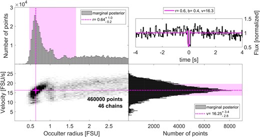
Results of an MCMC analysis (see Section 3.1) for the occultation candidate of 2021 April 16. The panels are the same as in Fig. A2. The majority of the posterior probability is focused on a small region of the parameter space which is consistent with the transverse velocity of the observed field. The size of the occulter is consistent with a small KBO (r ≈ 0.6 FSU = 0.9 km).
While the parameter estimation described above seem to be consistent with a real occultation with the correct transverse velocity, an outlier analysis quickly shows that this is not likely to be the cause of the event. The results of such an analysis, as described in Section 3.3 is shown in Fig. A21. As was the case for the events of 2021 April 11 and 12, this star’s long-term light curve (spanning 4000 frames, or 400 s, around the event) shows an unusually high number of dimming outlier events. The event star has 119 outlier frames in that time range, mostly dimming frames, while the rest of the stars’ 90th percentile is only 34 outlier frames. This result makes it most likely that the dimming is caused by an instrumental effect, not a physical occultation.
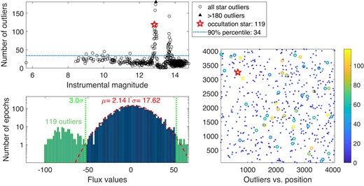
Outlier analysis (see Section 3.3) for the occultation candidate of 2021 April 16. The panels are the same as in Fig. A3. The occultation star has 119 outliers, which is almost three times the 90th percentile (of 34 outliers). In the bottom-right panel, we see that the candidate star does not seem to be close to any overabundance in high-outlier stars. However, the number of outliers it has in the long-term light curve indicates an instrumental effect is the likely cause of the event.
We also check if other stars nearby the event star are affected by any transient dimming. The results for four nearby stars with S/N > 5 are shown in Fig. A22. There is some evidence that star #1 (the closest one, shown as the blue line), also shows strong variability on similar time-scales as the event star. This is consistent with an instrumental effect but also with an atmospheric event that affected some of the stars nearby. However, it should be noted that the closest stars are more than 10 arcmin from the event star, so may not be good indicators for variability for this event.
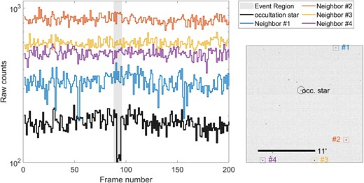
Flux values for nearby stars around the time of the event of 2021 April 16. Star #1, shown as a blue line, shows strong variability throughout the frames surrounding the event. Other stars do not show strong variability, so it is hard to draw conclusions based on the nearby stars.
A7 Occultation candidate 2021 September 14
This event is a multiframe occultation candidate, composed of four consecutive frames of lower flux values, of which one is slightly brighter, and at least another frame where the flux exceeds the average. It is the only event in 2021 that was not detected in the first two-and-a-half weeks of April, and it looks more consistent with a real occultation than all other events. It does not, however, appear to be a clear true detection or a definite false-positive. The shape of the light curve, as well as the cutout images around the time of the event are shown in Fig. A23. The shape of the light curve is asymmetric, with a clear brightening after an initial dip. Such light curves often arise from binary or elongated occulters, according to simulations (see Nir et al. 2023).
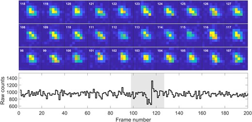
Raw counts and cutouts for the occultation candidate of 2021 September 14. The cutouts are set to the same dynamic range, showing that the dimming and brightening are not artifacts of the photometric reduction, but features of the underlying pixel measurements.
The MCMC fit to this event follows the same methods as used for all events (see Section 3.1 and Appendix A1). The posterior distribution, shown in Fig. A24, shows a rather narrow peak centred around r = 0.5 FSU and v = 5.7 FSU s−1, and another region with similar velocity and a wider occulter radius range. The majority of the probability, however, is densely concentrated, with radius and velocity that are consistent with an occultation by a small KBO at a low velocity. A light curve template associated with such an occultation is shown in the top-right panel of Fig. A24, which fits the dip in flux fairly successfully, but does not account for the small brightening in the middle of the dip or the larger brightening after it. The inferred velocity is inconsistent with a KBO, which will require a transverse velocity of ≈10 FSU s−1 = 13 km s−1.
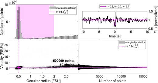
Results of an MCMC analysis (see Section 3.1) for the occultation candidate of 2021 September 14. The panels are the same as in Fig. A2. The majority of the posterior probability is focused on a small region of the parameter space with low occulter radii (≈0.65 km) and velocities (≈7.5 ± 0.1 km s−1), the latter being inconsistent with the field’s transverse velocity of 20.3 km s−1.
An outlier analysis, as described in Section 3.3 does not reveal an overabundance of flux outliers in the 4000 frame (400 s) time span around the event. The star’s light curve contains 21 outliers in that time, less than the 90 per cent percentile of 29, and similar to the mean of stars of that brightness.
We also check if other stars nearby the event star are affected by any transient dimming. The results for four nearby stars with S/N > 5 are shown in Fig. A25. There is some evidence that star #1 (the closest one, shown as the blue line), changes brightness within about 10 frames (1 s) from the time when the candidate event occurs. Other stars within a few arcmin do not show any unusual variability. While the nearby star’s behaviour is suspicious, it does not appear similar in nature to the dimming and brightening of this event.
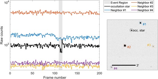
Flux values for nearby stars around the time of the event of 2021 September 14. Star #1, shown as a blue line, seems to drop in flux right before the candidate occultation occurs, but remains at a ‘low state’ for the remaining frames in that batch. The shape of the two changes in flux is not similar, and it is unclear what sort of transient effect could cause both. Other stars do not show strong variability, so it is hard to draw conclusions based on the nearby stars.
A8 Candidate summary
The seven candidate occultations presented here are all ruled out for one reason or another. Some are clearly false-positives, such as events with many outliers in the long-term light curves. Others seem likely to be atmospheric, such as the events of 2020 July 1 or 2021 September 14 that show both decrease and increase of flux, appearing ‘flare-like’ which makes them suspiciously similar to the flare events presented in Appendix B. Two events are single-frame events where there is insufficient information to confirm or rule out the events, but the low transverse velocity makes them unlikely to be KBO occultations.
We summarize the properties of all seven candidates in Table 1. One event (2020 July 1) is flare-like and off-ecliptic. Three events have many outliers (2021 April 11, 12, and 16). Three events have inconsistent transverse velocities (2020 July 1, 2021 April 1 and 3, and September 14). It is clear that none of the candidates is fully consistent with what we expect from a KBO occultation.
We thus conclude that none of the candidate events are caused by KBO occultations. We calculate the limits on the number density based on this null result in Section 5.1. The variety of light-curve morphologies should be taken as an indication for the many types of false-positives that could arise in such a search for fast transients under atmospheric conditions.
APPENDIX B: FLARE EVENTS
In addition to finding occultation events, our pipeline was also sensitive to ‘flares’, i.e. events where the flux is mostly increasing, rather than dimming. Many such events were detected and flagged as satellite glints or tracks.
After removing all obvious satellites we detected 41 potential flares. Careful inspection of the cutout images has ruled out a further 11 events where the satellite was seen glinting close to the edge of the cutout or just as a faint moving object relative to the star. The remaining 30 flares could be due to (1) more satellites that somehow were visible only near the star; (2) occultations where a bright diffraction fringe passes over the observer; (3) atmospheric fluctuations that momentarily focus the star’s light; and (4) some unknown transient phenomena that increases the flux of stars for less than a second. The colour–magnitude position of all 30 flares, and the occultation-like events, is shown in Fig. B1, superimposed on the distribution of colours and magnitudes of stars in Gaia DR3. The events are all on relatively bright stars, which could be interpreted as a detection bias or as an indication that these are instrumental/atmospheric artefacts. Both kinds of events do not seem associated with a particular population of active stars. The light curves for all 30 flares is shown in Fig. B2 on arbitrary flux axes (normalized to the median of each light curve).
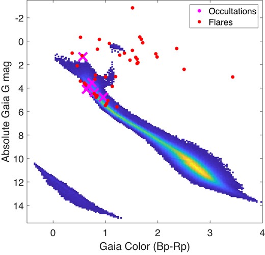
The colour–magnitude of occultation-like events (magenta crosses) and flares (red circles) superimposed on the density map of stars from Gaia DR2. Events appear to occur on brighter stars, which could be a detection bias or an indication that these are artifacts. Neither type of event seems to be associated with a population of active stars. Absorption was used for all stars with a known absorption from the Gaia catalogue. One occultation-like event and one flare are not shown as the underlying star did not have positive parallax measured in the catalogue.
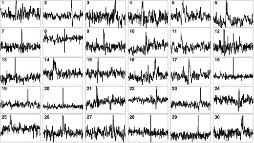
Light curves for all flares detected in the 2020–2021 observing seasons. These events remain after removing all visible indications of source motion, caused by satellite glints. The flux scale is normalized to the median of each light curve, to show the morphology of the flares. Information about each individual flare is given in Table B1.
It is likely that some of the flares are due to satellite glints that perfectly align with the star’s position and do not reflect any additional light before or after crossing close to the star’s position. Nir et al. (2021a) reported such glints, with a rate of 1.3 × 10⁻⁷ glints per hour per arcsec squared, for glints brighter than 11th magnitude. With ≈106 star-hours, and the images of stars with a typical FWHM of ≈5 arcsec, we can estimate there would be ≈3 satellite glints in our data. The stars in our sample are commonly dimmer than 11th magnitude. If the magnitude distribution of glints does not drop off after the 11th magnitude, there could potentially be even more glints, with similar flux to the stars they are on.
Bright diffraction fringes can also appear as flux increases, usually accompanied by dimming before or after the flare. This is indeed seen in some simulated light curves (see Nir et al. 2023). However, this is relatively rare, compared with normal (dimming) occultations. Looking at simulated occultation templates within the range of occulter radii 0.3 < r < 3 FSU and impact parameters 0 < b < 2 FSU, we find less than 30 per cent of events have more positive flux points than dimming points. Therefore, even if a few events are due to this effect, there should be × 3 more dimming than flaring occultations in our data. Binary or elongated occulters have more likelihood to produce flux increases, but even then most events would also produce dimming, unless the major axis of the occulting body (or bodies) is perfectly aligned relative to the direction of motion, which is not particularly likely (see Nir et al. 2023).
Atmospheric phenomena remains a viable explanation for at least some of the flare events, and also most of the occultation events discussed in the previous section. Inspecting histograms of outlier flux values does not immediately show a long tail of flux variations that would be expected from random atmospheric fluctuations. Observations with multiple telescopes could help conclude if these are extreme atmospheric events or caused by physical phenomena outside the Earth.
Finally, although less likely, we cannot rule out that these are actual unknown transient phenomena occurring at the star or in the light’s path through the Solar system. We find this explanation most unlikely.
A summary of the properties of the flare events is given in Table B1. We do not apply the additional parameter estimation or outlier analysis for these events, but we do note the flares that show some dimming in the light curve that makes them similar to occultation events.
Summary of flare events. Most of the columns are the same as in Table 1. The columns for parameter ranges, neighbours, and outlier numbers have been removed as these events did not get the full processing as the occultation candidates. The column for flare-like is replaced with ‘occultation-like’, where a flare would be occultation-like if it displays a pronounced dip in the flux, in addition to the brightening. The first column is a serial number which refers to the numbers of the panels in Fig. B2.
| Number | Event time (UTC) | Coordinates | β | Event S/N | MG | Teff | R⋆ | Phot. S/N | f | FWHM | A.M. | VT | Occultation-like |
|---|---|---|---|---|---|---|---|---|---|---|---|---|---|
| (hh:mm:dd±dd:mm:ss) | (deg) | (○K) | (FSU) | (Hz) | (arcsec) | (kms−1) | |||||||
| 1 | 2020-07-25 19:19:23 | 18:05:31.0-19:56:44.6 | 3.0 | 7.91 | 12.11 | 4995 | 0.4 | 6.63 | 25 | 4.79 | 1.59 | 27.1 | No |
| 2 | 2020-07-25 21:03:36 | 18:05:38.1-21:21:22.0 | 3.0 | 7.50 | 10.58 | 3977 | 2.5 | 8.68 | 25 | 5.72 | 1.76 | 27.1 | Yes |
| 3 | 2020-07-25 22:31:47 | 18:05:22.7-21:40:25.3 | 3.0 | 8.02 | 8.26 | 5867 | 2.0 | 10.62 | 25 | 5.41 | 2.51 | 27.1 | No |
| 4 | 2020-08-04 20:01:05 | 20:17:56.1-17:40:23.3 | 1.9 | 7.72 | 10.16 | 7762 | 0.5 | 13.86 | 25 | 5.28 | 1.58 | 25.7 | No |
| 5 | 2020-08-06 20:19:27 | 20:23:21.9-17:25:42.6 | 1.9 | 7.52 | 13.01 | 7656 | 0.1 | 5.72 | 25 | 5.89 | 1.52 | 25.6 | No |
| 6 | 2020-08-10 19:57:36 | 18:08:23.8-19:11:38.9 | 3.0 | 8.05 | 10.95 | 5802 | 0.8 | 12.20 | 25 | 4.76 | 1.75 | 24.9 | No |
| 7 | 2020-08-10 18:00:40 | 20:18:39.6-16:26:38.6 | 1.9 | 9.10 | 12.03 | 4134 | 0.9 | 5.31 | 25 | 6.01 | 2.13 | 25.4 | No |
| 8 | 2020-08-28 20:00:47 | 19:40:18.4+40:13:22.5 | 59.2 | 8.25 | 12.72 | 5643 | 0.3 | 4.14 | 25 | 7.21 | 1.05 | 16.8 | No |
| 9 | 2020-09-10 17:57:28 | 18:08:21.0-19:32:50.3 | 3.0 | 7.59 | 11.71 | 5838 | 0.9 | 7.29 | 25 | 9.20 | 1.75 | 21.0 | No |
| 10 | 2020-09-10 18:01:00 | 18:09:03.3-21:23:12.6 | 3.0 | 8.20 | 11.59 | 7117 | 0.3 | 7.85 | 25 | 5.76 | 1.77 | 21.0 | No |
| 11 | 2020-09-10 18:01:36 | 18:08:41.6-20:05:13.8 | 3.0 | 8.23 | 7.39 | 4332 | 5.3 | 10.31 | 25 | 8.46 | 1.77 | 21.0 | No |
| 12 | 2021-04-02 20:01:38 | 07:58:46.1+19:56:51.8 | −1.5 | 7.51 | 11.30 | 4733 | 0.8 | 14.61 | 10 | 7.51 | 1.38 | 2.3 | No |
| 13 | 2021-04-03 17:14:36 | 06:33:20.5+20:28:52.9 | −1.7 | 8.21 | 10.33 | 4613 | 1.3 | 28.12 | 10 | 5.27 | 1.11 | 5.0 | No |
| 14 | 2021-04-03 17:37:16 | 06:34:43.4+20:45:41.8 | −1.7 | 7.89 | 11.11 | 6738 | 0.6 | 22.06 | 10 | 6.59 | 1.16 | 5.0 | No |
| 15 | 2021-04-21 00:08:59 | 18:09:13.2-20:27:20.7 | 3.0 | 13.53 | 12.32 | 3671 | 2.0 | 6.36 | 10 | 6.33 | 1.82 | 22.9 | Yes |
| 16 | 2021-06-01 01:20:54 | 18:05:14.0-19:35:31.1 | 3.0 | 8.16 | 10.92 | 4236 | 1.6 | 13.82 | 10 | 8.35 | 1.99 | 28.3 | No |
| 17 | 2021-06-04 20:02:52 | 15:43:03.3-19:41:04.7 | 0.2 | 7.61 | 10.45 | 7050 | 0.7 | 19.90 | 10 | 5.23 | 1.57 | 25.7 | No |
| 18 | 2021-06-06 21:49:23 | 18:04:02.3-21:09:07.5 | 3.0 | 7.61 | 10.63 | 7154 | 0.4 | 19.23 | 10 | 4.70 | 1.65 | 28.7 | No |
| 19 | 2021-06-11 22:09:13 | 18:05:02.3-20:32:03.4 | 3.0 | 7.52 | 10.79 | 5773 | 0.6 | 12.32 | 10 | 5.15 | 1.59 | 29.0 | No |
| 20 | 2021-06-15 22:21:43 | 16:57:45.0-25:51:04.0 | −1.7 | 7.61 | 12.83 | 4391 | 0.5 | 10.57 | 10 | 5.83 | 1.89 | 28.6 | No |
| 21 | 2021-06-19 19:49:35 | 18:06:54.6-21:05:26.5 | 3.0 | 9.12 | 12.93 | 3670 | 1.9 | 6.55 | 10 | 4.85 | 1.96 | 29.3 | No |
| 22 | 2021-06-27 20:14:20 | 15:35:29.1-19:49:50.7 | 0.2 | 13.60 | 12.98 | 5086 | 0.4 | 12.16 | 10 | 5.85 | 1.67 | 23.4 | Yes |
| 23 | 2021-07-07 19:41:44 | 18:05:31.8-20:04:56.7 | 3.0 | 7.87 | 11.40 | 4360 | 1.2 | 18.42 | 10 | 4.90 | 1.67 | 28.8 | No |
| 24 | 2021-07-08 19:42:11 | 18:00:23.5-20:34:21.0 | 3.0 | 7.98 | 10.65 | 5314 | 0.8 | 25.22 | 10 | 6.50 | 1.66 | 28.8 | No |
| 25 | 2021-07-10 22:48:07 | 22:02:33.5-10:29:14.2 | 1.3 | 7.53 | 12.28 | 4973 | 0.4 | 13.22 | 10 | 6.59 | 1.48 | 17.5 | No |
| 26 | 2021-07-10 22:49:37 | 22:03:43.3-09:31:33.7 | 1.3 | 8.06 | 10.05 | 4127 | 2.3 | 16.47 | 10 | 5.11 | 1.48 | 17.5 | No |
| 27 | 2021-07-12 20:18:34 | 18:04:03.3-21:41:45.1 | 3.0 | 9.79 | 13.58 | 5350 | 0.3 | 8.17 | 10 | 8.10 | 1.59 | 28.5 | No |
| 28 | 2021-07-14 22:14:11 | 18:07:12.1-19:48:49.8 | 3.0 | 13.76 | 14.12 | 4882 | 0.3 | 7.11 | 10 | 6.72 | 1.89 | 28.3 | Yes |
| 29 | 2021-07-16 22:08:51 | 18:05:12.4-19:48:52.8 | 3.0 | 13.78 | 13.96 | 5993 | 0.2 | 7.36 | 10 | 5.91 | 1.91 | 28.1 | No |
| 30 | 2021-07-28 18:41:55 | 18:22:56.3-24:48:54.5 | −1.6 | 7.69 | 12.70 | 4311 | 0.7 | 6.70 | 10 | 6.19 | 1.83 | 27.4 | No |
