


ABSTRACT
Using VLT/MUSE integral-field spectroscopic data for the barred spiral galaxy NGC 1097, we explore techniques that can be used to search for extended coherent shocks that can drive gas inflows in centres of galaxies. Such shocks should appear as coherent velocity jumps in gas kinematic maps, but this appearance can be distorted by inaccurate extraction of the velocity values and dominated by the global rotational flow and local perturbations like stellar outflows. We include multiple components in the emission-line fits, which corrects the extracted velocity values and reveals emission associated with AGN outflows. We show that removal of the global rotational flow by subtracting the circular velocity of a fitted flat disc can produce artefacts that obscure signatures of the shocks in the residual velocities if the inner part of the disc is warped or if gas is moving around the centre on elongated (non-circular) trajectories. As an alternative, we propose a model-independent method which examines differences in the LOSVD moments of H α and [N II]λ6583. This new method successfully reveals the presence of continuous shocks in the regions inward from the nuclear ring of NGC 1097, in agreement with nuclear spiral models.
1 INTRODUCTION
Gas inflows play an important role in the evolution of galaxies: they enhance nuclear star formation (SF) (Ellison et al. 2011; Prieto et al. 2019), which can cause starbursts in nuclear rings (Heller & Shlosman 1994; Mazzuca et al. 2008) and change the morphology of the central regions by creating substructures (e.g. gaseous and stellar discs, rings) (Shlosman, Frank & Begelman 1989; Athanassoula 1992; Martini et al. 2003; Kim et al. 2012; Sormani, Binney & Magorrian 2015). Further, the gas reaching the very centre can trigger active galactic nuclei (AGNs) (Davies et al. 2014; Audibert et al. 2020) and lead to highly energetic feedback (Prieto, Maciejewski & Reunanen 2005; Davies et al. 2014; Audibert et al. 2019). Outflowing gas from AGN feedback can in turn rapidly suppress SF and cause quenching (Man et al. 2019; Donnari et al. 2021). Hence, to understand the structural evolution of the galaxies, it is important to understand the role of the inflowing gas.
Mechanisms triggering gas inflow on various scales have been a prominent focus of many observational and theoretical studies (Sanders & Huntley 1976; Athanassoula 1992; Emsellem, Goudfrooij & Ferruit 2003; Maciejewski 2004; Fathi et al. 2006; Lin et al. 2013; Fragkoudi, Athanassoula & Bosma 2016; Prieto et al. 2019). Simulations have revealed that non-axisymmetric potentials such as large-scale bars and ovals efficiently transport gas towards the inner kiloparsec (Athanassoula 1992; García-Burillo et al. 2005; Lin et al. 2013; Audibert et al. 2021) by generating torques that put gas clouds on intersecting trajectories. This leads to shocks, in which the gas loses angular momentum and funnels inwards, though the efficiency of this mechanism inside the inner kiloparsec is questioned (Kim et al. 2012). It is also evident from both observations and simulations that central stellar components such as nuclear bars and discs affect the kinematics of the gas (Shlosman 2001; Maciejewski et al. 2002; Fathi et al. 2005), but we require more understanding of mechanisms transferring gas in the nuclear regions of the galaxies.
Shocks in gas that form in response to the gravitational torques of bars and ovals extend over large distances along straight or curved lines, the latter often assuming a spiral shape. Although dust filaments can indicate gas compression in shocks, shock condition implies a rapid change in velocity (Athanassoula 1992; Maciejewski 2004), therefore coherent structures in kinematic maps are best indicators of shocks (Zurita et al. 2004; Fathi et al. 2005; Storchi-Bergmann et al. 2007). In this series of papers, we aim to identify gas inflows by searching for coherent kinematic structures in integral-field spectroscopic observations, which allow us to obtain spectral information over a 2D spatial field-of-view (FoV) of integral field units (IFUs).
We will conduct our search using a diverse sample of galaxies from a multiwavelength imaging and spectroscopic observing campaign Composite Bulges Survey (CBS; Erwin et al., in preparation). CBS focuses on understanding the formation and growth mechanisms of bulges, and the correlation with their host galaxy properties and aims to identify and characterize different forms of nuclear stellar components, from large-scale bars down to nuclear scale discs/rings/bars and nuclear star clusters, of nearby galaxies (Erwin et al. 2021). The sample is a mass- and volume-limited set of 53 disc (S0–Sbc) galaxies with optical and near-IR (NIR) imaging with the Hubble Space Telescope (HST), of which 40 have been observed with the Multi-Unit Spectroscopic Explorer (MUSE) instrument of the Very Large Telescope (VLT). Therefore, benefiting from a diverse galaxy sample, we should be able to determine whether gas inflows in the centres of galaxies occur predominantly in coherent kinematic structures. Moreover, we should be able to examine the connection between different central stellar structures and the presence of coherent kinematic structures indicating inflow.
Tracing the flow of gas in nuclear regions of galaxies has been a challenging task with former generations of IFUs because of their instrumental limitations, such as small fields of view and low spatial resolution. Moreover, in the case of having a low signal-to-noise ratio (SNR), coherent kinematic structures were lost after binning (Fathi et al. 2005, 2006; Storchi-Bergmann et al. 2007). In our study, we predominantly rely on data from MUSE, which with its large, 60 × 60 arcsec2, FoV, fine spatial resolution, and 0.2×0.2 arcsec2 sampling, allows us to capture the nuclear regions of nearby galaxies in great detail. Moreover, MUSE can obtain sufficient SNR for nearby targets, minimizing the need for binning to improve SNR. For our study on gaseous kinematic structures, we prefer not to bin the data to prevent losing spatial information. Hence, in comparison to pioneering studies that suffered from instrumental limitations, advancements of MUSE maximize the prospect of finding coherent kinematic structures.
In this pilot study, we introduce the methodology that we developed to identify coherent kinematic structures in the centres of galaxies, and apply it to the nuclear regions of a galaxy in the CBS sample, NGC 1097 (D = 14.8 Mpc; Freedman et al. 2001, 1 arcsec ≈ 72 pc). NGC 1097 is an SBb galaxy with a strong bar at position angle ∼141° (Prieto et al. 2005) and it contains a prominent star-forming nuclear ring in the inner ∼8–10 arcsec (Bittner et al. 2020). The galaxy hosts a LINER1 type, low-luminosity active galactic nucleus (LLAGN – |$L_{\rm bol}\lesssim 10^{42}\, \rm erg\, s^{-1}$|; Ho 2008) with bolometric luminosity |$L_{\rm bol}=8.6 \times 10^{41}\, \rm erg\, s^{-1}$| (Nemmen et al. 2006). The galaxy is interacting with a companion elliptical galaxy NGC 1097A located to its north-west. Because of its complex characteristics, NGC 1097 has been a prominent focus of many studies (Quillen et al. 1995; Prieto et al. 2005; Fathi et al. 2006; Davies et al. 2009; van de Ven & Fathi 2010; Lin et al. 2013; Bowen et al. 2016; Izumi et al. 2017; Prieto et al. 2019; Legodi, Taylor & Stil 2021).
The flow of the paper is as follows: In Section 2 we present the observations of NGC 1097, and we introduce the data extraction processes for MUSE, including our approach of fitting the gas emission with multiple components. We present our main methodology of finding coherent kinematic structures, and we apply it to the galaxy NGC 1097 in Section 3. We provide the discussion of our findings in Section 4.
2 OBSERVATIONS AND PROCEDURES FOR DERIVING THE LOSVD MOMENTS
2.1 Observations of NGC 1097
MUSE observations of NGC 1097 used in CBS are provided by the TIMER project as a part of observing proposal ID:097.B-0640 (PI: Dimitri Gadotti), carried out in ESO Period 97 on 2016 July 31. The TIMER project studies nearby barred galaxies (D < 40 Mpc) larger than 1 arcmin with stellar masses above 1010 M⊙, brightness threshold of 15.5 B-mag and inclinations smaller than ≈60°, which display prominent central components (e.g. nuclear rings/discs, inner bars). Observations are done in MUSE Wide-Field Mode (WFM), for a nominal wavelength range of 4700–9350 Å. The FoV of WFM encloses an area of 60×60 arcsec2, has a spatial sampling of 0.2 arcsec pixel−1 (Bacon et al. 2010). The point spread function full-width at half-maximum of the observations for NGC 1097 is 0.8 arcsec, which corresponds to a spatial resolution of ∼58 pc. Further details on observations and the data reduction processes, products including stellar kinematics, ages, and metallicities of the sample can be found in Gadotti et al. (2019, 2020) and Bittner et al. (2020). In the left-hand panel Fig. 1, we present a large-scale (360 × 360 arcsec2) image2 of NGC 1097, which reveals the spiral arms on the north and the south, and the companion elliptical galaxy NGC 1097A in the north-west. In the right-hand panel Fig. 1, we present the colour composite image within the inner 60 ×60 arcsec2, constructed from the MUSE data. In both panels, the stellar nuclear ring in the centre and the connection of dust lanes to the nuclear ring are very well resolved.
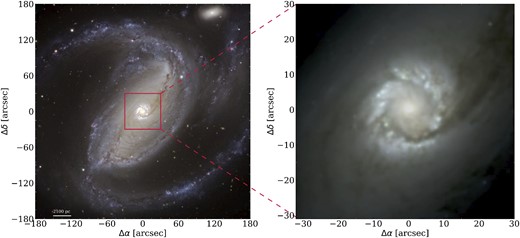
MUSE coverage of NGC 1097. Left-hand panel: Large-scale (360 ×360 arcsec2) image of NGC 1097 taken by VIMOS/VLT. The MUSE coverage of 60 ×60 arcsec2 is highlighted with the red box. Right-hand panel: Colour composite image within the MUSE FoV, constructed by using the MUSE data cube. Images in both panels are centred on the brightest point in the centre. The North is to the top and the East is to the left.
2.2 Extraction of the kinematic data
Spatially resolved spectroscopic data hold a great amount of information, which can be used to probe the fundamental properties of galaxies. To derive emission line fluxes and to extract stellar and ionized gas kinematics from MUSE data, we employ the Data Analysis Pipeline3 (DAP) of the PHANGS collaboration (Emsellem et al. 2022), which is an implementation based on the GIST pipeline (Bittner et al. 2019). DAP is an exceptionally functional software of modular structure, and it employs the commonly used penalized pixel-fitting (pPXF) code (Cappellari & Emsellem 2004) to perform both stellar and emission line analysis. To optimize the processing time of DAP, we discarded the stellar population history module, since it was outside of the scope of this work. A schematic overview of DAP highlighting the main modules, the routines for data extraction, and the products is presented in Fig. 2. A representative spectrum with the pPXF fit for both stellar and emission lines is shown in Fig. 5 (top panel).

Our implementation of the Data Analysis Pipeline. Arrows follow the order of the workflow within the pipeline. Voronoi binned data are transferred to stellar kinematics, extinction (not used), stellar population (not used), and emission line analysis modules, respectively. Note that the emission line analysis can also be performed on single spaxels. In the rightmost blocks, we present the routine used in each module to perform the analysis alongside the derived products.
2.2.1 Deriving stellar line-of-sight velocity distribution moments
We extracted the stellar kinematics in the form of line-of-sight velocity distribution (LOSVD) moments – mean velocity (V), velocity dispersion (σ), and Gauss-Hermite higher order moments (h3 & h4) (van der Marel & Franx 1993). Before deriving the LOSVD moments, the data are resampled on a logarithmic wavelength axis, then it is spatially binned with adaptive weighted implementation (Diehl & Statler 2006) of the Voronoi tessellation (Cappellari & Copin 2003). For the spectral fitting, we limited the rest-frame wavelength range to 4800–7000 Å. To fit the stellar continuum with pPXF, we used the EMILES single-stellar population (SSP) model library (Vazdekis et al. 2015). SSP models convolved with the LOSVD are fitted to each spectrum and the best-fitting parameters are determined by χ2 minimization in pixel space. We used a threshold SNR of 3 for spaxels included in Voronoi bins, to prevent contribution from low-quality spaxels whose signal is below the isophote level. We also used a target SNR of 40 for each Voronoi bin, as this value is commonly used in literature and provides a balance between the accuracy of the extracted measurements and the spatial resolution (van der Marel & Franx 1993).
When fitting the stellar kinematics, we used 8th order multiplicative Legendre polynomials within the pPXF routine and included no additive polynomials. Multiplicative polynomials adjust the inaccuracies in the spectral calibration and make the fits independent of reddening by dust so that we do not need to provide a particular reddening curve within the routine (Cappellari 2017). Although additive polynomials can minimize mismatches between stellar templates and absorption lines and correct impurities from the sky subtraction (Cappellari 2017), they can also alter the equivalent width of the Balmer absorption lines and might introduce non-physical correction to the line fluxes (Emsellem et al. 2022). Therefore, we proceeded to use only multiplicative polynomials, both to avoid any non-physical flux values and for the efficiency of the routine since combining both additive and multiplicative Legendre polynomials is computationally expensive.
The stellar LOSVD moments can be seen in Fig. 3. For the systemic velocity of NGC 1097, we used 1271 km s−1, taken from the NASA/IPAC Extragalactic Database (NED4) and based on the redshift measurement in Allison, Sadler & Meekin 2014 (z ≈ 0.00424). Further in this work, all wavelengths are corrected for the redshift of the galaxy, equivalent to the rest-frame wavelengths of the lines.
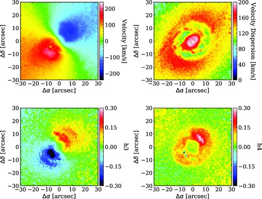
Stellar LOSVD moment maps of NGC 1097. Stellar velocity (top left-hand panel) velocity dispersion (top right-hand panel) Gauss-Hermite moments h3 (bottom left-hand panel) and h4 (bottom right-hand panel).
To define the centre of the galaxy, we first attempted to fit ellipses to the flux distribution by using the ellipse routine of iraf5 software, but we realized that the flux distribution of the galaxy is asymmetric, so the parameters of the ellipses were poorly constrained. Hence, we defined the photometric centre as the brightest spaxel in the nucleus based on the flux integrated over the entire MUSE spectral range. The kinematic centre derived in Section 3.3 differs only by ∼3 spaxels from thus defined photometric centre. Hereafter, we give the coordinates Δα, Δδ in relation to the photometric centre, i.e. the photometric centre is located at [Δα, Δδ] = [0,0].
2.2.2 Deriving ionized gas line-of-sight velocity distribution moments
We derived the ionized gas kinematics by fitting initially single Gaussian components to the emission lines, with the stellar continuum and absorption lines fitted simultaneously. The fits were performed on individual spaxels, while the stellar velocity moments were fixed to the values determined for each Voronoi bin, specified in the prior stellar kinematics fits. Computing Gauss-Hermite higher order moments is also possible for the emission line analysis, and we show the results of the fit including the h3 and h4 coefficients in Appendix A (Fig. A3). However, we find fitting emission lines with Gaussians to be a better approach when searching for multiple components (see Section 2.3), whose presence otherwise could be incorporated in the higher order moments.
DAP can fit each emission line separately or fit several emission lines together by assigning each the same velocity and velocity dispersion and by imposing flux ratios. We left the fluxes free, except for the constraints from atomic physics (Osterbrock & Ferland 2006). We gathered the emission lines into three main groups, with kinematics shared among lines in each group. Extracting kinematics for each group separately allows us to study and understand how gas regions of different physical properties move with respect to each other. The grouping of the emission lines is done as follows: Group 1 consists of Balmer lines – H βλ4861, H αλ6562 (indexed as H β and H α in figures); Group 2 consists of low-ionization lines – [N i]λλ5197,5200, [N ii]λ5754, [O i]λλ6300,64, [N ii]λλ6548,83, [S ii]λλ6717,31 and Group 3 consists of high-ionization lines – He iλ5875, [O iii]λλ4959,5007, [S iii]λ6312. We summarize the characteristics of the fitted emission lines in each group in Table 1.
Characteristics of the fitted emission lines. Wavelengths of the emission lines are taken from the National Institute of Standards and Technology (NIST; https://www.nist.gov/pml/atomic-spectra-database).
| Line ID | Wavelength | Amplitude ratio |
|---|---|---|
| (Å) | (fixed) | |
| Group 1 – Hydrogen Balmer Lines | ||
| H β | 4861.35 | – |
| H α | 6562.79 | – |
| Group 2 – Low ionization lines | ||
| [N i]λ5198 | 5197.90 | – |
| [N i]λ5200 | 5200.26 | – |
| [N ii]λ5754 | 5754.49 | – |
| [O i]λ6300 | 6300.30 | – |
| [O i]λ6364 | 6363.78 | 0.33[O i]λ6300 |
| [N ii]λ6548 | 6548.05 | 0.34[N ii]λ6583 |
| [N ii]λ6583 | 6583.45 | – |
| [S ii]λ6716 | 6716.44 | – |
| [S ii]λ6731 | 6730.82 | – |
| Group 3 – High ionization lines | ||
| [O iii]λ4959 | 4958.91 | 0.35[O iii]λ5007 |
| [O iii]λ5007 | 5006.84 | – |
| He i λ5876 | 5875.61 | – |
| [S iii]λ6312 | 6312.06 | – |
For each group, in Fig. 4, we present their kinematics accompanied by the flux maps of the strongest lines in each group, which are H α, [N ii]λ6583 and [O iii]λ5007, respectively. The flux maps of the weaker lines in each emission line group are presented in Fig. A.1. To avoid contribution from spaxels dominated by noise, we used a threshold SNR = 10; spaxels of lower SNR are discarded from the maps. All three groups show high flux in the nuclear ring and in the nucleus. The observed velocity field of each group has a typical spider velocity pattern and is dominated by rotation, but it also shows strong distortions from circular motion caused by the presence of the bar. Such distortions in the gas kinematics have been reported in various nearby galaxy studies (Bosma 1978; Emsellem et al. 2001; Fathi 2004; Zurita et al. 2004; Fathi et al. 2006). The velocity dispersion is the lowest in the nuclear ring and in the outer regions and significantly increases close to the nucleus.
![Flux and LOSVD moment maps of H α (left-hand panel) [N ii]λ6583 Å (middle), [O iii]λ5007Å (right-hand panel). We show the flux on logarithmic scale in units 10−20ergs−1cm−2spaxel−1 (top row) velocity (middle row) and the velocity dispersion (bottom row).](https://oup.silverchair-cdn.com/oup/backfile/Content_public/Journal/mnras/524/1/10.1093_mnras_stad1896/2/m_stad1896fig4.jpeg?Expires=1750260140&Signature=zEJ6P7zQHfJ8o7kscjt20LaFGpmu6L7eCmSs5OIS3LAH8VZ66L5sQ0KPKDSE8VcLZXdrbrpB474KBTa5AOLQPls6fGzrJnsOOSLdVmiIJrkEusoVg1S6qnfsem6R6vi5SnYUHWjqkiN~ilbFh7QSSqNn6QkGeMPBDBF0yaqUwoazsH~QlN47-aKgeBJDuF7ve9uXNNzg2WxLYnfPZRLlpp1NcH79AiJYxcN3trt1nYrPctn4TxYk5T6wJWODyriuz22GYhnWFc8huZCm0EuZC9zd~rIN74Bs4FdA3a40C4KZ~MSzFml0ob31Et~Wialt5CMkzCSOWP1FlEyjahxqZw__&Key-Pair-Id=APKAIE5G5CRDK6RD3PGA)
Flux and LOSVD moment maps of H α (left-hand panel) [N ii]λ6583 Å (middle), [O iii]λ5007Å (right-hand panel). We show the flux on logarithmic scale in units 10−20ergs−1cm−2spaxel−1 (top row) velocity (middle row) and the velocity dispersion (bottom row).
2.3 Improving the quality of the fits by fitting multiple Gaussians
In the regions inner to the nuclear ring, the kinematics of all emission line groups reveal a region of high velocity dispersion, extending from the centre of the galaxy ∼3 arcsec towards the north-east (see Fig. 4), which drove us to closely examine the spectra in the affected spaxels. In Fig. 5, we show the H α and [N ii]λλ6548,83 region of the spectrum in one of the affected spaxels, as well as in a spaxel outside of the affected region. These spaxels are located at the positions marked by an ‘x’ and a ‘+ ’, respectively, in the top left-hand panel of Fig. 6. In the spectrum of the affected spaxel, as shown in the middle panel of Fig. 5, we notice excess emission in the blue wing of [N ii]λ6583 line, with a peak at the rest frame wavelength ∼6574.50 Å, which hereafter we call the excess. Because of the excess, the line profile of [N ii]λ6583 becomes strongly non-Gaussian, and the excess encroaches on the region between [N ii]λ6583 and H α, so the H α fits are also strongly affected by its presence. As we demonstrate in the top panel of Fig. 5, when the excess is not present the emission lines are well-fitted, but when the excess is present the minimization algorithm of pPXF produces a broad Gaussian, especially for H α, leading to overestimated velocity dispersion values. The presence of the excess shifts the centre of the fitted Gaussians for the main [N ii]λ6583 component to slightly lower velocities, and for the H α component to higher velocities. We found no signs of an excess in the red wing of [N ii]λ6583, or either of the wings of H α. Although we see a weak excess in the blue wing of [N ii]λ6548, its SNR is at the same level as noise, and it is insignificant compared to the excess in the blue wing of [N ii]λ6583. Moreover, we found no signs of an excess in the wings of the [O iii]λ5007, though its presence might be lost to the noise. However, in the spaxels of the region with high velocity dispersion, where the presence of the excess in the blue wing of [N ii]λ6583 is the most pronounced, [O iii]λ5007 line is well-fitted. This suggests that the high velocity dispersion of [O iii]λ5007 in those regions (Fig. 4) is intrinsic.
![Representative spectra zoomed on the region of H α and [N ii]λ6583, and the best fits from pPXF/DAP. The lines represent the MUSE spectrum (black), the combined best fit of the stellar template and emission lines (red), the best fit of emission lines (green), and the difference between the spectrum and the combined best-fitting stellar template with emission lines (orange). top: Spectrum of a spaxel without the excess, marked in the upper left-hand panel of Fig. 6 with a ‘ + ’. middle: Spectrum of a spaxel with the excess affecting the single Gaussian fits of H α and [N ii]λ6583, marked in the upper left-hand panel of Fig. 6 with an ‘x’. bottom: Spectrum of the spaxel shown in the middle panel, with fits that include the secondary component.](https://oup.silverchair-cdn.com/oup/backfile/Content_public/Journal/mnras/524/1/10.1093_mnras_stad1896/2/m_stad1896fig5.jpeg?Expires=1750260140&Signature=cJpMsHVgM7a-0w8nq3CIGD7TdtjAaMTH~Z0CrvHeuTuilwqyunhAXjrdlfJ~qSAH-XJIFkZgQbnxJA41Ch8MjG5dz9WYEzeMc7TxyvKIfHOl34V~gjaJuuRHPiyFdSumLOzxe3V39~4R9JBKlwhTQaa0VYXWCSmUl-hcbFdsQoCl0F8TlMKTbaSHR6xiN~g1~XruzkTO97jEdqAxw5FupSETdvtTfv5aMuR92KcajErBw55HDs2zipKSWy2f2DfYSwirCvpXx2Sl2y0Gu2H2hmBdJaYALjYiltChLXzKYxuXPpkYUUVaUkPsuk5Zu8oHJ9twZy2ZSlLheGh9xr9W8Q__&Key-Pair-Id=APKAIE5G5CRDK6RD3PGA)
Representative spectra zoomed on the region of H α and [N ii]λ6583, and the best fits from pPXF/DAP. The lines represent the MUSE spectrum (black), the combined best fit of the stellar template and emission lines (red), the best fit of emission lines (green), and the difference between the spectrum and the combined best-fitting stellar template with emission lines (orange). top: Spectrum of a spaxel without the excess, marked in the upper left-hand panel of Fig. 6 with a ‘ + ’. middle: Spectrum of a spaxel with the excess affecting the single Gaussian fits of H α and [N ii]λ6583, marked in the upper left-hand panel of Fig. 6 with an ‘x’. bottom: Spectrum of the spaxel shown in the middle panel, with fits that include the secondary component.
![Comparison between fits using a single Gaussian and fits including a secondary [N ii]λ6583 component. Grey contours in all panels highlight the H α emission. The left-hand and right-hand columns represent H α and [N ii]λ6583, respectively. Top: the corrected velocity dispersion ‘x’ and ‘+’ markers on the left-hand panel represent the spaxels whose spectra are displayed in Fig. 5. middle: The ratio of velocity dispersion obtained from single Gaussian fits to the corrected velocity dispersion. Bottom: The velocity differences between the corrected velocity field and the velocity field obtained with single Gaussians.](https://oup.silverchair-cdn.com/oup/backfile/Content_public/Journal/mnras/524/1/10.1093_mnras_stad1896/2/m_stad1896fig6.jpeg?Expires=1750260140&Signature=lxOmScAkHKr5QpHfzpV9NG~mzGmIN1pxZT-YcdYi636Oy3oLnHDhdre3wqzaG4wyxfJPWudhnRgmmh49CVZuFld52vsbn8WJcbDGhcj1tiux1vO2-jamJMXLqi1cUbWrT8lOComYQoGU10ACC3zgSGp7EvxFmaW0JEIM~8bO2ruxfi~2ltPXmD0aEcmhznq4OGtgCFn6b9thvKyW~F7jIi44UjySNiKK8HpyPR9iVfI8xgLbfxhFi1QFLchFXA0pshH0d6wwJ4MzBFniu3Sz-j9xi~MRfjBvz45-N0fcuSUphOHvBCItcaVzAUPZBMsxT9IpybBPhDvIh~967X0FpQ__&Key-Pair-Id=APKAIE5G5CRDK6RD3PGA)
Comparison between fits using a single Gaussian and fits including a secondary [N ii]λ6583 component. Grey contours in all panels highlight the H α emission. The left-hand and right-hand columns represent H α and [N ii]λ6583, respectively. Top: the corrected velocity dispersion ‘x’ and ‘+’ markers on the left-hand panel represent the spaxels whose spectra are displayed in Fig. 5. middle: The ratio of velocity dispersion obtained from single Gaussian fits to the corrected velocity dispersion. Bottom: The velocity differences between the corrected velocity field and the velocity field obtained with single Gaussians.
In order to account for the excess and to improve the line fits, we introduced one additional emission component to the DAP configuration at wavelength λ ∼6574.50 Å, which we call the secondary component. Throughout the rest of this work, we work under the assumption that the secondary component is a Doppler-shifted component of [N ii]λ6583. We tested how the derived kinematics depends on the initial guess of the wavelength of the secondary component by shifting it by ±3.3 Å (roughly equal to the dispersion broadening); we find no significant changes to the results. In the bottom panel of Fig. 5, we demonstrate that for the spaxel, whose spectrum and single Gaussian fits were affected by the presence of the excess, the addition of the secondary component accounts for the excess, and fixes the erroneous fits. However, one must be careful, as for the spaxels where the excess is not strong the fits of the secondary component would be poorly constrained, and we must carefully determine the spaxels truly affected by the presence of the excess. This can be done by comparing the measurements extracted from fits with and without the secondary component. As we explained earlier in this section, the excess emission on one side of the line not only increases the velocity dispersion of a single Gaussian fit but also alters its velocity. While high velocity dispersion can be intrinsic, a large change in the derived velocity caused by including the secondary component indicates strong asymmetry of the line profile, hence, likely the presence of multiple line components. Therefore, we search for the spaxels that are most affected by the presence of the excess by looking for a change in derived velocities, which should be more reliable than using the high velocity dispersion measurements.
In order to identify which spaxels in and around the region of the elevated velocity dispersion in the nucleus are affected by the presence of the excess, we fitted the secondary component in the inner 8×8 arcsec2. In Fig. 6, we show the change in velocity (V) and velocity dispersion (σ) between the original values obtained from single Gaussian fits and the corrected values obtained from fits with the secondary component included. For the corrected measurements, in addition to the respective emission line ID, we use the notation ‘corr’.
The velocity dispersion in the nuclear regions remains high after including the secondary component (upper panels), with the values for [N ii]λ6583 and H α velocity dispersion reduced by ∼20–30 per cent and ∼30–40 per cent, respectively, from the values obtained from single Gaussian fits which might indicate the velocity dispersion is intrinsically high. The persisting high velocity dispersion might also suggest that our approach is simplistic and that using more than two Gaussian components possibly can account for the excess better and can reduce the estimated velocity dispersion more. However, increasing the number of components introduces more free parameters, and we do not have enough constraints or resolution to fit more than two components. Moreover, we notice that the largest reduction in velocity dispersion (middle panels) occurs in spaxels where adding the secondary component significantly changes the velocity of the main lines (lower panels).
Therefore, based on the bottom panels of Fig. 6 we defined the following conditions to create a mask region where single Gaussian fits are not reliable, and values from the run with the secondary component will be used:
V[N ii]λ6583 − V[N ii]λ6583, corr < −4 km s−1
VHα − VHα, corr > 5 km s−1
−6 arcsec ≤ Δα ≤ 1.2 arcsec and −3 arcsec ≤ Δδ ≤ 4 arcsec
The application of the conditions above is shown in the left-hand panel of Fig. 7. The spatial cuts are applied to discard the isolated spaxels outside the region of the elevated velocity dispersion in the nucleus where the velocity correction is low. The velocity limits are chosen to maximize the area where the secondary component can be reliably fitted. By replacing within the defined mask region, the measurements from the single Gaussian fits with those from fits with the secondary component included, we created a combined data set of corrected flux, velocity, and velocity dispersion. The resultant maps are presented in Fig. A2. For both H α and [N ii]λ6583, the apparent change in flux, velocity, and velocity dispersion maps are not significant. However, the accurate corrected values are crucial for our further analysis in Section 3. Hereafter, we use measurements from the combined data set. [O iii]λ5007can still be represented by the maps in Fig. 4 since single Gaussian fits were not affected by the presence of the excess.
![Left-hand panel: The mask of spaxels for which the fits including secondary component were used in further analysis. Spaxels in the grey-shaded region fall outside the defined conditions and are excluded from the mask. Blue and red colours, cut respectively at the 5 and 4 km s−1 thresholds, show the difference between velocities extracted by fitting single Gaussians and after including the secondary component for H α and [N ii]λ6583. Grey contours represent the H α emission. The centre of the galaxy is marked with a cross. Right-hand panel: Flux and kinematics of the secondary component within the mask. Only spaxels within the mask are shown. Maps respectively show the derived flux (top left-hand panel), velocity (top middle), velocity dispersion (top right-hand panel), the ratio of the fluxes of the secondary component and the main [N ii]λ6583 line (bottom left-hand panel), the difference in velocities of the secondary component and the main [N ii]λ6583 line (bottom middle), the ratio of velocity dispersion of the secondary component and the main [N ii]λ6583 line (bottom right-hand panel).](https://oup.silverchair-cdn.com/oup/backfile/Content_public/Journal/mnras/524/1/10.1093_mnras_stad1896/2/m_stad1896fig7.jpeg?Expires=1750260140&Signature=PlmYUcNgIur5rAM91FEhIB6buCm3Jd1Qev74WL~rs8dIQuPfzV5b86Qnc0m0EUQzb3WhXWTUgu-sM3vJE5Aq0sLPzspwYv8Ohr~rAcI1Qc8lmCczt01c5W6WF~yIDR0XfQ1PY8nHEfIkysB6sMNs0ckd19B3lC2f05zawEp0zgXwgd~5KNqu0PuIafNZIW8YybAf5z~RP7tByLeIuhL8W0Va9YnzyGw1AICesHB~fC1E9T4UE7OZtfcFAWE5xqZ9elVFXZREYROgj1iRqZRnuEvSUUZQva2t6I08Xschi-dskMrRBdeeTtxNcsBGeZiOMTCsFKto7lpSAa~mW1tIKA__&Key-Pair-Id=APKAIE5G5CRDK6RD3PGA)
Left-hand panel: The mask of spaxels for which the fits including secondary component were used in further analysis. Spaxels in the grey-shaded region fall outside the defined conditions and are excluded from the mask. Blue and red colours, cut respectively at the 5 and 4 km s−1 thresholds, show the difference between velocities extracted by fitting single Gaussians and after including the secondary component for H α and [N ii]λ6583. Grey contours represent the H α emission. The centre of the galaxy is marked with a cross. Right-hand panel: Flux and kinematics of the secondary component within the mask. Only spaxels within the mask are shown. Maps respectively show the derived flux (top left-hand panel), velocity (top middle), velocity dispersion (top right-hand panel), the ratio of the fluxes of the secondary component and the main [N ii]λ6583 line (bottom left-hand panel), the difference in velocities of the secondary component and the main [N ii]λ6583 line (bottom middle), the ratio of velocity dispersion of the secondary component and the main [N ii]λ6583 line (bottom right-hand panel).
We present the flux (F) and kinematic maps of the secondary component (indexed by [N ii]w) within the mask region in the right-hand panel of Fig. 7, both absolute and relative to the main [N ii]λ6583 component. Note that few spaxels within the mask show inconsistent values compared to the main gradient of flux and kinematic measurements. This implies that the secondary component fits in those spaxels are not reliable and those spaxels are discarded in the analysis below. The secondary component has high flux at the centre of the galaxy that extends towards the north-east side of the mask, coinciding with the high velocity dispersion of the H α and [N ii]λ6583 components. In addition, the flux ratio of the secondary component to the main component increases away from the centre. In the velocity map of the secondary component, we see a gradient consistent with rotation, but after we subtract the disc rotation, the secondary component appears blueshifted by 300–400 km s−1 with respect to the main component, and the blueshift decreases away from the galaxy centre. The velocity dispersions of the secondary and main components are similar, though there is a slight indication that in spaxels where the contribution from the secondary component is the strongest, its velocity dispersion is smaller than that of the main component by up to 20 per cent.
3 ANALYSIS OF THE DERIVED KINEMATICS AND FLUXES
3.1 Searching for coherent kinematic structures in deviations from circular motion
Coherent structures in velocity maps can be best traced when the rotational component of motion is removed from the data. It is most commonly done by subtracting the line-of-sight (LOS) velocity of a simple rotating disc from the observed LOS velocity. The result is displayed in a spatial map, which is called the residual velocity map. Coherent structures in the residual velocity map will indicate large-scale motions of gas that depart from circular trajectories. In particular, shocks in gas result in velocity discontinuities, and large-scale shocks are expected to appear as coherent structures in the residual velocity map.
In Fig. 8, we demonstrate what we define as coherent structures in a residual velocity map. In its upper panel, we present the LOS velocity of a representative thin flat rotating disc which we constructed using Kinemetry software (Krajnović et al. 2006), described in detail later in this section. The disc orientation parameters, position angle (PA) of the line of nodes (LON) of 137°, and inclination (i) of 35°, are taken from the literature (Fathi et al. 2006). In the bottom panel of Fig. 8, we present the constructed residual velocity map after subtracting the LOS velocity of the modelled disc from the observed H α velocity. The residual velocity map reveals two straight continuous structures, one with positive and one with negative residual velocities, which are roughly parallel to the LON and are offset from the LON to the top left and bottom right. Such large residual velocities appearing over continuous stretches in the velocity map are associated with bar-induced shocks in gas which cause velocity jumps. The shocked gas loses angular momentum and funnels from the outer regions of the galaxy towards the inner regions. As shocks compress the gas, which is well mixed with dust, they also coincide with the loci of the dust lanes. Therefore the alignment of the kinematic structures with large residual velocities shown in Fig. 8 and the dust lanes shown in Fig. 1 signifies the presence of large-scale shocks that extend from the outer regions of the bar towards the central regions. Although gas inflow in bar-induced shocks is efficient, in Fig. 8 it can be seen that the straight shocks weaken in the central regions. As the result, inflow slows down, and the density of the gas increases which can trigger SF and form stellar substructures like the nuclear rings (Shlosman et al. 1989; Athanassoula 1992; Martini et al. 2003; Kim et al. 2012). This effect is seen in the central ∼8 arcsec of NGC 1097, where the stretches of large residual velocities are connecting to the nuclear ring (shown in Fig. 8). The continuous accretion of material along the bar onto the nuclear ring plays a crucial role in regulating SF activities (Sormani et al. 2023).
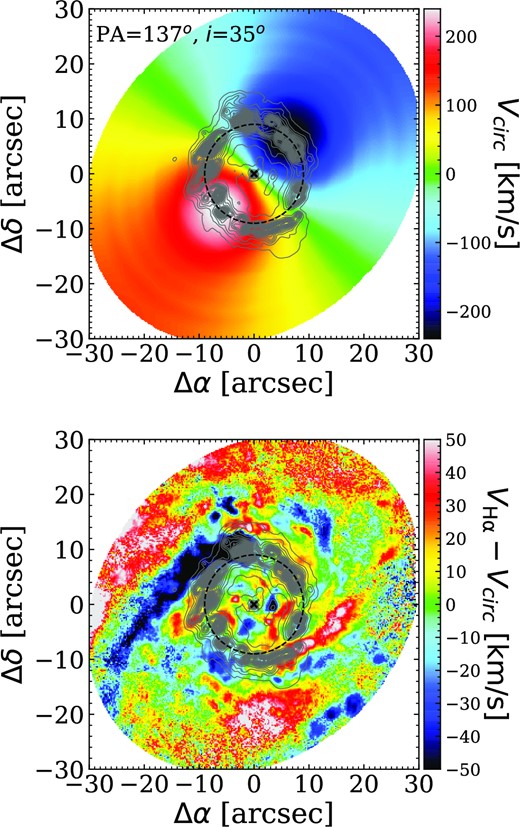
Top: LOS velocity of the rotating disc fitted to observed H α velocity field with PA of the LON = 137° and i = 35°. Bottom: Residual velocities after subtracting the LOS velocity of the modelled disc from the observed H α velocity. Grey contours highlight the H α emission. The nuclear ring is represented by the black dashed circle. The centre of the galaxy is marked with a cross.
Thus, although we have a good understanding of the bar driven gas inflows to the central regions, we lack an understanding of the inflow to the innermost nuclear regions. In this work, we aim to identify the inflow of gas from the nuclear ring towards the nucleus of the galaxy by searching for coherent structures in the residual velocity fields. Since subtracting the LOS velocity of an incorrectly fitted disc from the observed velocity will obscure the real features (van der Kruit & Allen 1978), we need to construct the most accurate disc model. To do this, we must cautiously determine the galaxy centre and disc orientation parameters: PA of the LON and i. Below, we explain in detail the procedures of constructing a flat disc in circular motion. For a flat thin disc in circular motion, the distribution of LOS velocities can be expressed by:
where Vsys and VC are the systemic and circular velocity, respectively, i and ψ are the inclination of the disc and azimuthal angle measured counterclockwise from the LON in the galaxy plane, and R is the radius of a circular ring in the galaxy plane. Inclination is directly related to the flattening parameter (or axial ratio) q (cos(i) = q) of the disc projected on the sky, which is an ellipse with major axis on the LON and ellipticity ϵ = 1 − q.
To determine the orientation of the rotating disc model, we employed Kinemetry, which is software specifically designed for IFU data and is a generalization of surface photometry to higher order moments of the LOSVD (Krajnović et al. 2006). Kinemetry performs harmonic expansion along best-fitting ellipses of the optimal major axis’ PA, optimal ellipticity, and centre using Fourier analysis. When applied to the velocity field, it produces the distribution of velocity along ellipses of semimajor axis a, K(a,ψ), described by a finite number of harmonic terms:
where ψ is the eccentric anomaly, equivalent to that in equation (1). To determine the best-fitting ellipse, the appropriate harmonic terms are minimized. Under the assumption of emission from a thin disc structure and fixed centre, Kinemetry reduces to the tilted-rings method, which breaks the disc into individual rings with different i, PA of the LON and rotational velocity (Rogstad, Lockhart & Wright 1974).
Since we want to fit the rotating disc to the gas motions, we use the H α velocity field as the input for Kinemetry. To ensure the thin flat rotating disc is accurately fitted we performed three Kinemetry fits, starting from one with all orientation parameters allowed to vary and gradually fixing the global orientation parameters in the consecutive fits. In Fig. 9, we summarize the estimated parameter distributions from each fit. In determining the global values for the disc orientation parameters, we discard parameters estimated within the inner 2 arcsec as the estimations within this radius are unreliable because of the insufficient data that ellipses are being fitted to, and because of the impact of the AGN.
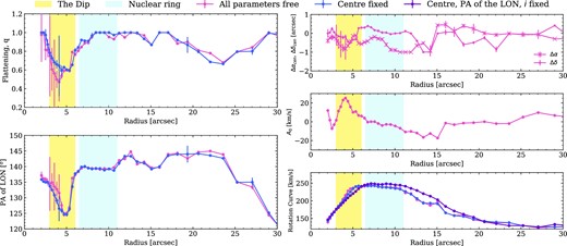
Radial distributions of parameters fitted to the H α velocity field with Kinemetry. The blue-shaded region represents the nuclear ring and the yellow-shaded region marks the radial range where PA of the LON and i vary significantly (the Dip). Results from the run with all parameters in the Kinemetry fit allowed to vary freely are shown in pink, results for the centre and A0 fixed are shown in blue, and results for the PA of the LON, i, centre, and A0 fixed are shown in purple. The left-hand panels display the flattening, q (top) and the PA of the LON (bottom). The right-hand panels show the coordinates of the kinematic centre (top), the A0 coefficient (middle), and the rotation curve (bottom).
We first fitted the velocity field by allowing the orientation parameters of each ellipse, including the centre, to vary freely. As shown in the top right-hand panel of Fig. 9, in the regions inward from the nuclear ring, the horizontal (Δα) and vertical coordinates (Δδ) of the kinematic centre show only small variations (∼0.7 arcsec for Δ α and ∼0.5 arcsec for Δδ) from the photometric centre. This indicates that in the regions inner to the nuclear ring, the estimated kinematic centre agrees with the photometric centre within ∼3 spaxels. Also, as shown in the middle right-hand panel of Fig. 9, the A0 values for ellipses fitted interior to the nuclear ring depart from the systemic velocity of the galaxy by less than 25 km s−1. Therefore, we reduced the number of free parameters within Kinemetry by fixing the centre of the galaxy to the coordinates of the photometric centre, and the A0 to the velocity at the photometric centre (−3.55 km s−1), and performed a second fit. In this second fit, we intended to estimate a representative PA of the LON and i which can accurately describe the ellipses in nuclear regions, and we aimed to build our final circular disc model by fixing the PA of the LON and i to these estimated representative values. However, as shown in the left-hand panels of Fig. 9, regardless of keeping the centre free or fixed, in the regions inward from the nuclear ring, the distributions of the PA of the LON and i strongly fluctuate within a radial region marked in yellow, which we refer to as the Dip. Within the Dip, the PA of the LON from the second fit varies between 125° and 140°, and q varies between 0.65 and 0.90, which translates to an i range of ∼25°– 48°. While the impact of bar-induced non-circular motions can justify the fluctuation of these parameter values outside the nuclear ring, inward from the nuclear ring one would expect motion close to circular and therefore well fitted by single values for the PA of the LON and i. However, this expectation might be simplistic, as NGC 1097 is proposed to be hosting a nuclear bar (Buta & Crocker 1993; Shaw et al. 1993) which would impact the gas flow in the regions inward from the nuclear ring.
As we indicate above, in the third Kinemetry fit we want to fix the PA of the LON and i to fit a flat disc, but it is challenging to deduce reliable parameter values from such fluctuating distributions. Moreover, in Fig. 8, which presents residual velocities for a thin disc fit with parameters taken from the literature (PA of the LON = 137° and i = 35°; Fathi et al. 2006), in the region inner to the nuclear ring we notice a periodic azimuthal variation resembling an m = 3 mode. Our initial explanation for it was that i used in the disc model was higher than the true value, which would give artefacts in the residuals in the form of m = 3 harmonic terms (van der Kruit & Allen 1978; Franx, van Gorkom & de Zeeuw 1994; Schoenmakers, Franx & de Zeeuw 1997). Artefacts can be removed by choosing an i value in the disc model that is closer to the actual i of the galaxy, but variations in Kinemetry parameters are preventing us from settling on a reliable i.
Therefore, to find the i value for which the residuals of the Kinemetry fits are free from the m = 3 azimuthal variations, we investigated the effect of changing the i and PA of the LON on residual velocities by running Kinemetry first with a fixed PA of the LON at 137° and different q (0.7, 0.9), and then with a fixed q at 0.82 (i ≈35°) and different PA of the LON (125°, 140°). We constructed the corresponding residual velocity maps and examined the residuals, as we show in Fig. 10, to deduce which parameter set is best for the final disc model. When the disc is modelled with the PA of the LON 125° and i 35°, we see the m = 1 harmonic terms in the residual velocity map as an effect of wrongly fitted PA of the LON, with one side of the map having mainly positive velocities and the other side having mainly negative velocities (van der Kruit & Allen 1978). However, these artefacts can be largely eliminated by adopting the optimal PA of the LON. We also see m = 3 harmonic terms in all panels. They are strongest in the bottom right-hand panel where we notice both positive and negative residual velocity regions extending radially from the centre beyond the nuclear ring. We must emphasize that no matter what inclination is used in the disc model, m = 3 azimuthal variation in the residual velocity is only minimized and not eliminated. The i within the range of 25°– 35° minimizes its amplitude, yet we do not see a clear minimum.
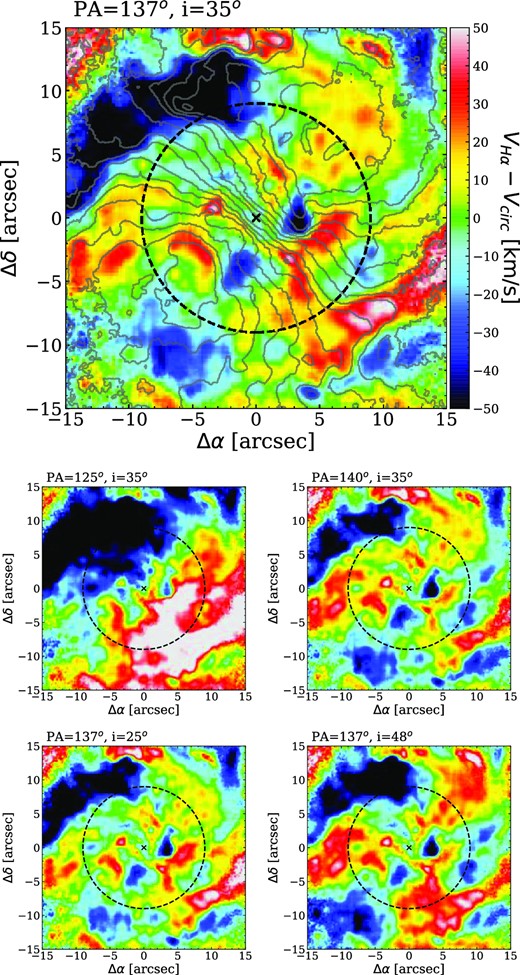
Residual velocity map of the inner 30×30 arcsec2. The dashed circle represents the nuclear ring. The centre of the galaxy is marked with a cross. In each panel, we subtract the LOS velocity of the disc modelled with a different combination of PA of the LON and i. top: PA = 137° and i = 35° (q = 0.82) as in Fig. 8. The grey contours represent the H α velocity field. middle: i is fixed at 35° and PA of the LON is varied. bottom: PA of the LON is fixed at 137° and i is varied.
The range of acceptable parameter values agrees well with the parameters in the literature: the kinematic position angle, PA = 135°, derived in Storchi-Bergmann et al. (1996) and Emsellem et al. (2001); inclination, i = 34°, derived in Storchi-Bergmann et al. (2003) for the nuclear accretion disc, and i = 35° derived in Fathi et al. (2006) from exponential thin disc model. Therefore we conclude that the disc parameters, PA = 137° and i = 35°, taken from Fathi et al. (2006) and applied in Fig. 8, are optimal. Although the parameters, PA = 122° and i = 48° adopted by Lang et al. (2020) differ from our optimal parameters, we show in Fig. 10 that each of these parameters would give artefacts in the residual velocity.
Due to the smoother nature of the stellar velocity field compared to the gas velocity field, it is generally expected to obtain more continuous parameter distributions when fitting a disc to the stellar velocity field. However, the large velocity dispersion inward from the nuclear ring of NGC 1097 (Fig. 3) reduces the LOS velocity values over an elliptical region inconsistent with a projected disc in an acceptable inclination range, and therefore is likely to result in an incorrect fit, which we indeed observed when using Kinemetry. Therefore, parameters estimated by fitting the stellar velocity field would not be reliable inward from the nuclear ring. On the other hand, the PA of the LON and i that we derive with Kinemetry for the stellar velocity field outside the nuclear ring is consistent with our adopted values, although the PA of the LON diverges at larger radii, likely because of the influence of the bar. Furthermore, disc orientation parameters cannot be reliably obtained from large-scale photometry due to the presence of companion and asymmetric spiral arms.
Since, even for the optimal parameters, a flat disc in circular motion does not provide a good fit to the data, because periodic azimuthal variations of residual velocities persist in those regions, we revisited the LOS velocity fields of each emission line group to check if there are any signs of these features directly in the observed velocity fields. In the top panel of Fig. 10, we superimpose H α velocity contours on the residual velocity map to show that in the regions inward from the nuclear ring, the H α velocity field shows wiggles at loci coinciding with two most prominent negative residual velocity regions that we interpreted above as part of the m = 3 harmonic terms. This indicates that the features which we initially interpreted as artefacts of the fit arise from real features present in the data. Hence, in Section 3.2, we focus on examining the physical processes in the regions inner to the nuclear ring, which may give rise to some of the kinematic structures observed in the velocity map.
3.2 Dominating ionization mechanisms in the centre of NGC 1097
To determine the dominating source of ionization from optical emission lines, such as AGN or star-forming regions, one can use the Baldwin, Phillips & Terlevich (BPT) diagram (Baldwin, Phillips & Terlevich 1981). In the left-hand panel of Fig. 11, we show the BPT diagram for the inner 30 ×30 arcsec region of NGC 1097. Each point on the diagram corresponds to a spaxel in the data, with its position determined by the fluxes measured for that spaxel. We mask spaxels with poor flux measurements by applying an amplitude-over-noise (AON) ratio (Sarzi et al. 2006) threshold of 7, which excludes spaxels with AON≤7 from the BPT diagram, choosing a smaller threshold would give noisy results already occurring outside the nuclear ring in Fig. 11. This allows us to focus on the emission that is coming from the nuclear ring and the region inner to it. To distinguish AGN from star-forming regions, we used the Kewley et al. (2001) (hereafter Kewley+01) relation which indicates what line ratios can be produced by stellar photoionization, as points above the Kewley+01 line likely originate from the AGN activity or shocks. However, the Kewley+01 relation does not take into account the composite emission which has a contribution from SF, hot old low-mass stars and AGN. Therefore, to include the composite emission, we used the modified Kewley+01 line from Kauffmann et al. (2003) (hereafter Kauffmann+03) so that the region between Kauffmann+03 and Kewley+01 lines is the location of the composite sources, and points below the Kauffmann+03 line indicate emission purely coming from SF. We also separated the AGN region into two classes, LINER and Seyfert region, based on the relation given by Cid Fernandes et al. (2011).
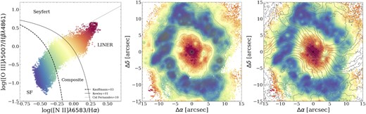
Left-hand panel: The BPT diagram of the inner 30×30 arcsec2 region. The SNR = 10 and AON = 7 thresholds are applied. Each point represents one spaxel. The dashed, solid, and dotted lines represent the Kauffmann et al. (2003), Kewley et al. (2006), and Cid Fernandes et al. (2011) fits, respectively, which establish the dominating ionization mechanisms. The colour coding is based on the distance from the Kewley et al. (2006) line. Middle and right-hand panel: Maps of the inner 30×30 arcsec2, with colour coding of the spaxels taken from the left-hand panel. Contours represent H α flux (middle) and LOS H α velocity (right-hand panel).
Each point in the BPT diagram represents a spaxel and is colour coded according to its distance from the Kewley+01 line. This colour coding is then used in the spatial map to highlight which sources of ionization dominate in what regions (Fig. 11 central and right-hand panels). We also included H α flux and velocity contours on the spatial maps to combine the BPT diagram results with kinematics and light distribution.
In the nuclear ring, the emission is strongly dominated by SF, while the regions inward from the nuclear ring predominantly show LINER emission. However, three locations in the regions inward from the nuclear ring (∼5 arcsec east and west and ∼2 arcsec north-west from the centre) show composite emission due to contribution from SF and have high H α flux (see also Fig. 4). The region of composite emission to the west has the highest contribution from SF (is closest to the Kauffmann+03 line in the BPT diagram) and it appears to be part of a structure with elevated SF that extends from the nuclear ring directly north of it towards a smaller region of the composite emission to the south. The H α velocity field throughout the extent of this structure is strongly disturbed (Fig. 11 right-hand panel), which can be caused by stellar outflows associated with elevated SF. Moreover, this structure also coincides with the strong negative velocity residual (Fig. 10), suggesting that the negative velocity residuals, which we initially interpreted as artefacts caused by adopting the wrong inclination of the fitted disc, arise from real features present in the data. The region of composite emission to the east shows a weaker SF component than the region to the west. This region is also associated with a disturbed H α velocity field, and unlike the region to the west which is extended tangentially in the North–South direction, it is curved towards the nucleus of the galaxy. Lastly, the region of the composite emission to the north-west has the weakest contribution from SF, and the H α velocity field in that region is only mildly disturbed. Compared to the other two regions, this region appears to be more isolated yet it still clearly shows in the velocity residuals in Fig. 10.
3.3 Searching for coherent kinematic differences between distinct emission line groups
We showed in Section 3.1 that velocity residuals after subtracting a flat disc in circular motion do not provide conclusive information about coherent kinematic structures inner to the nuclear ring. Here, we explore what kinematic information can be extracted from the data without relying on kinematic or mass models. In Fig. 12, we compare the LOSVD moments of the Balmer and low ionization lines by constructing the maps of [N ii]λ6583/Hα line flux ratio (left-hand panel), velocity difference (middle panel) and velocity dispersion ratio (right-hand panel).
![Left-hand panel: Line flux ratio of [N ii]λ6583 and H α. Middle: The velocity difference map, which is constructed by subtracting the LOS velocity of H α from the LOS velocity of [N ii]λ6583. Black contour marks the region where the velocity difference between [N II]λ6583 and H α was more than 30 km s−1 for single Gaussian fits. Right-hand panel: Velocity dispersion ratio of [N ii]λ6583 and H α. In all panels, grey contours highlight the H α emission.](https://oup.silverchair-cdn.com/oup/backfile/Content_public/Journal/mnras/524/1/10.1093_mnras_stad1896/2/m_stad1896fig12.jpeg?Expires=1750260140&Signature=3fgnIGASwVexPrFvLta5GsvO9GBQqe~hl6dkpnJZsaj94QVKn0zjq4KNsvcx~rlPEtmtumk4zjAE3JqeqmRz9nENPENWVPWRNADy6fXm3HWqEKCVFgvrqx7yQ6twdPH4IFqBoij59jZDebGPfFJXZyulIkXvI45XDh6jsa2Q7p2bTJBIeWdraV2gxiiq7YHFfdZdHnLC1AD0v5XTyK1kpSrWqkgOpt2lAQLAkL6zRfa~t7FB3A7J39w0Tj2En0r2p12Rw0QZVX5MBPQ6Elwdk7uEe8DFUHkgi7WmduBUw~9qJKXAOXfrOkG9XbqIBachFCKciTRvcDAb0kuPUCjYxQ__&Key-Pair-Id=APKAIE5G5CRDK6RD3PGA)
Left-hand panel: Line flux ratio of [N ii]λ6583 and H α. Middle: The velocity difference map, which is constructed by subtracting the LOS velocity of H α from the LOS velocity of [N ii]λ6583. Black contour marks the region where the velocity difference between [N II]λ6583 and H α was more than 30 km s−1 for single Gaussian fits. Right-hand panel: Velocity dispersion ratio of [N ii]λ6583 and H α. In all panels, grey contours highlight the H α emission.
[N ii]λ6583 emission, with higher ionization potential, may predominantly originate from post-shock gas, while Hαemission, mostly generated by stellar photoionization, is less affected by the shock. Therefore, in the regions where shocks are present, the observed [N ii]λ6583/H α line flux ratios should be elevated. As shown in the left panel of Fig. 12, [N II]λ6583/Hαis the lowest in the nuclear ring where SF dominates the emission, and it is the highest in the nucleus where the AGN dominates. There are no other regions inward from the nuclear ring with elevated [N ii]λ6583 emission. Instead, we notice regions of elevated H α flux associated with enhanced SF (see Section 3.2), which might be obscuring the possible enhancement in [N ii]λ6583 in the same region if SF is triggered by shocks. Nevertheless, if [N II]λ6583 around shocks originates mostly from the post-shock gas, large-scale shocks can manifest themselves by velocity differences between [N ii]λ6583 and H α that are coherent over large distances, as explained below. The velocity of each tracer evaluated in a spaxel is the first moment of the LOSVD arising from integrating the emission along the LOS and over the spaxel area. If this includes regions of gas with different physical conditions which move with respect to each other, the integrated LOSVD recorded in a spaxel should vary between the tracers, as relative contributions to line emission from regions with different physical conditions differ between emission lines. Consequently, the value of its first moment may differ for each tracer.
A good example of two neighbouring gas regions that differ in physical conditions and move with respect to one another are regions upstream and downstream from a shock in gas. Commonly temperature and pressure are higher in the post-shock gas than in gas upstream from the shock, and jump conditions in the shock impose a velocity difference between these two regions. Hence, for a spaxel which records emission from pre-shock and post-shock regions, the derived [N ii]λ6583 and H α velocities will differ, as the former will be more representative of the post-shock region. Then, if large-scale shocks are present, they will appear as continuous structures in the velocity difference map, in which the velocity difference takes consistently positive (or negative) values. In the velocity difference map shown in the middle panel of Fig. 12, we notice a coherent blue feature of negative velocity difference spiralling out from the nucleus towards the south-east side of the nuclear ring, hereafter called the blue spiral arm. If it is a signature of shock in gas, it may be a spiral shock (Maciejewski 2004) extending inwards from the large-scale straight shocks in the bar of NGC 1097 (Fathi et al. 2006). The largest velocity difference in the blue spiral occurs at the location where the blue spiral curves towards the nucleus and is cospatial with the Hαenhancement to the east and with enhanced SF (see Fig. 11). This may indicate that the enhanced SF is associated with the inner part of the spiral shock.
Furthermore, shock conditions give rise to random motions, which increase the velocity dispersion of [N ii]λ6583 in the post-shock regions. This can possibly be seen in the south-east region of the blue spiral arm, where the velocity dispersion of [N ii]λ6583 is higher than H α but in the region where the blue spiral curves towards the nucleus, the velocity dispersion of [N ii]λ6583 is only slightly above ∼1. In the region ∼5 arcsec west from the nucleus we notice the largest velocity dispersion ratio, which is cospatial with the largest velocity differences to the west, and the elevated [N ii]λ6583/H α line flux ratios in the same region, as well as the enhanced SF (Section 3.2), but this feature is less spatially coherent than the blue spiral arm.
Although the observed velocity differences between emission lines could result from obscuration, H α and [N ii]λ6583 emission wavelengths differ only by 20 Å, so differential extinction is negligible. While incorrect line fitting can also cause the difference in the derived velocities between tracers, we minimize that possibility by addressing the non-Gaussianity of the emission lines by including the secondary component of [N ii]λ6583 line in spaxels where the excess emission was present, as we explain in Section 2.3. In fact, fitting emission lines with single Gaussian components resulted in the largest velocity difference between Hαand [N ii]λ6583 in spaxels where the excess in the spectra was present. In the middle panel of Fig. 12, we mark with a black contour the region where the velocity difference ranged from −30 to −50 km s−1 for single Gaussian fits. Including the secondary component reduced this difference to ∼10 km s−1. The spectra throughout the blue spiral arm, which is outside the contour region, are well-fitted with single Gaussians, which indicates that the velocity difference between emission lines in those regions is not caused by the incorrect fitting.
4 DISCUSSION
4.1 Elliptical flow pattern in regions inward from the nuclear ring
We based our studies of residual velocities (Section 3.1) on the assumption that inward from the nuclear ring the flow of unperturbed gas is circular. However, we showed that in this region Kinemetry cannot accurately constrain the parameters of the unperturbed circular motion in a thin flat disc. The possible reason for this is that the unperturbed flow is either not flat or not circular there. In order to obtain meaningful residuals, one needs to first correctly identify the underlying flow.
If the flow is intrinsically circular, the PA of the LON and PA of the zero velocity line are perpendicular, but this is not the case if the global flow is intrinsically not circular (e.g. elliptical; see the appendix of Mazzalay et al. 2014). Here, we test whether in the regions inward from the nuclear ring the underlying flow is intrinsically non-circular, by determining the angle between the LON and the zero velocity line, where the distribution of the PA of the LON is inferred from Kinemetry.
In order to derive the distribution of the PA of the zero velocity line, for each column of spaxels in the velocity field (corresponding to constant Right Ascension), we identified the spaxel with the velocity closest to the systemic velocity of the galaxy. We then connected these spaxels to produce the fit of the zero velocity line. Further, we determined the PA of each spaxel on the zero velocity line which gives us the distribution of the PA of the zero velocity line with radius. We applied these steps on both stellar and H α velocity fields. We expect that the angle between the LON and the zero velocity line will be less affected by non-circular motion for stars than for gas because high velocity dispersion in stars hides the underlying non-circularity.
In the left-hand panels of Fig. 13, we show the H α and stellar LOS velocity maps and the corresponding zero velocity line fitted on each map. In the right-hand panel, we present the individual distributions of the PA of the LON and the PA of the zero velocity line for both velocity fields. In the figure, we show the PA of the zero velocity line values after subtracting 90°, which should be equal to the PA of the LON for circular motion. The distributions of the PA of the LON and PA of the zero velocity line for stars roughly align with each other over the whole radial range, differing slightly inside the Dip (see Section 3.1) by at most ∼5°. The values of the PA of the LON and PA of the zero velocity line for H α velocity field roughly converge in the nuclear ring, but within the Dip, the two differ by ∼15°–20°. This implies that in the regions inward from the nuclear ring, the underlying orbits of the gas flow are intrinsically non-circular, which prevents Kinemetry from accurately constraining the disc orientation.
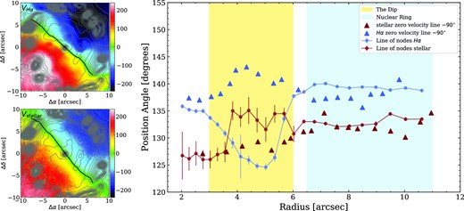
Left-hand panel: H α (top) and stellar (bottom) LOS velocity maps. The black line represents the corresponding zero velocity line fit. Grey contours represent the H α emission. The centre of the galaxy is marked with a cross. Right-hand panel: Distributions of the PA of the LON obtained from Kinemetry and PA of the zero velocity line. For the stars the distribution of the PA of the LON is plotted in small red circles and the PA of the zero velocity line in red triangles. For gas, the PA of the LON is plotted in small blue circles and the PA of the zero velocity line in blue triangles. The blue-shaded region represents the nuclear ring, and the yellow-shaded region represents the Dip defined in Section 3.1.
Thus, assuming an intrinsically circular flow of gas may compromise the search for coherent kinematic structures in the velocity residuals, and an oval or elliptical flow can be a better representation of the gas flow. Such assumption of an oval flow is allowed by the DiskFit software (Spekkens & Sellwood 2007), which is specifically developed for bar-like and oval distortions and allows fitting non-axisymmetric flow patterns to two-dimensional velocity fields. Although exploring this approach is plausible, it is outside the scope of this work.
4.2 Evidence from the MUSE data for nuclear spiral shocks
Studying the near-infrared images from the adaptive optics assisted NACO camera/spectrograph of the VLT, Prieto et al. (2005) found dust extinction in the form of a complex three-arm filamentary structure in the regions inner to the nuclear ring. The spiral arms of this structure are reaching to the centre from the north, south and west. Moreover, in good agreement with Prieto et al. (2005), a similar three-arm network is observed in the images from the Advanced Camera for Surveys (ACS) of the HST (Fathi et al. 2006). Hereafter we call this structure the nuclear dust filaments. In Fig. 14, we show the NACO image of Prieto et al. (2005). Inside the oval area, the image displays the residuals after subtracting the light profile of a simple ellipse model. In the figure, we include a dashed line to represent the proposed nuclear bar of the galaxy (Buta & Crocker 1993; Shaw et al. 1993), with a major axis PA of 28° (Quillen et al. 1995). We notice that the northern and southern arms of the nuclear dust filaments are roughly parallel to this nuclear bar, which is consistent with the expected geometry of dust lanes in a bar when the dust lanes are associated with gas inflow in shocks. The arm to the west of the nucleus is not readily associated with the nuclear bar.
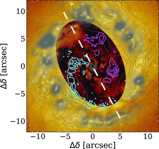
NACO J-band image from Prieto et al. (2005) with the light profile of a simple ellipse model subtracted inside the oval. The white dashed line represents the proposed nuclear bar with PA = 28° and length ≈ 20 arcsec (Quillen et al. 1995). Blue and pink contours represent the blue and red spiral arms in the velocity difference map (Fig. 12). Grey contours represent the H α emission.
In Fig. 14, in blue contours, we outline the blue spiral arm extending from the inner south-east part of the nuclear ring towards the nucleus which is revealed in the velocity difference map (Fig. 12, middle panel). The region of the blue spiral where it curves towards the nucleus is cospatial with the region of the composite emission directly to the east of the nucleus, which is associated with enhanced SF, and with the disturbed H α velocity field (Fig. 11). If the velocity difference is caused by the shock, as we argued in Section 3.3, then the blue spiral arm can be a nuclear spiral shock in which gas inflow to the nucleus occurs. For bisymmetric mass distribution, such shock should have a symmetric red component on the other side of the nucleus (Canzian 1993; Schoenmakers et al. 1997) in the velocity difference map. In Fig. 12, middle panel, we notice a red structure at ∼5 arcsec west of the nucleus extending from the nuclear ring towards the south, outlined in pink in Fig. 14. This structure is not curved towards the nucleus and does not have as defined spiral continuity as the blue spiral arm, but it has the highest velocity differences, it is cospatial with the region of the composite emission to the west, which has the highest contribution from SF, and it coincides with the strongest distortions of the H α velocity field. Hereafter, we call this structure the red spiral arm. We hypothesize that in the red spiral arm the gas density is higher compared to the region to the east, which leads to higher SF there, whose consequences, particularly outflows, dominate the shock signature there, while the SF is less dominant in the blue spiral.
The blue and red spiral arms are shifted ∼2–3 arcsec downstream from the northern and southern arms of the nuclear dust filaments. Hence, the combination of the structures observed in kinematics and morphology might be the imprint of the gas flowing to the nucleus under forcing from the nuclear bar. However, it is unclear whether the kinematic arms are directly associated with the dust filaments.
Hydrodynamical and kinematic modelling (Davies et al. 2009; Fathi et al. 2013) support a net molecular gas inflow to the nucleus, channelled via the arms of the nuclear dust filaments of Prieto et al. (2005). Using data from the Gemini Multi-Object Spectrograph (GMOS) on Gemini South Telescope, Fathi et al. (2006) studied the [N ii]λ6583 kinematics within the inner 15 ×7 arcsec2 region of NGC 1097, and revealed a three-arm spiral network in residual velocities centred on the galaxy nucleus with velocity amplitudes reaching |$\sim 20~{{\ \rm per\ cent}}$| of the rotational velocity, consistent with the nuclear spiral models of Maciejewski (2004). Moreover, Davies et al. (2009) studied the H2 kinematics within the inner 4 ×4 arcsec2 region and could resolve a two-arm kinematic spiral structure in their residual velocities. Benefiting from the large FoV of MUSE, we can trace these observed kinematic structures in our residual velocity map beyond their spatial coverage. We do not find any correlation between the structures found in the residual velocities by Davies et al. (2009) and our results, but the FoV of SINFONI is much smaller than the region to which we fitted the disc – Note that the SINFONI data have higher spatial resolution than the MUSE data, which might possibly make it harder to find a match as well.
Since Fathi et al. (2006) used [N ii]λ6583 data in their analysis, to compare our findings, we fitted our disc model with fixed PA of the LON = 137° and i = 35° (see Section 3.1) to [N ii]λ6583 velocity field. The resulting residual velocity map is presented in Fig. 15, which also includes the proposed three-arm kinematic spiral of Fathi et al. (2006). We do not find a coherent spiral network extending from the galaxy nucleus towards outer radii. Arguably, the proposed arm of the kinematic spiral to the south appears connected with a coherent structure in our residual velocity map, which might be extending from the nuclear ring towards the nuclear regions, but instead of curving towards the nucleus, it continues to the north-east. As already seen in Fathi et al. (2006) this arm runs along the arm of the nuclear dust filaments to the west. Hence, although in the region inward from the nuclear ring a three-arm spiral network is present in morphology (Prieto et al. 2005; Fathi et al. 2006), we do not find evidence of a spiral network in the residual velocities of the ionized gas. As we explained in Sections 3.1, 3.2, and 4.1, the data inward from the nuclear ring do not allow an accurate fit of a flat disc in circular motion, therefore residual velocities have to be interpreted with caution. On the other hand, in this work we find indications of nuclear spiral shocks in velocity difference maps.
![Residual velocities after subtracting the LOS velocity of the disc model from the observed [N II]λ6583 velocity field. The black dotted lines represent the kinematic spiral network of Fathi et al. (2006). The black dashed circle represents the nuclear ring. The centre of the galaxy is marked with a cross.](https://oup.silverchair-cdn.com/oup/backfile/Content_public/Journal/mnras/524/1/10.1093_mnras_stad1896/2/m_stad1896fig15.jpeg?Expires=1750260140&Signature=KvzVjr0JEH34wIaLYH0pIksjQHgjTdaMvalh5bwxixY99kvZvA877jtO5uOf~jwGSMLErD-vq8arAHiW9a6m23Q9Qr4Ge-LBljienTIY1YnimGqeUu~BgVS0w2~Yah9unuWXG1pcYUKzKvK5kGVs7EKVWtrJHagjNo2pWAtPxthir0Nr8hM8xne9gxZQS9v3bTj9PjjPu70njL04HfLCDxKrjhB6MhiaHs6UoG8qKm2fNIST4cHacW1EkEs8~fM5~pedFEgzgbpYRZAECVqcoBS0VQ1~HdOVrtwqQ8kvJ5oFhmJAUY4vRa4R24lYV0EnfAA2guGcpe2SgJy4uAbtKQ__&Key-Pair-Id=APKAIE5G5CRDK6RD3PGA)
Residual velocities after subtracting the LOS velocity of the disc model from the observed [N II]λ6583 velocity field. The black dotted lines represent the kinematic spiral network of Fathi et al. (2006). The black dashed circle represents the nuclear ring. The centre of the galaxy is marked with a cross.
4.3 Multiphase AGN outflows in the nuclear regions
As confirmed by a number of studies, the gas funnelling into the nucleus of NGC 1097 feeds its LINER core (Davies et al. 2009; van de Ven & Fathi 2010; Fathi et al. 2013; Izumi et al. 2013; Martín et al. 2015; Izumi et al. 2017; Prieto et al. 2019). Some of those studies also attempt to compute the mass inflow rate (|$\dot{M}$|) from the nuclear ring of the galaxy into its central black hole. For example, van de Ven & Fathi (2010) estimated the ionized |$\dot{M}$| at ∼70 pc from the galaxy nucleus as ∼0.011M⊙ yr−1, Fathi et al. (2013) estimated a net |$\dot{M}$| as ∼0.2M⊙yr−1 at ∼40 pc and ∼0.6M⊙yr−1 at ∼100 pc from the galaxy nucleus by using combined molecular and ionized gas observations, and Davies et al. (2009) estimated a net |$\dot{M}$| of 0.06 M⊙yr−1 to the central few tens of parsecs regions. Magnetic fields in the region inner to the nuclear ring that can affect gas inflow rates have been observed (Lopez-Rodriguez et al. 2021; Hu et al. 2022).
It is known that the inflow of gas into the central black hole can feed the AGN and trigger powerful outflows (García-Burillo et al. 2005; Davies et al. 2014). Even though this phenomenon is more commonly seen in Seyfert nuclei (García-Burillo et al. 2014; Alonso-Herrero et al. 2019; Audibert et al. 2020), outflows can still be powered in less luminous cores (Nemmen et al. 2006; Santoro et al. 2020), as supported by recent multiwavelength studies of nearby LINER galaxies (Márquez et al. 2017; Hermosa Muñoz et al. 2022). In this section, we discuss the imprint of ionized gas outflows in the nucleus of NGC 1097, which may be triggered due to the inflow of gas into the central black hole.
As we discussed in Section 2.3, we noticed a high velocity dispersion region extending from the centre of the galaxy towards ∼3 arcsec north-east (see Fig. 4). One reason for the high velocity dispersion values is the excess to the blue wing of [N ii]λ6583 line, which is affecting the line profiles and the Gaussian fits (see Fig. 5). However, even after modelling the excess as a separate secondary emission component, the velocity dispersion of the main component remained high (see Fig. 6). Contribution from the secondary component to the total [N ii]λ6583 flux appears to increase with radius and its velocity is high and blueshifted compared to the main [N ii]λ6583 line (Fig. 7).
X-ray/Chandra observations adopted by Prieto et al. (2019), highlight the X-ray-rich nucleus of the galaxy along with the energetic extension blasting from the nucleus towards the north-east, north-west and south-west. The north-east X-ray extent coincides with the high velocity dispersion region. A similar correlation between ionized Hαemission and soft X-ray observations has been reported by previous studies on nearby LINER galaxies (Márquez et al. 2017; Hermosa Muñoz et al. 2022). Moreover, high velocity dispersion of various molecular gas tracers is also observed in the regions inward from the nuclear ring (Izumi et al. 2017; Leroy et al. 2021).
We hypothesize that the strong disturbances in the kinematics of the multiple gas phases and ionized gas disturbances coinciding with the loci of X-ray emission imply the presence of AGN outflows, triggered by the gas inflows into the black hole. In particular, emission from the secondary component could be coming from the jet-like outflow, whose interaction with the disc increases the velocity dispersion in the latter.
5 SUMMARY AND CONCLUSIONS
In this pilot study, we presented methods that can be used in the search for gas inflow in centres of galaxies, and we applied them to a detailed study of the kinematics of ionized gas in the inner 60 ×60 arcsec2 region of NGC 1097. Using data from MUSE/VLT, we derived kinematic maps for emission lines representing three distinct groups: Balmer, low ionization, and high ionization lines.
In the regions inward from the nuclear ring, we improved the quality of line fitting by including a secondary component to the [N ii]λ6583 emission line in order to account for its asymmetric line profile. The morphology and kinematics of gas giving rise to the secondary component, when compared with previous multiwavelength studies, indicate that this emission could be related to the outflows from the AGN.
Shocks in gas, especially those of coherent span over large distances, like straight shocks in bars and spiral shocks, have long been associated with inflow, therefore we argue that gas inflow can be revealed by coherent kinematic structures that large-scale shocks impress in kinematic maps. These structures are best highlighted when the revolving motion around the centre is removed, but we showed that subtracting the circular velocity of a flat disc may not reveal coherent kinematic structures when gas is not moving on circular orbits and its revolution around the centre is better approximated by motion along an oval. In addition, local perturbations, like outflows from SF regions can distort the appearance of coherent kinematic structures induced by large-scale shocks in gas.
Instead of subtracting the circular velocity of a modelled disc, the contribution from the revolving motion around the centre can be minimized in a model-independent way by subtracting velocity maps of two different emission lines, which should highlight differences in kinematics between two tracers.
The map of velocity difference between [N ii]λ6583 and H α constructed for the central kiloparsec of NGC 1097 reveals a coherent structure in the form of a spiral, extending from the inner south-east part of the nuclear ring to the north and curving towards the nucleus (the ‘blue spiral arm’), whose southeastern region shows higher velocity dispersion of [N ii]λ6583 compared to H α. We associate the coherent velocity difference in this structure with shock conditions and argue for the blue spiral arm being a large-scale shock in the gas. In the velocity difference map, the blue spiral arm appears to have a symmetric companion on the other side of the nucleus (the ‘red spiral arm’). Although less coherent than the blue spiral arm, it coincides with the region of high SF and strongly disturbed H α velocity field, which indicates that if the red spiral arm is also a shock in gas, it is strongly affected by SF activity. The bisymmetric geometry of the blue and red spiral arms is consistent with predictions from nuclear spiral models. The kinematic arms that we found in NGC 1097 run along the southern and northern spiral arms of the nuclear dust filaments, located ∼3 arcsec downstream from them. Together, they appear aligned well with the nuclear bar, which suggests that the nuclear bar can play a role in gas inflow in the centre of NGC 1097.
The methodology developed in this pilot study provides new means of finding coherent kinematic structures in gas associated with shocks and inflows; by applying it to the diverse galaxy sample of nearby galaxies contained in CBS, in the following paper we intend to determine how common gas inflows are in coherent kinematic structures.
ACKNOWLEDGEMENTS
TK acknowledges the joint studentship support from Liverpool John Moores University the Faculty of Engineering and Technology (FET), and the Science Technology Facilities Council (STFC). TK acknowledges the studentship support from European Southern Observatory (ESO). TK thanks Dr Almudena Prieto for sharing the processed NACO J-band image of NGC 1097, Professor Philip A. James for useful comments on the manuscript, Professor Eric Emsellem for suggestions and discussions on data analysis, Dr Francesco Belfiore for valuable help on general enquiries with the Data Analysis Pipeline, and Dr Adrian Bittner for help on the GIST pipeline. TK especially thanks Alonso Luna Ruiz Fernández for his continuous support and encouragement.
JN acknowledges funding from the European Research Council (ERC) under the European Union’s Horizon 2020 research and innovation programme (grant agreement No. 694343).
This research has also made use of the NASA/IPAC Extragalactic Database (NED), which is operated by the Jet Propulsion Laboratory, California Institute of Technology, under contract with the National Aero- nautics and Space Administration.
DATA AVAILABILITY
MUSE data underlying this work is accessed via the data archive of the European Southern Observatory, under proposal ID:0097.B-0640 (PI: Dimitri Gadotti) provided by the TIMER collaboration, at http://archive.eso.org/wdb/wdb/adp/phase3_main/form.
Footnotes
LINER: Low Ionization Narrow Emission-line Regions, can be distinguished from the Seyfert type nuclei based on their [O iii] luminosity and kinematics (Kewley et al. 2006)
Image credits: ESO Press Release 2004, date of observation: 09–10/12/2004, image ID: eso0438d, media source: https://www.eso.org/public/images/eso0438d/
DAP can be accessed at: https://gitlab.com/francbelf/ifu-pipeline
NED can be accessed via https://ned.ipac.caltech.edu/
IRAF: the Image Reduction and Analysis Facility software (Tody 2000)
References
APPENDIX A: SUPPLEMENTARY MAPS
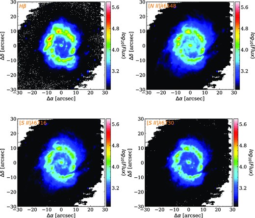
Flux maps of the weaker lines in each emission line group outlined in Table 1. Units are in 10−20 ergs−1 cm−2 spaxel−1 units.
![Corrected flux and LOSVD moments after combining the results from single Gaussian fits with the fits including the secondary component (as explained in Section 2.3). For H α line (left-hand column), and for [N ii]λ6583 line (right-hand column). We display the line flux on a logarithmic scale in units 10−20ergs−1cm−2spaxel−1 (top row), velocity (middle row), and velocity dispersion (bottom row).](https://oup.silverchair-cdn.com/oup/backfile/Content_public/Journal/mnras/524/1/10.1093_mnras_stad1896/2/m_stad1896figa2.jpeg?Expires=1750260140&Signature=k40hwPlTwl4P898VRHRcZGApSJO9KBXNZxsAyaGefc7kgwPtoG~nZMPV-WR9sndwLaIMYHT8u9Du8~zRyP0LlT6xRWUfdHKHUIi6Ugtn2UTBeJg9JB5P1gaFYgYKbhEjxNwxaNzfITOqb4dQ8BI4vtU43J9NgGo8hLH-P~3u2azH4tByQl6QhlZxZtHpniKxmxrLYdR~6lElVEHyF22fi5jF4QgpVNydFfv8ZfHo9tYr5MMhE6n7mXU2fEQu6UXU5H4sEvHcoh7T6tngp4MhKgjSvu~rqF3yVFZ-1bJRcWfQYQgEt-G5e~Z34U-HY~3iFUrR01aaj7hbo05fjt52bg__&Key-Pair-Id=APKAIE5G5CRDK6RD3PGA)
Corrected flux and LOSVD moments after combining the results from single Gaussian fits with the fits including the secondary component (as explained in Section 2.3). For H α line (left-hand column), and for [N ii]λ6583 line (right-hand column). We display the line flux on a logarithmic scale in units 10−20ergs−1cm−2spaxel−1 (top row), velocity (middle row), and velocity dispersion (bottom row).
![Flux and LOSVD moments for fits including higher order moments (h3 and h4). Columns show H α (left-hand column), [N II]λ6583 (middle) and [O III]λ5007 (right-hand column). The units of the flux measurements are 10−20ergs−1cm−2spaxel−1.](https://oup.silverchair-cdn.com/oup/backfile/Content_public/Journal/mnras/524/1/10.1093_mnras_stad1896/2/m_stad1896figa3.jpeg?Expires=1750260140&Signature=uxrHmHxABzVOYQ-JeBt3sOFjL0yRZD6Vw92e5k7~d9CjuicbltwUAJSTizZJtBDDeghKq1jD~dy1sbHA2tSlfbGS6NEGla-581WWN9w9dXOnJRXr2tq97DJRk1-b~lk52R6ISFhw0rLA6UoRalIFgWBleVbqjIlJp71kYhXqzgeXlNGaoqomNIQYLwURzbIrWCsIo45TWBOoNYI436QNL2jioz3l4letq5m7HOkwMX0uoaAH89KNP~NcgniMzZ0EA4HTLfXWAvVqx1XQFxLv0aY11t305hKxuvjnLl-oSnbMWgwEz7gtRdLp1t3kjmfIO7r0V0fIlcbHaOTsTl3Gzw__&Key-Pair-Id=APKAIE5G5CRDK6RD3PGA)
Flux and LOSVD moments for fits including higher order moments (h3 and h4). Columns show H α (left-hand column), [N II]λ6583 (middle) and [O III]λ5007 (right-hand column). The units of the flux measurements are 10−20ergs−1cm−2spaxel−1.
