


ABSTRACT
We describe the first grid-based simulations of the polar alignment of a circumbinary disc. We simulate the evolution of an inclined disc around an eccentric binary using the grid-based code athena++ . The use of a grid-based numerical code allows us to explore lower disc viscosities than have been examined in previous studies. We find that the disc aligns to a polar orientation when the α viscosity is high, while discs with lower viscosity nodally precess with little alignment over 1000 binary orbital periods. The time-scales for polar alignment and disc precession are compared as a function of disc viscosity, and are found to be in agreement with previous studies. At very low disc viscosities (e.g. α = 10−5), anticyclonic vortices are observed along the inner edge of the disc. These vortices can persist for thousands of binary orbits, creating azimuthally localized overdensities and multiple pairs of spiral arms. The vortex is formed at ∼3–4 times the binary semimajor axis, close to the inner edge of the disc, and orbits at roughly the local Keplerian speed. The presence of a vortex in the disc may play an important role in the evolution of circumbinary systems, such as driving episodic accretion and accelerating the formation of polar circumbinary planets.
1 INTRODUCTION
Protoplanetary discs are produced during the star formation process. Stars are frequently formed in pairs or clusters during the collapse of a molecular cloud (Kouwenhoven et al. 2007; Duquennoy & Mayor 2009), and so discs around multiple stars are expected to be common (Monin et al. 2007). Analogous to how circumstellar protoplanetary discs can give rise to planets, the circumstellar and circumbinary discs in a binary star system may act as the birthsites of the satellite(S)- and planetary(P)-type circumbinary planets, respectively (Dvorak 1986). Observations of binary star systems at different evolutionary stages have revealed different types of protoplanetary discs and planetary systems, including circumbinary discs (Simon & Guilloteau 1992; Czekala et al. 2017; Kennedy et al. 2019; Bi et al. 2020; Kraus et al. 2020), individual circumstellar discs (Cruz-Sáenz de Miera et al. 2019; Keppler et al. 2020), and exoplanet systems in both S- and P-type orbits (e.g. Doyle et al. 2011; Martin 2018).
Binary and higher order star systems exhibit rich dynamics that are not seen in single-star systems. The gravitational torque from the inner binary creates a region of dynamical instability, limiting the range of stable orbits for S- and P-type planets (Holman & Wiegert 1999; Quarles et al. 2018; Chen, Lubow & Martin 2020). Companion stars on faraway orbits can perturb the system over long time-scales, causing orbiting particles to undergo von Zeipel–Lidov–Kozai oscillations (von Zeipel 1910; Kozai 1962; Lidov 1962). For simplicity, we restrict most of the discussion in this paper to the binary case.
For circumbinary or P-type orbits around a circular orbit binary, misalignment of the orbit to the binary orbital plane causes the orbit to nodally precess about the binary angular momentum vector. If the inner binary is eccentric, a second stable configuration exists in which the orbiting body precesses about the binary eccentricity vector in a polar orientation (Verrier & Evans 2009; Farago & Laskar 2010; Doolin & Blundell 2011). For circumbinary discs around the eccentric binary, inclination damping due to viscous forces causes the disc to settle at either 0° or 90°, depending on the initial misalignment. This can lead to the creation of polar discs, where the disc is aligned perpendicular to the orbits of the binary stars. The stability of these two orientations has previously been confirmed using analytic theory and smoothed particle hydrodynamics (SPH) numerical simulations (Martin & Lubow 2017, 2018; Lubow & Martin 2018; Zanazzi & Lai 2018; Smallwood et al. 2019).
A handful of such ‘polar discs’ have been observed. The HD 98800 system is a hierarchical double binary system with a circumbinary disc observed around the B binary component (Kennedy et al. 2019). The A and B binary systems orbit each other on a 67 au orbit with moderate eccentricity (e ∼ 0.5), while the disc-hosting BaBb binary components orbit on a 1 au orbit with high eccentricity (e ∼ 0.8; Zúñiga-Fernández et al. 2021). The HD 98800 B disc is truncated on both edges by the inner and outer binary, with the dust disc extending between 2.5 and 4.6 au (Kennedy et al. 2019). More recently, a polar circumbinary disc was observed around V773 Tau B (Kenworthy et al. 2022). Observations of the IRS 43 system (Brinch et al. 2016) have found an edge-on circumbinary disc with the binary star components orbiting outside of the circumbinary disc plane. Both components of the binary are also surrounded by circumstellar discs, each at a different angle to the circumbinary disc, suggesting complex accretion from the circumbinary disc onto the central stars.
To date, all simulations of polar discs have been performed using SPH (e.g. Martin & Lubow 2017; Cuello & Giuppone 2019; Kennedy et al. 2019; Smallwood et al. 2019; Martin et al. 2022). These simulations typically make use of over 106 particles and are able to capture the global dynamical evolution of the disc. However, the range of viscosities that can be included in SPH simulations is limited by the number of particles in a given region. The minimum disc effective viscosity (Shakura & Sunyaev 2009) is roughly α = 0.01 for most simulations (Price et al. 2018). Protoplanetary discs around single stars have been found with viscosities of α ≲ 10−4 (Pinte et al. 2016; Villenave et al. 2022), and so the study of how polar discs behave at lower viscosities is important but has been unexplored.
In this paper, we work to expand on previous results using a grid-based hydrodynamic code to simulate the circumbinary disc. This allows us to extend the results of previous works to lower viscosities than have previously been examined using SPH simulations. This paper is organized as follows. In Section 2, we outline our computational set-up. Our results are presented in Section 3. We discuss the implications to circumbinary disc evolution in Section 4, and conclude in Section 5.
2 METHODS
We simulate a circumbinary disc using the grid-based hydrodynamical code athena++ (Stone et al. 2020), using spherical polar coordinates (r, θ, ϕ) for the simulations. Fig. 1 shows a visualization of our simulation set-up. A disc that begins with an inclination in the range for polar alignment evolution nodally precesses about the binary eccentricity vector. Therefore, we place the binary in the xz-plane of the simulation, so that the binary angular momentum vector |$\boldsymbol{L}_{\rm b}$|points along the positive y-axis and the eccentricity vector |$\boldsymbol{e}_{\rm b}$| points along the positive z-axis. With this placement of the binary, a disc aligning towards a ‘polar’ orientation settles towards the xy-plane of the simulation domain (θ = |$\pi$|/2). This binary orientation keeps the disc from precessing outside of the specified domain during the simulation. This orientation has the additional benefit of orienting the major axes of the binary towards the poles of the spherical polar simulation domain, which prevents strong gravitational interactions from occurring close to the inner radial boundary.
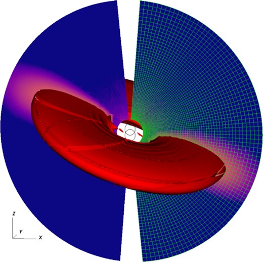
Visualization of the α = 10−2 simulation set-up at t = 1000 binary orbits. The disc starts inclined at t = 0 by rotating the disc along the x-axis, keeping |$\boldsymbol{L}_{\rm disc}$| in the yz-plane, and undergoes nodal precession about the z-axis due to the binary torque. Colours show a slice of density along the xz-plane, with red contour showing a 3D isosurface. The orbits of the binary stars are visible in the centre. The simulation grid is shown at half-resolution on the right half of the simulation domain. Regions close to the binary and the z-axis are not in the computational domain. An animation of the disc evolution is available in the online material associated with this paper and can be downloaded at https://youtu.be/Ny-ggFHALMA.
The binary components are simulated as gravitational bodies, with equal masses m1 = m2 = 0.5, which we place in an eccentric orbit with semimajor axis ab and eccentricity eb. We choose an eccentricity of eb = 0.5. This sets the initial tilt required for disc polar alignment of a low-mass disc to be icrit < i < 180° − icrit, where |$i_{\rm crit}= \arcsin {\sqrt{3/8}} \simeq 38^{\circ }$|, based on the behaviour of test particles (Farago & Laskar 2010). For massive discs, the critical angle changes due to angular momentum exchange between the disc and the binary (Martin & Lubow 2019). Since the binary does not feel the gravitational force from the disc and disc self-gravity is not included from our simulations, the disc can be considered to be in the low-mass regime. We use a second-order leapfrog integrator to solve the equations of motion for the binary. We use the Courant–Friedrichs–Lewy (CFL) fluid time-step of athena++ as the time-step for the integrator.

Schematic of the central binary and circumbinary disc, as well as the angles used to measure the disc orientation. The binary orbits in the xz-plane, with the angular momentum vector |$\boldsymbol{L}_{\rm b}$| pointing along the positive y-axis and the eccentricity vector |$\boldsymbol{e}_{\rm b}$| pointing along the z-axis. The disc is oriented in 3D space by its angular momentum vector |$\boldsymbol{L}_{\rm disc}$|, where it forms an angle i with the binary angular momentum vector |$\boldsymbol{L}_{\rm b}$|. The grey dashed line denotes the disc’s ‘line of nodes’, where the disc crosses the xz-plane at an angle |$\boldsymbol {\Omega }$| with the eccentricity vector |$\boldsymbol{e}_{\rm b}$|.
We initialize the disc at an inclination of i = 120° and ascending node |$\boldsymbol {\Omega }=90^\circ$| with respect to the plane of the binary by converting to tilted disc coordinates (Zhu 2019, equation 44, also see Appendix A). The high initial inclination ensures the disc starts within the librating region that will evolve towards a polar alignment. For test particles around an equal-mass binary, there is no difference between the choice of prograde (60°) versus retrograde (120°) orbits, as the evolution of the test particle only depends on whether the angle between the binary and disc planes is beyond the critical inclination angle icrit. When full three-body systems are considered, angular momentum can be exchanged between the binary system and the circumbinary particle (Farago & Laskar 2010; Martin & Lubow 2019). This creates a difference between the prograde and retrograde cases, and large angular momentum ratios j = Ldisc/Lb can lead to the formation of ‘crescent’ librating orbits (Chen et al. 2019; Abod et al. 2022). Since we do not model the exchange of angular momentum between the disc and the binary, we expect the initially prograde and retrograde cases to be similar.
3 RESULTS
3.1 Polar alignment
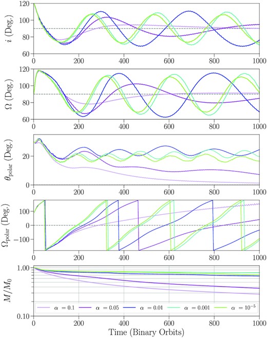
Time evolution of the disc for different values of α, showing large changes in orientation. Top: disc inclination i. Top-middle: longitude of ascending node |$\boldsymbol {\Omega }$|. Middle: angle between the disc and the binary eccentricity vector θpolar. Bottom-middle: longitude of ascending node in the xy-plane |$\boldsymbol {\Omega }_{\rm polar}$|. Bottom: disc mass as a fraction of the initial mass. All angular quantities are measured in reference to the binary orbital plane at a distance of R = 3ab.
Precession of the disc causes |$\boldsymbol {\Omega }_{\rm polar}$| to circulate. As the disc oscillates, inclination damping causes the oscillation amplitude to shrink over time, allowing the disc to settle towards a polar orientation and θpolar to settle towards 0. For fixed disc density and temperature distributions, the time-scale for polar alignment tdamp is inversely proportional to α (King et al. 2013; Lubow & Martin 2018), and so discs with a higher α-viscosity settle towards a polar alignment quicker, performing less oscillations before reaching a polar configuration.
From Fig. 3, the polar alignment time-scale can be estimated to be roughly 300 binary orbits for the α = 0.1 simulation, and roughly 500 binary orbits for the α = 0.05 simulation. This is roughly consistent with the analytical predictions given by equations (29) and (30) of Lubow & Martin (2018), which give tdamp = 220 Tb and 455 Tb, respectively. The difference in density evolution of these two cases likely accounts in part for how tdamp departs from a pure 1/α dependence as α changes. For simulations with viscosities α < 0.05, the oscillation amplitude is not reduced significantly during the course of our simulation time, suggesting that the time-scale for polar alignment is at least on the order of several thousand binary orbits. The polar alignment time-scales for the α = 0.01 simulation are also similar to the SPH simulations with high resolution (106 particles). SPH simulations at lower resolution show a quicker dampening of the tilt oscillations and thus a lower alignment time-scale.
We measure the precession periods in our α = 0.1 and α = 0.01 simulations to be roughly 300–400 binary orbits. The precession period increases over time as the disc material is redistributed outwards. These values are in rough agreement with the SPH simulations of the same Shakura–Sunyaev viscosity1 in Martin & Lubow (2017, 2018, see their equation 2), which measure precession periods of roughly 300 binary orbits for discs that start with a tilt of 80°.
The settling behaviour towards polar alignment is shown clearly in Fig. 4, which plots the trajectory of the disc in the |$i \, \mathrm{\cos \boldsymbol {\Omega }} \!-\! i \, \mathrm{sin\boldsymbol {\Omega }}$| phase space, along with trajectories of test particles in grey. After an initial damping phase, present in all simulations, the disc trajectories spiral inwards towards the point (0.0, 0.5), corresponding to a disc oriented at exactly 90° inclination. High-viscosity discs (α ≳ 0.05) spiral inwards and align towards polar orientation quickly. Discs with lower viscosities (α < 0.05) follow nearly closed oscillating trajectories close to the 70° test particle trajectory, with lower values of α settling towards trajectories slightly closer to a polar orientation. As noted above, the SPH simulations that start at an inclination of 80° with α = 0.01 show a significant decay of tilt over 1000 binary orbital periods.
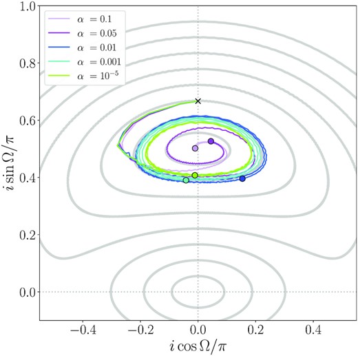
Trajectories of the simulations in |$i\mathrm{\cos \boldsymbol {\Omega }} \!-\! i\mathrm{sin\boldsymbol {\Omega }}$| phase space. Each trajectory starts at the black ‘×’ and spirals inwards counterclockwise towards the point (0.0, 0.5), with the final state of each simulation at 1000 binary orbits marked by the coloured dots. Angular quantities are measured in reference to the binary orbital plane at a distance of R = 3ab, as in Fig. 3. Grey paths show the trajectories of test particle orbits, spaced by 10°. An animation of the test particle precession, as well as the projection onto the phase space, is available with the online version of this paper and can be downloaded at https://youtu.be/ZBkhG6pkOAQ.
Fig. 5 shows the disc surface density profiles at t = 1000 binary orbits. The inner edge of the disc drops off quickly in all simulations at roughly 2a, with higher viscosity discs exhibiting a smaller inner cavity. This behaviour is in agreement with previous numerical simulations (Franchini, Lubow & Martin 2019), as well as analytical predictions (Miranda & Lai 2015; Lubow & Martin 2018), suggesting that discs in a polar orientation should be truncated somewhat closer to the binary than in the coplanar case. The model of Miranda & Lai (2015) suggests that the discs in these simulations should be truncated at the 1:3 commensurability for an outer Lindblad resonance. Streams of gas that flow into the central gap may carry much or all of the gas required for a steady-state accretion disc, as is known in the coplanar case (e.g. Artymowicz & Lubow 1996; Shi et al. 2012; Muñoz & Lai 2016). The profiles generally follow a wider, thinner distribution with increasing α-viscosity. Since the diffusion coefficient ν is proportional to α, the discs with a larger α are able to spread out further due to their shorter viscous time-scale tvisc ∼ R2/ν. As the disc material spreads radially, the change in mass distribution increases the disc’s moment of inertia, increasing the precession time-scale as seen in Fig. 3. Notably, the case of α = 10−5 does not follow this trend, having a slightly wider surface density profile than the α = 10−3 simulation. This may be due to the formation of vortices at low values of α, which generates spiral wakes in the disc. These spirals can increase the outward transport of material and widen the surface density profile. We discuss the details of vortex formation and their impacts on the disc in Section 3.2.
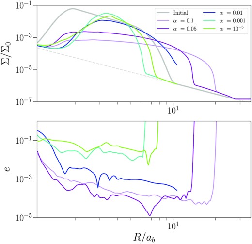
Top: spherically integrated radial surface density profiles at t = 1000 binary orbits, plotted on a logarithmic scale. Bottom: radially averaged disc eccentricity at t = 1000 binary orbits, calculated with equation (16) of Shi et al. (2012).
The bottom panel of Fig. 5 shows the shell-averaged eccentricity of the disc at t = 1000 binary orbits. We calculate the eccentricity of the disc using equation (16) of Shi et al. (2012). The disc eccentricity increases and eventually saturates as time increases, so these values can be taken as a maximum value for each simulation. We find that simulations with α ≳ 0.01 are able to maintain low eccentricities, while discs with lower viscosities are excited to moderate (e ∼ 0.1) eccentricity.
3.2 Vortex formation
A gallery of disc mid-plane density profiles is shown in Fig. 6. Each panel shows a face-on view of the disc at t = 675 binary orbits. Similar to Fig. 5, material in discs with higher viscosity is more spread out with a lower surface density. Some light spiral features are present towards the inner edge of the disc in all simulations, which vary in strength as the disc precesses and changes its orientation relative to the binary, but most of the discs are azimuthally symmetric and largely featureless.
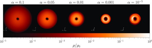
Face-on density profiles of the disc at t = 675 binary orbits.
The notable exception to this behaviour is the nearly inviscid α = 10−5 simulation, which shows a prominent density enhancement along the inner edge of the disc, as well as an associated one-armed spiral. Horseshoe-shaped overdensity features have previously been observed in the Atacama Large Millimeter/submillimeter Array (ALMA) dust-continuum images (Casassus et al. 2013; van der Marel et al. 2013; Casassus 2016), and have been explained by disc material moving on eccentric orbits (Ragusa et al. 2017), or vortices generated by sharp surface density gradients via the Rossby wave instability (RWI, Lovelace et al. 1999; Li et al. 2000). Our simulations are the first instances where vortices have been observed within polar discs. The steep surface density profile along the inner edge of the disc creates a minimum in the local vortensity, an important characteristic in generating RWI vortices (Bae, Hartmann & Zhu 2015). Vortex formation can be suppressed by small amounts of viscosity (α ≲ 10−3; de Val-Borro et al. 2007; Fu et al. 2014; Zhu & Stone 2014; Owen & Kollmeier 2017), so they were not observed in previous SPH simulations of polar discs.
A close-up of the overdensity feature is shown in Fig. 7. We calculate the mid-plane density and vorticity by transforming the disc data as outlined in Appendix A. The left-hand panel shows the disc density, where the overdense region is clearly shown. The right-hand panel shows the local disc vorticity (ω − ω0)/ω0, where ω = −(∇ × vθ) and |$\omega _0 = \frac{1}{2} \Omega _{\rm K}$| is the initial Keplerian vorticity. At the disc mid-plane after the coordinate transformation, the unit vector in θ points downwards, opposite in direction to the unit vector in z, so we add a negative sign to our calculation of vorticity to match the sign convention of vorticity in other coordinate systems, i.e. ω = ∇ × vz. Large areas of anticyclonic motion are coincident with the overdensity region, and confirm that the overdense region is associated with the creation of a vortex. The density cuts across the vortex show that the peak gas density ρmax is enhanced by a factor of ≳8 times the background, which is consistent with previous simulations of RWI vortices (e.g. Lyra et al. 2008; Bae et al. 2015).
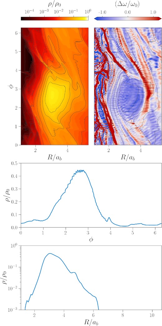
Close-up of the vortex in the α = 10−5 simulation at t = 692 binary orbits. Top-left: gas mid-plane density. The local overdensity and spiral arm pairs are clearly visible. Top-right: local vorticity. Strong anticyclonic regions are indicated in blue. Spiral arms are visible as red diagonal lines in the vicinity of the vortex. In both plots, black curves show contours of density. Middle: azimuthal density across the vortex centre. Bottom: radial density across the vortex centre.
Two spiral arms are visible on the leading side of the overdensity, extending along slanted density contours and trailing inwards towards the star. A similar pair of outward pointing spirals is present along the trailing edge of the vortex, but are less defined, causing the two spirals to partially combine and form a single, wide spiral arm behind the vortex. In the vorticity plot, the spirals are visible in red as diagonal lines of high positive vorticity. Together, these create two distinct pairs of spiral arms originating from the vortex: a ‘central’ pair of spirals, which begin along the centre line of the vortex (roughly 3 ab in the figure) and extend directly away from the vortex, and a ‘tangential’ pair of arms, which are created along the inner and outer radial edges of the vortex and run tangent to the edge of the vortex.
The initial triggering of the RWI and creation of the vortex follows the evolution outlined in Bae et al. (2015). We show panels of the vortex growth and evolution in Fig. 8. The large vortensity minimum at the inner edge of the disc generates several RWI vortices during the linear growth phase of the instability (far left). The number of initial vortices can vary, but our simulations show a consistent m = 2 mode initially present within the first tens of binary orbits. The initial appearance of this mode may be related to the binary components, as previous single-star numerical calculations find the m = 3–5 modes to have the fastest growth rates (Li et al. 2000; Lin 2012). Once the vortices are formed, differences in their orbital speeds will cause them to migrate towards each other and merge (left), eventually forming a single anticyclonic vortex. The merging process is relatively quick, and all vortices are combined into a single vortex within a few hundred orbits of their creation (middle). The remaining vortex persists until the end of the simulation (right). A comparison with the disc density (far right) shows the coincident overdensity and spiral arm features as in Fig. 7.
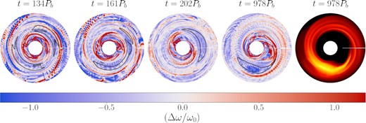
Snapshots of the α = 10−5 simulation, showing the local disc vorticity. In the left-hand four panels, blue regions denote areas of large anticylonic vorticity. The black contours highlight high-density regions (ρ = 0.6ρmax) within the disc mid-plane. Far left: early on, the RWI triggers with an m = 2 mode, creating two vortices on opposite sides of the disc. Left: differences in orbital velocities cause the vortices to move together and merge. Middle: the result is a single vortex that orbits at the inner edge of the disc. Right: the remaining vortex is long-lived, and persists until the end of the simulation. Far right: mid-plane disc density, showing the vortex and the multiple spiral arms. The density scale is shifted compared to Fig. 7 in order to highlight the spiral arms.
The orbital motion of the vortex is shown in Fig. 9. We locate cells of density ρ > 0.5ρmax within the vortex and calculate the average of their locations as the vortex radius and azimuthal position in the local disc coordinates. We also use the radial and azimuthal extent of these cells to calculate the aspect ratio of the vortex χ = rΔϕ/Δr. After the initial vortices merge, the resulting single vortex orbits at roughly three times the binary separation at Keplerian speed. The vortex aspect ratio is somewhat more variable even after the vortices have finished merging, but is generally around a value of χ ∼ 5.
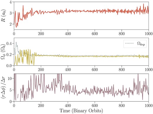
Orbital motion of the vortex in the α = 10−5 simulation. Top: orbital radius of the vortex. Middle: orbital frequency, in units of the binary orbital frequency Ωb. The dotted line shows the Keplerian orbital speed at the vortex’s orbital radius. Bottom: vortex aspect ratio χ = rΔϕ/Δr.
4 DISCUSSION
4.1 The effect of vortices versus lumps in the disc
The overdensity feature observed in the α = 10−5 simulation is noticeably different than similar features created in coplanar circumbinary discs. Several coplanar discs have been found to exhibit horseshoe features, but these features have been explained as a density ‘lump’, created by eccentric gas at the inner edge of the disc interacting with inflow streams created by the action of the binary torque (Shi et al. 2012; Miranda, Muñoz & Lai 2017; Ragusa et al. 2017, 2020). In contrast, the overdensity feature in the polar disc corresponds to the vorticity minimum in the disc, and is closer in nature to vortex-induced clumps caused at the edges of gaps opened by massive planets (de Val-Borro et al. 2007; Zhu et al. 2014; Hammer, Kratter & Lin 2017).
Overdensities in circumbinary discs can drive periodic accretion onto the central binary. Simulations of coplanar circumbinary discs and the binary components by Muñoz & Lai (2016) show the lump at the inner edge causes pulsed accretion at the rate of the lump’s orbital period. When binary eccentricity is included, the accretion flows become pulsed at the rate of the binary orbital period, and can preferentially favour one star for several hundred orbits. In Miranda et al. (2017), mass accretion is found to vary around circular binaries on short time-scales of |$\frac{1}{2} T_{\rm b}$|, as well as on longer time-scales of roughly 5Tb.
Accretion rates in polar discs have been less studied. Smallwood, Lubow & Martin (2022) perform simulations of the HD 98800 system and find that binary accretion rates show no periodicity and are roughly constant in time for a polar disc with α = 0.01. The high viscosity in these simulations means they do not form vortices, even during the passage of the outer AaAb binary.
The vortex in our α = 10−5 simulation exhibits similar variable behaviour on both short and long time-scales. Fig. 10 shows the shell-averaged radial mass flux over roughly 10 binary orbits. Long-term flows are present at distances of 3–4ab, oscillating with a period of roughly 5Tb. This low-frequency mass flux is due to the orbital motion of the vortex around the binary, carrying the overdense region on an eccentric orbit at its local orbital period (Figs 5 and 9). Closer to the binary, at roughly 2ab, short-term outflows are visible with a periodicity of roughly Tb. These outflows are caused by small streams of material pulled from the inner edge of the disc and flung outwards by the binary torque, similar in nature to those seen by Shi et al. (2012). Since our inner binary is eccentric, these streams do not pile-up and form an overdense lump (Miranda et al. 2017). Overall the vortex in our polar circumbinary discs is different from the lump in coplanar circumbinary discs in two ways: (1) the vortex only forms when α is very low, while the lump can form in discs with a much higher α [even in the magnetohydrodynamic (MHD) simulations with α ∼ 0.1; Shi et al. 2012]; (2) the vortex exists in polar circumbinary discs with an eccentric binary, while the lump is only found when the binary is nearly circular (eb ≲ 0.05; Miranda et al. 2017).
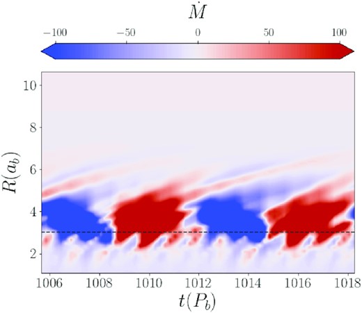
Shell-averaged radial mass flux of the α = 10−5 simulation. The dashed line marks the approximate orbital distance of the vortex. Short-period outflows are visible close to the binary (2ab) as thin red stripes. Long-period variability, associated with the orbital period of the vortex, is visible from 3ab to 4ab as alternating red and blue bands.
The overdensity created by the vortex changes the local pressure gradient on the neighbouring gas, producing regions of super-Keplerian and sub-Keplerian velocity just inside and outside of the vortex orbital radius, respectively (Kuznetsova et al. 2022). These deviations from Keplerian rotation may be observable as a kinematic signature (Boehler et al. 2021), which are inverted but similar in strength to the signatures formed in the gaps of protoplanetary discs thought to be formed by young planets (Teague et al. 2018; Teague, Bae & Bergin 2019; Izquierdo et al. 2022). Future high-resolution studies with ALMA may be able to distinguish vortex creation in polar discs.
Observations of HD 98800 B from Kennedy et al. (2019) show a uniform disc in both gas and dust, with no evidence of large-scale disc asymmetry. The absence of vortex-like features may be a sign that the viscosity in HD 98800 B is high enough to prevent vortices from forming. Another explanation could be that vortices are relatively transient features within the disc. The lifetime of vortices in the disc is on the order of thousands of orbital periods (Zhu & Stone 2014; Hammer et al. 2021). For HD 98800 B, this corresponds to a lifetime of ≲1000 yr for a vortex formed at the inner edge of the disc, which is much shorter than the disc lifetime of ∼10 Myr (Barrado Y Navascués 2006). Therefore, it is possible that any vortices that initially formed in the disc have long since dispersed, unless vortices are continuously generated by the inner binary.
The rightmost panel of Fig. 8 shows the vortex and spiral arms as they appear in the disc. Notably, the appearance of the spiral arms resembles the scattered light images of HD 142527 (Avenhaus et al. 2014, 2017), which is also known to have an overdensity feature (Casassus et al. 2013). Spirals along the inner edge of the disc can be created, without the creation of a vortex, due to the gravitational interaction of the binary with the disc (Price et al. 2018), so it is unclear if vortex-generated spirals are the cause of the spiral arms in HD 142527.
4.2 Prospects for polar circumbinary planets
It is unknown if circumbinary planets are able to form within polar discs. Currently, no planets have been observed in polar orbits around binaries, nor planet candidates in polar-aligned discs. The lack of detections is at least partially due to a strong observational bias; current methods for detecting exoplanets rely on identifying data with multiple, periodic transits, which favour single-star, coplanar systems. Planets on circumbinary orbits exhibit large transit timing variations, on the order of hours or days (Armstrong et al. 2013). Inclined orbits are more likely to produce single or irregular transits due to the orbital precession induced by the binary torque (Martin & Triaud 2014; Chen et al. 2019; Chen, Lubow & Martin 2022), rendering most detection methods used for single planets unusable and requiring the use of special transit folding methods (e.g. Martin & Fabrycky 2021). If circumbinary planets are equally likely to form in polar discs as they are in coplanar discs, they may be as common as planets around single-star systems (Armstrong et al. 2014; Martin & Triaud 2014).
The formation of vortices within low-viscosity discs can have significant effects on planet formation history. An outstanding problem in planet formation involves the formation of large planetary embryos in a disc, as gas drag from the disc can cause growing particles to rapidly spiral inwards onto the star, before they are able to decouple from the gas (Weidenschilling 1977). Anticyclonic vortices in a disc act as grain traps, and can intercept over half of the grains that cross its orbit during their inward radial migration (Fromang & Nelson 2005). Once captured in the vortex, the local vorticity works to focus particles towards the vortex ‘eye’, which can facilitate accelerated growth of planetary material all the way up to Jupiter-mass planets (Klahr & Bodenheimer 2006; Lyra et al. 2008; Zhu et al. 2014; Owen & Kollmeier 2017). In polar discs, vortices may also lead to direct planet formation or seed the disc with a large initial planetesimal population, which can allow further planetary growth and formation terrestrial planets in polar orbits (Childs & Martin 2021, 2022).
Figs 7 and 9 show that the vortex orbits at a few times the binary separation, close to the inner edge of the disc. Indeed, the sharp surface density profile created at the inner cavity wall allows the RWI to produce vortices in the absence of viscosity. This is close to the theoretical stability limit for circumbinary planets (Dvorak 1986). Curiously, many of the circumbinary planets discovered by the Kepler and Transiting Exoplanet Survey Satellite (TESS) orbit just outside the inner stability limit (Martin & Triaud 2014; Welsh et al. 2014). Together, this may suggest a potential in situ formation scenario for close-in circumbinary planets, where the sharp inner cavity of the circumbinary disc generates long-lived vortices that allows for efficient trapping of solid materials. Rapid planet formation at this distance would produce circumbinary planets close to the circumbinary inner stability limit.
5 CONCLUSION
In this paper, we describe the first grid-based simulations on the evolution of polar-aligning circumbinary discs. We find the discs align towards a polar orientation, with time-scales in rough agreement with previous SPH studies and analytic estimates. In nearly inviscid discs, RWI vortices can be generated close to the disc inner edge while polar alignment occurs. These vortices can persist for thousands of binary orbits in a polar disc, and create overdensities within the disc. Two pairs of spiral arms are seen originating from the vortex, along the centre and tangent to the vortex core. The overdensities created by the vortices are fundamentally different from similar features created through eccentricity excitation within the disc. The combination of vortices and spiral arms may create a detectable signature in polar discs, though none have been observed as of yet. The presence of vortices and overdensities in polar circumbinary discs may also aid in the formation of polar circumbinary planets, accelerating planet growth close to the inner stability limit.
SUPPORTING INFORMATION
Please note: Oxford University Press is not responsible for the content or functionality of any supporting materials supplied by the authors. Any queries (other than missing material) should be directed to the corresponding author for the article.
ACKNOWLEDGEMENTS
This paper is based upon work supported in part by UNLV’s Faculty Top Tier Doctoral Graduate Research Assistantship Grant Program (TTDGRA) and the National Aeronautics and Space Administration under grant no. 80NSSC20M0043 issued through the Nevada NASA Space Grant Consortium. ZZ acknowledges support from the National Science Foundation under CAREER grant no. AST-1753168. RGM and SHL acknowledge support from NASA through grants 80NSSC21K0395 and 80NSSC19K0443. Figures in this paper were made with the help of matplotlib (Hunter 2007), NumPy (Harris et al. 2020), and visit (Childs et al. 2012). The animations included in the online version of this paper were made with the help of the NAS Visualization Team.
DATA AVAILABILITY
The data used in this paper are available upon request to the corresponding author.
Footnotes
The equivalent SPH artificial viscosity for these simulations is αSPH = 4 and 0.4, respectively (Lodato & Price 2010).
REFERENCES
APPENDIX A: COORDINATE TRANSFORM OF DISC DATA
Simulations of discs are usually oriented so that their local coordinate axes are aligned with the simulation axes. This alignment simplifies the analysis of important disc parameters such as azimuthal slicing along the mid-plane, or calculation of vorticity along the disc’s vertical axis.
Discs that are inclined, warped, or precess over time are not always aligned with the simulation axes, and so these quantities are harder to acquire without some prior manipulation. We show here our method of manipulating the simulation data of an inclined disc so that it may be analysed in a similar way as a flat, zero-inclination disc. As in the paper, we use spherical polar coordinates for this section, though the basic process can be used for any coordinate system.
Fig. A1 shows an example of the transformation applied to a 2D spherical slice of our simulation data at t = 0. The transformed density and velocity are similar to that of a disc aligned with the coordinate system. Small artefacts are visible in the areas close to the poles of the simulation coordinates due to the lack of initial data in these regions. Small vertical striations can also be seen along the transformed data.
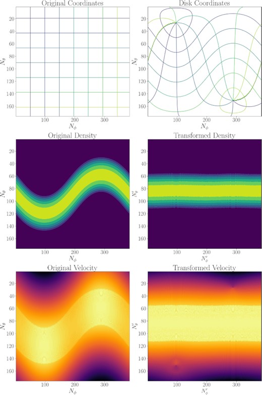
Example of the coordinate transform using a 2D slice of the simulation data at t = 0. Top row: coordinate grid lines for the simulation and disc coordinates. Middle row: disc density in the simulation and disc coordinates. Bottom row: azimuthal velocity vϕ in the simulation and disc coordinates.
For simulations in this paper, we transform the disc data using the total angular momentum vector |$\boldsymbol{L}$| to calculate i and |$\boldsymbol {\Omega }$| using equations (4) and (5). Warped or broken discs can be analysed in a similar fashion by using the local angular momentum vector |$\boldsymbol{L}(R)$| to transform each annulus separately.
