


ABSTRACT
Radiative turbulent mixing layers (TMLs) are ubiquitous in astrophysical environments, for example the circumgalactic medium (CGM), and are triggered by the shear velocity at interfaces between different gas phases. To understand the shear velocity dependence of TMLs, we perform a set of 3D hydrodynamic simulations with an emphasis on the TML properties at high Mach numbers |$\mathcal {M}$|. Since the shear velocity in mixing regions is limited by the local sound speed of mixed gas, high-Mach number TMLs develop into a two-zone structure: a Mach number-independent mixing zone traced by significant cooling and mixing, plus a turbulent zone with large-velocity dispersions which expands with greater |$\mathcal {M}$|. Low-Mach number TMLs do not have distinguishable mixing and turbulent zones. The radiative cooling of TMLs at low and high Mach numbers is predominantly balanced by enthalpy consumption and turbulent dissipation, respectively. Both the TML surface brightness and column densities of intermediate-temperature ions (e.g. O vi) scale as |$\propto \mathcal {M}^{0.5}$| at |$\mathcal {M} \lesssim 1$|, but reach saturation (|$\propto \mathcal {M}^0$|) at |$\mathcal {M} \gtrsim 1$|. Inflow velocities and hot gas entrainment into TMLs are substantially suppressed at high Mach numbers, and strong turbulent dissipation drives the evaporation of cold gas. This is in contrast to low-Mach number TMLs where the inflow velocities and hot gas entrainment are enhanced with greater |$\mathcal {M}$|, and cold gas mass increases due to the condensation of entrained hot gas.
1 INTRODUCTION
Nowadays, the circumgalactic medium (CGM) has become a new frontier in studies of the formation and evolution of galaxies. Many puzzles are still under debate (Tumlinson, Peeples & Werk 2017), among which is the ubiquity of ions peaking at the ‘warm’ temperatures of |$\sim 10^5\, \mathrm{K}$|, such as O vi, detected in quasar absorption sightlines intersecting the CGM (e.g. Tumlinson et al. 2005; Prochaska et al. 2011; Tumlinson et al. 2011; Savage et al. 2014; Lehner, Howk & Wakker 2015; Johnson, Chen & Mulchaey 2015; Keeney et al. 2017; Qu et al. 2020). Such ions are also discovered in high-velocity clouds (HVCs) around the Milky Way Galaxy (e.g. Savage et al. 2014; Tripp 2022). However, the origin and sustainability of these ions are controversial, since gas enriched with O vi at |$\sim 10^5\, \mathrm{K}$| is thermally unstable with a cooling time of |$\sim 10\, \mathrm{Myr}$| much shorter than the dynamic time-scale. One possible origin of O vi is the mixing of cold (|$\sim 10^4\, \mathrm{K}$|) and hot (|$\sim 10^6\, \mathrm{K}$|) phases, given the existence of large amounts of both hot (Li et al. 2008; Fang, Bullock & Boylan-Kolchin 2012; Planck Collaboration et al. 2013; Anderson, Churazov & Bregman 2015) and cold (Stocke et al. 2013; Werk et al. 2014; Prochaska et al. 2017; Cantalupo et al. 2014; Hennawi et al. 2015; Cai et al. 2017) gas in the CGM. The turbulent mixing of two phases, usually accompanied by efficient radiative cooling, could be triggered by the Kelvin–Helmholtz instability occurring at the cold-hot interface with shear flows, which is referred to as so-called radiative turbulent mixing layers (TMLs).
Given both the importance of cooling in TMLs and the ubiquity of supersonic shear flows, it might be intriguing to extend existing studies on radiative TMLs further to supersonic conditions, which motivates this work. We also limit the scope of this work to the weak cooling regime, which is realistic for CGM-like astrophysical environments where the gas pressure and metallicity are relatively low. The outline of this paper is as follows. In Section 2, we describe our numerical methods. We present our results in Section 3, and finally discuss our findings and concludes in Section 4.
2 METHODS
Parameters for the fiducial hydrodynamic simulation. The speed of sound in the hot medium cs = 117.72 km s−1. With δ = 100, the critical Mach number for the KH instability suppression |$\mathcal {M}_\text{crit} = 1.34$|.
| Domain size | Resolution | Metallicity | Number density | Velocity shear | Temperature | Perturbation wavelength |
|---|---|---|---|---|---|---|
| (pc) | (Z⊙) | (cm−3) | (km s−1) | (K) | (pc) | |
| 100 × 300 × 100 | 128 × 384 × 128 | 0.1 | ncold = 10−2 | 100 (|$\mathcal {M} = 0.85$|) | Tcold = 104 | λ = 100 |
| nhot = 10−4 | Thot = 106 |
For the simulations with radiative cooling included, we use a set of cooling functions which assumes collisional and photoionization equilibrium, instead of summing up losses from all the time-dependent ion abundances, since the latter requires excessive memory and computational power. The cooling curves with photoionization are generated by the spectral synthesis code cloudy with background radiation intensity from Madau & Haardt 2005 at the redshift of 0. For more details about the techniques, see Ji et al. (2019, fig. 1).
To study how the Mach number of shear velocity affect the evolution of TMLs, we have run a series of simulations with different initial hot gas velocities, and parameters for which are listed in Table 2. Since the TML thickness can expand significantly with greater Mach numbers, we adopt varying domain heights to ensure the entire TMLs are completely enclosed by the simulation domains. In addition, we carry out adiabatic counterparts for high-Mach number runs to probe the possible impact of cooling on the early growth of turbulence, and a suite of low- and high-resolution simulations for convergence studies, and a few runs with wider simulation boxes to check the effects of box width (x direction), with parameters listed in Table 3. Finally, Table 4 summarizes the notations used in the paper for clarity purposes.
Parameters for simulations with different initial Mach numbers. Other parameters (not listed here) for each run are identical to that for the fiducial case.
| Velocity shear | Mach number | Domain height | Name |
|---|---|---|---|
| (km s−1) | |$\mathcal {M}$| | (pc) | |
| 10 | 0.09 | 300 | M0.09 |
| 20 | 0.17 | 300 | M0.17 |
| 50 | 0.42 | 300 | M0.42 |
| 100 | 0.85 | 300 | FC or M0.85 |
| 200 | 1.70 | 400 | M1.70 |
| 300 | 2.55 | 600 | M2.55 |
| 500 | 4.25 | 800 | M4.25 |
| 800 | 6.80 | 900 | M6.80 |
Parameters for studies of the impact of cooling and resolution. The adiabatic runs are marked with ‘NC’ (no cooling). Other parameters (not listed here) for each run are identical to that for its counterpart in Table 2. We use ΔFC/Δ to represent resolution here (the grid scale of the fiducial run |$\Delta _\text{FC} = 0.78\,$| pc).
| Velocity shear | Feature | Name |
|---|---|---|
| (km s−1) | ||
| 100 | No radiative cooling | M0.85_NC |
| 200 | No radiative cooling | M1.70_NC |
| 300 | No radiative cooling | M2.55_NC |
| 500 | No radiative cooling | M4.25_NC |
| 800 | No radiative cooling | M6.80_NC |
| 100 | Resolution: 0.5 | M0.85_LR |
| 200 | Resolution: 0.5 | M1.70_LR |
| 200 | Resolution: 2.0 | M1.70_HR |
| 300 | Resolution: 0.5 | M2.55_LR |
| 300 | Resolution: 2.0 | M2.55_HR |
| 200 | Box width: 200 pc | M1.70_W2 |
| 200 | Box width: 300 pc | M1.70_W3 |
| 300 | Box width: 300 pc | M2.55_W3 |
Notation system of energy fluxes/rates discussed in this paper.
| Symbol | Description/Definition | Note |
|---|---|---|
| |$\mathcal {L}$| | Radiative cooling rate; |$\mathcal {L}= n^2\Lambda (n,T)$|. | The energy loss rate via radiative cooling (emissivities) |
| |$\mathcal {H}$| | Enthalpy loss rate; |$\mathcal {H}= -\bar{P}\tilde{v}_{i,i}-\left\langle Pv_{i,i}^{\prime } \right\rangle $|. | The rate at which gas enthalpy is being converted to other forms; the angle brackets denote the ensemble averages at the same y coordinate (in our simulations); negative |$\mathcal {H}$| indicates gas expansion, rather than compression. |
| |$\mathcal {D}$| | Turbulent dissipation rate; |$\mathcal {D}\equiv -t_{ij}^\text{R}\tilde{S}_{ij}$|, where |$t_{ij}^\text{R}=-\left\langle \rho v_i^{\prime } v_j^{\prime }\right\rangle $| and |$\tilde{S}_{ij} = \frac{1}{2}\left(\tilde{v}_{i,j} + \tilde{v}_{j,i} - \frac{2}{3}\delta _{ij}\tilde{v}_{k,k} \right)$|. | |$v_i = \tilde{v}_i + v_i^{\prime }$|, |$\left\langle \rho v_i^{\prime }\right\rangle =0$|, where |$\tilde{v}_i$| and |$v_i^{\prime }$| are mean and fluctuating components respectively; |$t_{ij}^\text{R}$| is the Reynolds stress, and |$\tilde{v}_{i,j}$| and |$\tilde{v}_{j,i}$| denote partial derivatives (∂j and ∂i) of |$\tilde{v}_i$| and |$\tilde{v}_j$|, respectively. |
| Q | Surface brightness of radiative mixing layers; |$Q\equiv \int _{y_1}^{y_2} n^2 \Lambda \text{d}y$|. | The cooling region is included in the range from y1 to y2. |
| Fh | Enthalpy flux; Fh ≡ 5/2Pvin. | vin is the inflow velocity of hot gas (with respect to the TML). In our calculation, vin = vy, bot − vy, inter, that is, the inflow velocity is obtained by measuring the gas y-velocity across the bottom boundary of the box vy, bot, relatively to the migrating velocity of the TML interface vy, inter. |
| Fk | Flux of bulk kinetic energy; |$F_\text{k}\equiv \epsilon _\text{k}v_\text{in} = \frac{1}{2}\rho \boldsymbol {v}^2 v_\text{in}$|. | ϵk is kinetic energy density (erg cm−3); specially, the flux into the TML, |$F_\text{k}\sim 5/2Pv_\text{in}\times 1/3\mathcal {M}^2$|. |
| Fh + k | Fh + k ≡ Fh + Fk | When TMLs reach equilibrium, Fh + k ∼ Q (i.e. equation (1)). |
| H | Enthalpy loss rate integrated along y direction; |$H\equiv \int _{y_1}^{y_2}\mathcal {H} \text{d}y$|. | The rate at which enthalpy is consumed through the compression of gas; [y1, y2] accommodates the entire turbulent region, and we choose the bottom and top boundaries as y1 and y2 in our calculation in practice. Note that H ∼ Fh only holds when TMLs reach quasi-equilibrium (equation (9)), while it is not always the case – see Section 3.5 for detailed discussions. |
| D | Turbulent dissipation integrated along y direction; |$D\equiv \int _{y_1}^{y_2}\mathcal {D} \text{d}y$|. | The turbulent region is contained in the range from y1 to y2; D equals to the loss rate of kinetic energy in the whole turbulent region with a unit of erg s−1 cm−2 (can be directly compared with energy fluxes above). Note that since to accurately calculate turbulent dissipation from the definition is tricky, here we instead derive D from the conservation of energy, i.e. to subtract the (kinetic + thermal) energy change due to radiative cooling and inflow/outflow across domain boundaries, from the total energy change integrated over the whole simulation box. |
3 RESULTS
3.1 Short-time evolution: suppression and revival of KH instability
Fig. 1 shows the time evolution of gas density in two representative simulations: the low-Mach number case M0.85 (left) and the high-Mach number case M2.55 (right). For M0.85, it is just the ‘standard’ version of the KH instability with radiative cooling: initial perturbations with long wavelengths grow significantly until secondary instabilities start to appear at |$t\sim 12\, \mathrm{Myr}$|, which results in long-wavelength structure cascading to smaller scales. The TML ultimately saturates with an approximately fixed thickness after |$t\sim 21\, \mathrm{Myr}$|, when the radiative cooling balances the hot-gas entrainment (Ji et al. 2019). However, the high-Mach number case of M2.55 is different in two aspects. First, since there are no unstable modes at |$\mathcal {M}\gt \mathcal {M}_\text{crit}$| (Mandelker et al. 2016), large eddies do not appear at the cold–hot gas interface initially. At |$t\sim 9\,$| Myr, it is from small scales that the TML begins to grow, since the initial long-wavelength perturbations are stabilized by high velocity shears and already damped. Second, in contrast to a fixed thickness in M0.85, the high-Mach number TMLs (M2.55) continues growing in thickness and does not reach a saturation state at least up to |$t \sim 27\, \mathrm{Myr}$|.
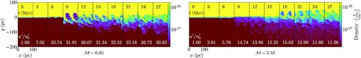
Slice plots of density evolution in M0.85 (left) and M2.55 (right) during the early stage of evolution (|$t\le 27\, \mathrm{Myr}$|), labelled with current evolution time and the turbulent velocity u′ normalized to the magnitude of initial velocity perturbation |$u_0^{\prime }$|. Compared to the low-Mach number case M0.85 where the KH instability is already well-developed at |$t\sim 9\, \mathrm{Myr}$|, the KH instability of long-wavelength perturbations in the high-Mach number case M2.55 is clearly suppressed until |$t\sim 18\, \mathrm{Myr}$| while small-scale turbulence begins to develop earlier.
We investigate the KH instability quantitatively during the initial suppression phase in Fig. 2, where the peak turbulent velocity2 (normalized to the initial velocity perturbation) |$u^{\prime }/u^{\prime }_0$| is plotted as a function of simulation time. Different colours represent runs with different Mach numbers ranging from 0.09 to 6.8, and the solid (dashed) lines are runs with (without) radiative cooling. For low-Mach number cases (|$\mathcal {M}\lt 0.9$|), as expected, the growth rates of turbulence increase with greater Mach number, due to faster growth rate of the KH instability. In contrast, at high Mach numbers, the growth rates become inversely-correlated with Mach numbers, indicating stronger suppression of turbulence at higher Mach numbers when |$\mathcal {M}\gtrsim \mathcal {M}_\mathrm{crit}$|. However, due to the existence of numerical (in our simulations) or physical (in reality) viscosity, the sharp discontinuity in both densities and velocities smooth out, bringing local shears below the critical Mach number, and thus the KH instability revives and triggers turbulence.
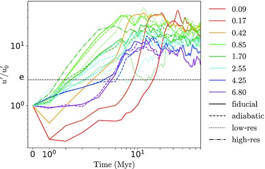
Time evolution of peak turbulent velocity (normalized to the magnitude of initial perturbations) in runs with different Mach numbers ranging from 0.09 to 6.8, represented by different colours. The solid lines refer to runs with radiative cooling included, and the dashed ones are their adiabatic counterparts (i.e. without cooling). The dotted lines are low-resolution runs: M0.85_LR (lime), M1.70_LR (green), and M2.55_LR (aqua), and the two dash-dotted lines are high-resolution runs: M1.70_HR (green) and M2.55_HR (aqua). A factor of e is annotated on the y-axis, indicating the e-folding time of the peak turbulent velocity in each run. As expected, for the three low-Mach number runs, the growth rate increases with raising |$\mathcal {M}$| (shorter te). In contrast, in high-Mach number cases, runs with larger |$\mathcal {M}$| have longer e-folding time, and the effect of radiative cooling on e-folding time is negligible. The e-folding time of turbulence growth is resolution-independent (resolution-dependent) at low (high) Mach numbers.
Besides, since the initial long-wavelength perturbations have already been damped in the high-Mach number case, the KH instability has to grow from smallest scales (where the linear growth rate is maximized) which are determined by the numerical resolution. Therefore, the e-folding time of turbulence growth in high-Mach number cases is unfortunately resolution-dependent: higher-resolution runs where smaller scales are resolved have faster turbulence growth and thus shorter e-folding time compared with their low-resolution counterparts (e.g. see M1.70_LR, M1.70, and M1.70_HR in Fig. 2). However, since the KH instability in low-Mach number cases grows from unsuppressed long-wavelength perturbations, simulations can converge much more easily as long as initial perturbations are well-resolved. Indeed, Fig. 2 shows that the e-folding time in M0.85 and M0.85_LR is comparable, which is expected by the analysis above. We also find that cooling has little influence on the initial stage of turbulence growth, which is consistent with the findings in Ji et al. (2019) that cooling only becomes important in the saturation stage, but not for the ‘kick-off’ of TMLs (which is triggered by the KH instability).
We note that although, as discussed above, the e-folding time of turbulent velocity growth in the high-Mach number case does not converge, TML properties in final saturation stages do converge, which is shown by convergence tests in Section 3.9. For our following discussion, we stick to TML properties in the saturation stage.
3.2 Long-term evolution: morphologies and surface brightness
Fig. 3 shows the time evolution of temperature slices in simulations with Mach numbers ranging from 0.09 up to 6.80. In the run with smallest velocity shear M0.09, the TML barely grows until |$t\gtrsim 140\, \mathrm{Myr}$| with apparently much thinner thickness of |$\sim 20\, \mathrm{pc}$|. With larger velocity shears, the TMLs in M0.42 and M0.85 already develop at |$t\sim 30\, \mathrm{Myr}$| with larger thickness of |$\sim 100\, \mathrm{pc}$|. For supersonic runs of M1.70, M2.55, M4.25, and M6.80, after the initial development of turbulence, we do not find the saturated TML thickness grows significantly with increasing Mach number, for example the run M6.80 has a velocity shear of ∼4 times larger than M1.70, while ultimately only reaches saturated TML thickness of |$\sim 100\, \mathrm{pc}$| which is comparable with M1.70.
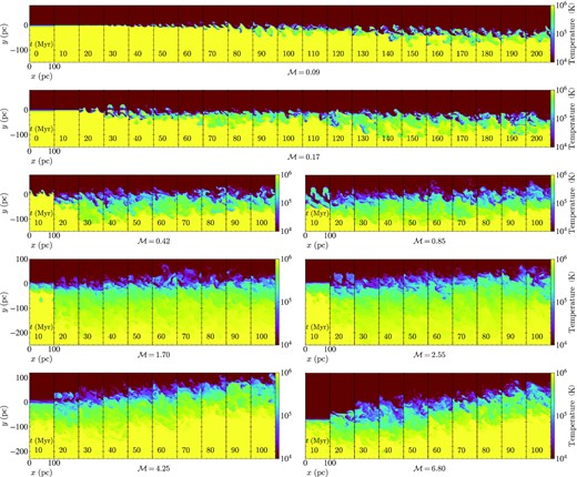
Slice plots of temperature evolution in runs M0.09, M0.17, M0.42, M0.85, M1.70, M2.55, M4.25, and M6.80. For subsonic runs, the saturated mixing layer thickness increases with Mach number, while for supersonic ones, the thickness remains roughly constant. Note: (i) The slices have been cropped accordingly to save space, so the boxes appear shorter than their authentic sizes (regions with little temperature variation are cut off). (ii) Though the intermediate temperature volumes in M1.70 and M2.55 are seemingly more extensive than those in M4.25 and M6.80, their cooling zone widths are actually approximately equal, for the reason that |$T\gtrsim 3\times 10^5\,$| K gas nearly does not cool itself. Meanwhile, the temperature of part of the turbulent zones in M4.25 and M6.80 goes beyond |$10^6\,$| K owing to turbulent dissipation.
Quantitatively, Fig. 4 shows the time evolution of surface brightness Q in simulations with different Mach numbers. In all runs, the saturated surface brightness finally saturates after an initial growth stage ranging from ∼30 to |$100\, \mathrm{Myr}$| (depending on initial Mach numbers), suggesting a steady state is indeed achieved. For subsonic runs M0.09, M0.17, M0.42, and M0.85, the final saturated surface brightness is positively correlated with Mach number, but for supersonic ones, the saturated surface brightness remains at a similar level, regardless of varying Mach numbers ranging from 1.7 up to 6.8. This is consistent with the morphological evolution where the thickness of TMLs ceases increasing with raising Mach number. We will discuss its cause and consequences in the following sections.
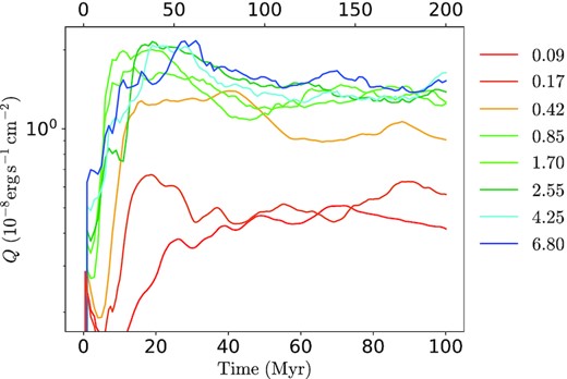
Time evolution of surface brightness from simulations with different Mach numbers (represented by colours). For M0.09 and M0.17, a wider time axis (ranging up to |$200\, \mathrm{Myr}$|) located at the top of the figure is used, since they evolve much slower. All runs reach a steady state with a saturated surface brightness in the final stage. Saturated surface brightness increases with larger Mach numbers at |$\mathcal {M}\lesssim 1$|, while ceases to increase further with Mach numbers at |$\mathcal {M} \gtrsim 1$|.
3.3 Velocity profiles tracing sound speed
According to mixing length theories, turbulent velocities are proportional to local velocity gradients (u′ ∝ ∂vx/∂y), which is demonstrated to be applicable to TMLs by Tan et al. (2021). Therefore, we start with inspecting velocity profiles in Fig. 5, where volume-averaged profiles3 of the bulk velocity vx (solid) and the sound speed cs (dashed) from simulations with different Mach numbers in the saturation stage are plotted. For subsonic runs M0.09, M0.42, and M0.85, the difference between vx and cs narrows with increasing Mach number, while for supersonic runs M1.70, M2.55, M4.25, and M6.80, vx profiles cease to increase with Mach number, after reaching the local sound speed cs in regions with efficient mixing and cooling (which are traced by intermediate sound speed). Apparently, in supersonic cases, profiles of x-velocity are limited and thus shaped by profiles of local sound speed (vx ≲ cs), so the mixing (cooling) regions, as shear layers, have vx, max < cs, h (see vx-cs intersection points in Fig. 5, which roughly indicate positions of boundaries of the cooling region).4
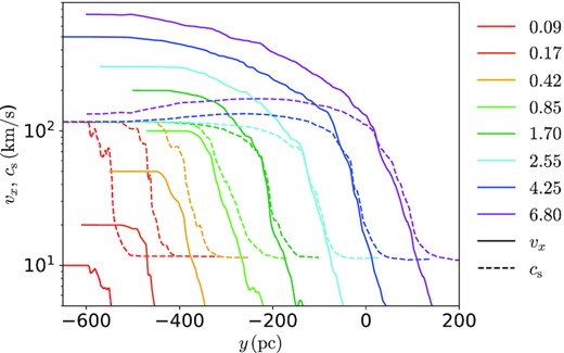
Profiles of x-velocity (solid) and sound speed cs (dashed) in the saturation stage (|$t=80\,$| Myr, except |$t=160\,$| Myr is chosen for the runs M0.09 and M0.17 due to their relatively slow turbulence growth). Apparently in each of these runs, vx does not exceed local sound speed in the mixing region of the TML, which are traced by intermediate sound speed. Particularly, vx curves trace corresponding cs curves in supersonic cases. Note: For clearness, the positions of curve pairs (vx(y) and cs(y)) have been shifted properly along the horizontal axis here, instead of using original coordinates.
Although the problem we study inherently has Galilean invariance which makes velocity gradient rather than the magnitude of velocity matter, we directly plot velocity profiles first, for two reasons: (i) vx, min = 0 in our setup and cs, min is very small (we ultimately compare shapes of profiles that determine gradients, instead of magnitudes, and it makes sense to plot both profiles together if vx and cs have almost the same minimum value), and (ii) it is easier to compare runs with different Mach numbers in this concise plot than a plot of velocity gradients. In case the velocity gradients are of interest, equivalently, we also have them plotted in Fig. 6 (three of the runs), which likewise shows that the gradient of vx (i.e. ∂vx/∂y) is approaching and then tracing ∂cs/∂y with increasing |$\mathcal {M}$| in the mixing (cooling) zone while ∂vx/∂y exceeds (in terms of magnitude) and diverge from ∂cs/∂y outside the cooling zone in high-|$\mathcal {M}$| runs.
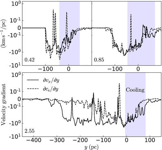
Profiles of the gradients of x-velocity (solid) and sound speed cs (dashed) in the saturation stage (|$t=80\,$| Myr), where regions in which cooling and mixing are significant are shadowed in blue. In the mixing regions, the gradients of vx and cs are almost identical over a factor of 10 in their magnitudes, double-confirming their magnitude profiles closely trace each other in Fig. 5.
3.4 Separation of turbulent and mixing zones
In Fig. 7, we show profiles of velocities (left) and energy rates (right) in simulations M0.42, M0.85, and M2.55. In the left panel are profiles of the bulk velocity vx, turbulent velocity u′ and the local sound speed cs. In all cases, the shear velocity profiles vx do not exceed the local sound speed cs in the cooling region even in the supersonic run M2.55, as already shown in Fig. 5 and double-confirmed here. We also explicitly verified in all cases, that the turbulent velocity profiles are proportional to gradients of vx, which is expected by the mixing length theory mentioned in Section 3.3.5 However, the velocity profiles differ significantly between low and high Mach numbers: in runs M0.42 and M0.85, the highly turbulent regions are roughly co-spatial with the mixing/cooling regions traced by intermediate sound speeds, as expected in traditional ‘turbulent’ ‘mixing’ layers. In contrast, in the high-Mach number run M2.55, the high-turbulent region (shadowed in red) spanning over |$200\, \mathrm{pc}$| develops outside of the mixing region (shadowed in blue), indicating that a TML (the entire turbulent region) at high Mach numbers is characterized by two separated zones, the ‘turbulent zone’ with high-turbulent velocities, and the ‘mixing zone’ with significant mixing and cooling.
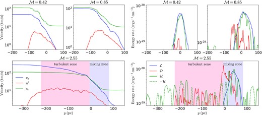
Left panel: profiles (along the y axis) of the shear velocity vx (blue), turbulent velocity u′ (red), and local sound speed cs (green) in the saturation stage (|$t = 80\, \mathrm{Myr}$|) in simulations M0.42 (top-left), M0.85 (top-right), and M2.55 (bottom). Right panel: Profiles of radiative cooling rate |$\mathcal {L}$| (blue), turbulent dissipation rate |$\mathcal {D}$| (red), and the divergence of enthalpy flux (i.e. enthalpy loss rate) |$\mathcal {H}$| (green) with |$\mathcal {H}$| in solid and |$-\mathcal {H}$| in dashed. At low Mach numbers (M0.42 and M0.85), highly-turbulent regions and mixing regions are roughly co-spatial, where the divergence of enthalpy flux compensates radiative cooling in mixing regions. At high Mach numbers (M2.55), the TML is split into two separated zones: the mixing zone (blue shadowed) with strong cooling and predominant turbulent dissipation (the region in which |$\mathcal {L}$| is not below |$\mathcal {L}_\mathrm{max}/10$| in profile is defined as the mixing region here), and the turbulent zone (red shadowed) with large turbulent velocities and weak turbulent dissipation (the boundaries of the turbulent zone here are determined by the ‘hot’ end of the mixing zone and the point at which |$\mathcal {D}$| reaches |$\mathcal {D}_\mathrm{max}/10$| in profile).
The right panel of Fig. 7 shows profiles of the radiative cooling rate |$\mathcal {L}$| (blue), turbulent dissipation rate |$\mathcal {D}$| (red), and enthalpy loss rate |$\mathcal {H}$| (green, refer to Table 4 for detailed definitions of these quantities). The negative values |$-\mathcal {H}$| are also plotted (dashed green), representing enthalpy gain rate due to local gas expansion. In the run M0.42, |$\mathcal {H}$|, and |$\mathcal {L}$| overlap quite well, while |$\mathcal {D}$| is negligible. This indicates the enthalpy flux of hot gas is responsible for balancing radiative cooling in the TML, which is consistent with previous findings (Ji et al. 2019). In M0.85 where the shear flows get close to transonic, |$\mathcal {D}$| becomes significant, that is, turbulent dissipation starts to play a role in energizing the cooling zone. In these two subsonic runs, |$\mathcal {H}$| is still more important than |$\mathcal {D}$| in balancing cooling via radiation. The profiles with significant |$\mathcal {H}$| but negligible |$-\mathcal {H}$| show that the diffuse hot gas tends to be compressed during the process of mixing and radiative cooling, while gas expansion is not considerable.
However, in the supersonic case M2.55 (bottom-right panel of Fig. 7), turbulent dissipation becomes the dominant energy source compensating radiative cooling, while the net contribution from |$\mathcal {H}$| is very tiny (will be clearly shown in Fig. 10). Compared with the mixing zone, turbulent dissipation in the turbulent zone is weaker, although the turbulent velocities in the turbulent zone are higher (as shown in the left panel), which is due to lower densities of hot gas which carry less turbulent energy. The enthalpy loss rate in the TML violently fluctuates between positive and negative values, corresponding to the expansion and compression of gas respectively. The sum of fluctuations in the enthalpy loss rate in the entire turbulent region is much less than turbulent dissipation.
The separation of the turbulent and the mixing zones at high Mach numbers is more than a visual fact; their physical properties are intrinsically different. In the top panel of Fig. 8, we plot the Mach number dependence of turbulent velocities, where the blue and green dots represent the peak turbulent velocities in the entire turbulent region |$u^{\prime }_\mathrm{TML}$|6 and the local turbulent velocities7 in the mixing zone |$u^{\prime }_\mathrm{mix}$|, respectively. At low Mach numbers, both the TML and the mixing zone follow a similar power-law of |$\mathcal {M}^{9/10}$|, that is, their behaviours (dependencies on |$\mathcal {M}$|) are parallel. However, this is not the case for high Mach numbers: the Mach number dependence of |$u^{\prime }_\mathrm{TML}$| follows a power-law of |$\mathcal {M}^{1/3}$| at |$\mathcal {M}\gtrsim 1$|, that is, the increase in shear velocities indeed enhances turbulent motions in the turbulent region. In contrast, |$u^{\prime }_\mathrm{mix}$| becomes independent of |$\mathcal {M}$| at high Mach numbers, indicating that turbulent velocities in the mixing zone cease to increase further with larger initial shear velocities. The bottom panel of Fig. 8 plots the ratio of the turbulent velocity in the mixing zone to that in the entire TML |$u^{\prime }_\mathrm{mix}/u^{\prime }_\mathrm{TML}$|, versus |$\mathcal {M}$| in each simulation. The ratio is independent of |$\mathcal {M}$| at low Mach numbers, while follows |$\mathcal {M}^{1/2}$| at high Mach numbers, further implying that the behaviours of the entire turbulent region and the mixing zone diverge for |$\mathcal {M}\gtrsim 1$|. Consequently, in the supersonic case, the turbulent region grows larger with greater |$u^{\prime }_\text{TML}$| at higher |$\mathcal {M}$|, but the mixing zone does not with an approximately constant |$u^{\prime }_\text{mix}$|, and the mixing zone and turbulent zone become distinguishable.
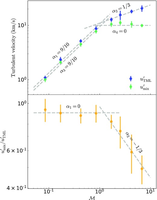
Upper panel: turbulent velocities in the entire TML |$u^{\prime }_\mathrm{TML}$| (blue) and in the mixing zone only |$u^{\prime }_\mathrm{mix}$| (green) plotted against Mach number. Lower panel: the ratio of |$u_\text{mix}^{\prime }$| to |$u_\text{TML}^{\prime }$| plotted against |$\mathcal {M}$|. At |$\mathcal {M}\lesssim 1$|, |$u_\text{mix}^{\prime }/u_\text{TML}^{\prime }$| is independent of |$\mathcal {M}$|, suggesting a mixing zone, if exists, does not distinguish from the whole TML region. However, in cases of |$\mathcal {M}\gtrsim 1$|, |$u_\text{mix}^{\prime }$| and |$u_\text{TML}^{\prime }$| start to follow different power-law relations, indicating that a mixing zone with different properties of turbulence stands out from the TML. Error bars in the figure and hereafter represent one standard deviation of uncertainty around the mean values, which are measured only when the simulations reach the saturation stage.
3.5 Balance of energies
To examine how well the energy balance is maintained, the time evolution of some selected energy fluxes/rates from our simulations are plotted in Fig. 9. Consistent with theoretical predictions above, in subsonic cases (|$\mathcal {M}\lesssim 1$|, top panels of Fig. 9), the sum of enthalpy and bulk kinetic energy flux into the TML Fh + k well balances radiative cooling Q, and the TML reaches quasi-equilibrium described by equations (1) and (8). The contribution from kinetic energy Fk to energizing radiative TMLs is modest compared to enthalpy Fh, that is, the internal energy transported by gas advection and compression is much more significant than turbulent dissipation in balancing radiative cooling.
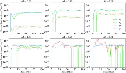
Time evolution of selected mean energy fluxes and rates from simulations with different Mach numbers: the sum of enthalpy flux and bulk kinetic energy flux Fh + k (green-solid), the flux of bulk kinetic energy Fk (green-dashed), the averaged dissipation rate over the whole turbulent region D (red-dotted) and the surface brightness of the TML Q (blue-solid). In subsonic cases, TMLs ultimately reach a quasi-equilibrium state with Fh + k ∼ Q and Fk ∼ D, where turbulent dissipation D is negligible compared to Q. In supersonic cases, however, turbulent dissipation D becomes important and dominant; Fh + k ≲ Q for transonic Mach numbers (M1.70) and Fh + k ≪ Q in highly supersonic runs (M4.25, M6.80), indicating TMLs are not in quasi-equilibrium. Note: the negative fluxes (not shown on logarithmic scales) during the early stage are caused by the initial expansion of the turbulent region (significant turbulent pressure), which is transient and does not imply a steady flux outwards from TMLs.
However, the case is different at high Mach numbers. As shown in the bottom panels of Fig. 9, M1.70 only marginally reaches quasi-equilibrium (Fh + k ≲ Q, Fk ∼ D), whereas M4.25 and M6.80 are far from quasi-equilibrium with Fh + k ≪ Q ∼ D, even when the surface brightness Q is still steady with time. In other words, at high Mach numbers, the mixing zone of the TML is indeed in a steady state characterized by an approximately constant Q, but the relative advection of hot gas to the TML is almost quenched. This non-equilibrium state actually corresponds to the evaporation9 of cold gas, which will be discussed in Section 3.7.
Fig. 10 further shows the surface brightness Q, turbulent dissipation D, and enthalpy loss H taken from simulations with different Mach numbers, plotted against |$\mathcal {M}$| of each simulation. The surface brightness Q scales with |$\mathcal {M}^{1/2}$| for |$\mathcal {M}\lesssim 1$| (consistent with previous findings, e.g. Ji et al. 2019), and saturates for |$\mathcal {M}\gtrsim 1$|. At low Mach numbers, the enthalpy loss H ∼ Q and the turbulent dissipation D is negligible, indicating that low-Mach number TMLs are energized by enthalpy flux. In contrast, at high Mach numbers, turbulent dissipation becomes increasingly dominant with D ∼ Q ≫ H. Although previous studies (Ji et al. 2019) have found turbulent dissipation can become non-negligible with stronger cooling, it is not as predominantly important as the supersonic conditions studied here.
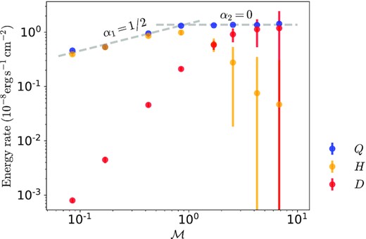
The surface brightness Q (blue), enthalpy consumption H (orange), and turbulent dissipation D (red) plotted against Mach number. At low Mach numbers, TMLs follow |$Q\propto \mathcal {M}^{1/2}$| with the enthalpy as the primary energy source. However, the surface brightness Q becomes independent of |$\mathcal {M}$| at high Mach numbers with increasingly important turbulent dissipation D rather than H that energizes TMLs.
In short, regarding energy balancing, TMLs are distinctively different at low and high Mach numbers. At low Mach numbers, the TML surface brightness scales with |$\mathcal {M}^{1/2}$|. Low-Mach number TMLs are energized by enthalpy flux Fh, and can reach quasi-equilibrium. In contrast, at high Mach numbers, the surface brightness saturates and becomes independent of |$\mathcal {M}$|, and the dominant energy source is turbulent dissipation (sourced from Fk) rather than enthalpy. And a quasi-equilibrium state cannot be reached in high-Mach number TMLs.
3.6 Scaling relations
In this section, we summarize the scaling relations of a few important TML quantities relative to Mach number |$\mathcal {M}$|:
- Turbulent velocity: as already shown in Fig. 8, the turbulent velocity in the entire TML |$u_\text{TML}^{\prime }$| follows the power law (not exact but a fairly good fit):where |$u_\text{TML,1}^{\prime }$| and |$u_\text{TML,2}^{\prime }$| are normalization factors with values of |$u_\text{TML,1}^{\prime }\sim 10.64\, \mathrm{km s^{ -1}}$| and |$u_\text{TML,2}^{\prime }\sim 11.01\, \mathrm{km s^{ -1}}$| measured from our simulations.(10)$$\begin{eqnarray*} u_\text{TML}^{\prime } = \left\lbrace \begin{array}{l l}u_\text{TML,1}^{\prime } \mathcal {M}^{9/10} & \mathcal {M}\lesssim 1 \\ \\ u_\text{TML,2}^{\prime } \mathcal {M}^{1/3} & \mathcal {M}\gtrsim 1 \end{array}, \right. \end{eqnarray*}$$Regarding the turbulent velocity in the mixing zone |$u_\text{mix}^{\prime }$|, where most mixing and cooling occur, Fig. 8 shows:where |$u_\text{mix,1}^{\prime }\sim 9.30\, \mathrm{km s^{ -1}}$| and |$u_\text{mix,2}^{\prime }\sim 10.48\, \mathrm{km s^{ -1}}$|.(11)$$\begin{eqnarray*} u_\text{mix}^{\prime } = \left\lbrace \begin{array}{l l}u_\text{mix,1}^{\prime } \mathcal {M}^{9/10} & \mathcal {M}\lesssim 1 \\ \\ u_\text{mix,2}^{\prime } \mathcal {M}^0 & \mathcal {M}\gtrsim 1 \end{array}, \right. \end{eqnarray*}$$
As already extensively discussed in Section 3.4, both |$u_\text{TML}^{\prime }$| and |$u_\text{mix}^{\prime }$| obey the same power law |$\propto \mathcal {M}^{9/10}$| when |$\mathcal {M}\lesssim 1$|, implying the mixing zone we defined here is indistinguishable from the entire TML region. In the supersonic case (|$\mathcal {M} \gt 1$|); however, unlike |$u_\text{TML}^{\prime }$|, |$u_\text{mix}^{\prime }$| becomes approximately independent of |$\mathcal {M}$|. Again, this suggests that at high Mach numbers, the behaviours of the TML and the mixing zone start to diverge.
- Surface brightness: as a direct indicator of the hot gas entrainment rate, the surface brightness Q is among the key quantities of radiative TMLs. As shown in Fig. 10, the scaling relation for Q is:Combining this relation with equation (10), we have |$Q\propto u_\text{TML}^{\prime 5/9}$| for the subsonic case, which is virtually consistent with the result of Q ∝ u′1/2 obtained in Tan et al. (2021) with weak cooling. But for the supersonic case, Q no longer increase with |$\mathcal {M}$|, though |$u_\text{TML}^{\prime }$| can be enhanced by a larger |$\mathcal {M}$|.(12)$$\begin{eqnarray*} Q \propto \left\lbrace \begin{array}{l l}\mathcal {M}^{1/2} & \mathcal {M}\lesssim 1 \\ \\ \mathcal {M}^{0} & \mathcal {M}\gtrsim 1 \end{array}. \right. \end{eqnarray*}$$
- Inflow velocity: we finally investigate the scaling relation of the inflow velocity vin, which is calculated in a reference frame where the mixing layer is stationary and is shown in Fig. 11 against |$\mathcal {M}$|. The quasi-equilibrium inflow velocity |$v_\text{in}^\text{eq}$| is also plotted which is obtained by combining equation (1) (which assumes a quasi-equilibrium state) and the dependency of Q on |$\mathcal {M}$|, and has the following form:We find that at low Mach numbers, the curve of the quasi-equilibrium inflow velocity |$v_\text{in}^\text{eq}$| well predicts the inflow velocity vin, suggesting that a quasi-equilibrium is reached with |$\mathcal {M}\lesssim 1$|. In particular, at |$\mathcal {M}\ll 1$|, we have |$v_\text{in} \propto \mathcal {M}^{1/2}$|, which has the same Mach number dependence with the surface brightness Q. This further demonstrates that low-Mach number TMLs are primarily energized by the enthalpy of hot gas entrained at an inflow velocity vin. However, at high Mach numbers, the inflow velocity into the TML vin decreases with increasing |$\mathcal {M}$|, indicating hot gas entrainment into the TMLs is significant suppressed under supersonic conditions, even when the TML surface brightness is still comparable with that at transonic Mach numbers (see, e.g. Fig. 10). This is consistent with the energy budget where the enthalpy flux from hot gas entrainment becomes sub-dominant at greater |$\mathcal {M}$| in high-Mach number TMLs (Section 3.5). Moreover, vin falls below |$v_\text{in}^\text{eq}$|, double-confirming that a quasi-equilibrium state cannot be reached for high-Mach number TMLs (as previously discussed in Section 3.5).(13)$$\begin{eqnarray*} v_\text{in}^\text{eq}~\propto \left\lbrace \begin{array}{l l}\displaystyle \frac{\mathcal {M}^{1/2}}{3+\mathcal {M}^2} & \mathcal {M}\lesssim 1\\ \\ \displaystyle \frac{1}{3+\mathcal {M}^2} & \mathcal {M}\gtrsim 1 \end{array}. \right. \end{eqnarray*}$$

Inflow velocity into the TMLs vin (blue dots) plotted against Mach numbers |$\mathcal {M}$|. The dotted purple lines are the equilibrium inflow velocity |$v_\text{in}^\text{eq}$| computed by equation (13), with the assumption of a quasi-equilibrium state described by equation (1), and the dashed-grey lines are the asymptotes of |$v_\text{in}^\text{eq}$| for |$\mathcal {M}\rightarrow 0$| and |$\mathcal {M}\rightarrow \infty$|, respectively. The inflow velocity vin increases with |$\mathcal {M}$| in the subsonic case, but decreases with |$\mathcal {M}$| in the supersonic case. This indicates the entrainment of hot gas relative to the TML is significantly suppressed at high Mach numbers, even when the TML surface brightness still remains constant. The Mach number dependence of vin is well predicted by |$v_\text{in}^\text{eq}$| at low Mach numbers, while falls below |$v_\text{in}^\text{eq}$| at high Mach numbers, suggesting high-Mach number TMLs cannot reach a quasi-equilibrium state.
3.7 Mass evolution of cold gas
As previously discussed, the anticorrelation between vin and |$\mathcal {M}$| at high Mach numbers indicates that the turbulent zone inhibits the hot gas flowing into the TML. Therefore, instead of absorbing the hot gas, in this case, it is the cold gas that is mixed into the TML and evaporates due to strong turbulent dissipation. This is in contrast to the low Mach number case where the hot gas is efficiently entrained and then condenses into the cold gas, and thus the mass of cold phase grows with time. Moreover, at large |$\mathcal {M}$|, since there always exists a net mass influx into TMLs contributed by primarily evaporated cold gas plus (suppressed) entrained hot gas, high-Mach number TMLs cannot reach a quasi-equilibrium state with both the mass and size of TMLs growing with time. But in low-Mach number TMLs, the hot gas entrained into TMLs ultimately condenses into the cold phase through TMLs, and thus TMLs maintain a relatively fixed size and mass, and reach quasi-equilibrium.
Quantitatively, Fig. 12 shows the time evolution of the cold gas column mass density in our simulations, where the colours represent different Mach numbers adopted in each simulation. When calculating the change of the cold gas mass, the increase/decrease caused by the inflowing/outflowing cold gas crossing the top box boundary has been subtracted, so our calculation accurately reflects the cold gas mass evolution caused by TML physics only. The cold gas mass in low-Mach number runs (M0.09, M0.42, and M0.85) appears to grow with time due to the condensation of hot gas into the cool phase. However, at high Mach numbers (M1.70, M2.55, M4.25, and M6.80), the cold gas mass decreases with evaporation rates increasing with greater Mach numbers. The implication for the cloud-crushing problem is that the cloud-wind interfaces can gain mass from hot gas entrainment and condensation, and the cloud tends to survive in a hot wind with lower |$\mathcal {M}$|. But in a higher-Mach number hot wind, when the hot gas entrainment into TMLs is suppressed, the cloud could lose mass from the cloud-wind interfaces due to cold gas evaporation. The tendency of cold gas mass evolution relative to the Mach number is qualitatively consistent with cloud-crushing simulations (e.g. Gronke & Oh 2018).
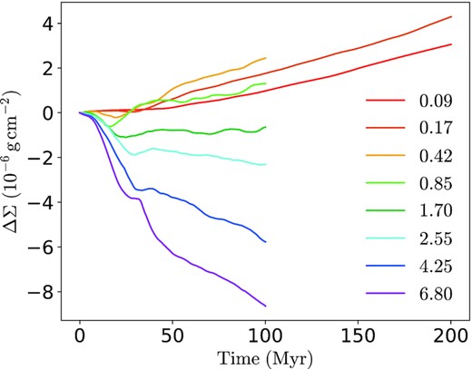
Mass evolution of cold gas in runs with different Mach numbers represented by colours, where ΔΣ is the change in column mass density of the cold gas. The cold gas mass grows with time in low-Mach number runs (|$\mathcal {M}\lesssim 1$|), while decreases with time in high-Mach number runs with evaporation rates increasing with greater |$\mathcal {M}$|.
We finally end this subsection with a closing remark. Our finding that higher Mach numbers lead to faster mass-loss of cold gas in TMLs might sound intuitive and unsurprising. However, this is actually not straightforward on second thought, since based on theories of linear analysis, the KH instability is suppressed under high-|$\mathcal {M}$| conditions, which in principle facilitates the survival and even the growth of cold gas. However, the linear analysis does not deal with the long-term evolution at later times, when the velocity shear in initial conditions smooths out due to finite diffusivity and the evolution with radiative cooling becomes non-linear. Focusing on the long-term evolution, our study presents a physical picture where the cold gas actually suffers from mass-loss via high-Mach number radiative TMLs. In this picture, the inflow velocity and hot gas entrainment into TMLs are indeed suppressed, and this effect actually cuts down further supplement of energy and mass from the hot gas to the TMLs and the cold phase respectively. In the meanwhile, strong turbulent dissipation (the energy is originally from the kinetic energy carried by the hot gas10 entrained into the TML at early times) which powers TMLs evaporates the cold phase. This picture cannot be naively described as larger velocities leading to a stronger KH instability and thus more efficient cold gas mixing in high-Mach number TMLs.
3.8 Ion column densities
We now examine the column densities of typical ions rising from the TMLs in the simulations, where the number density of ions are computed with the assumption of photoionization and collisional ionization equilibrium. Fig. 13 shows the volume-weighted projections the number densities of C iv, S iv, O vi, N v, Si v, and Si vi in M1.70 (|$t = 80\,$| Myr), as well as the corresponding temperature projection. It is shown that these ions closely trace intermediate-temperature gases, which significantly contribute to the mixing layer surface brightness Q. Therefore, it is natural to expect that the saturated ion column densities would follow a power law similar to Q which scales as |$\mathcal {M}^{0.5}$|. Indeed, the steady-state ion column densities do not increase further with Mach number for |$\mathcal {M}\gtrsim 1$|, which is clearly shown in Fig. 14: the ion column densities N follow power laws of |$N\propto \mathcal {M}^{0.5}$| for |$\mathcal {M}\lesssim 1$| and |$N\propto \mathcal {M}^0$| for |$\mathcal {M}\gtrsim 1$|. This is similar to the Mach number dependence of surface brightness Q (Fig. 10) as well.
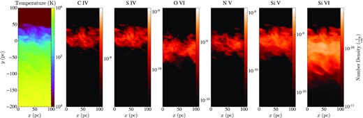
Volume-weighted projections of temperature and number densities of selected typical ions, C iv, S iv, O vi, N v, Si v, and Si vi, in M1.70 at |$t=80\,$| Myr. These ions closely trace the morphology of TMLs with slightly different preferred temperatures and densities.
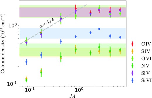
Column densities of C iv, S iv, O vi, N v, Si v, and Si vi plotted against Mach number, with Z = 0.1Z⊙ assumed. The column densities in subsonic runs increase with Mach number for thicker mixing layers, while they appear to be independent of Mach number in the supersonic case with saturated values (shadowed in colours): |$N_\rm{C{\small IV}}\sim 1.77\times 10^{11}\, \rm{cm}^{-2}$|, |$N_\rm{Si{\small V}}\sim 3.56\times 10^{10}\, \rm{cm}^{-2}$|, |$N_\rm{O{\small VI}}\sim 1.68\times 10^{11}\, \rm{cm}^{-2}$|, |$N_\rm{N{\small V}}\sim 3.81\times 10^{10}\, \rm{cm}^{-2}$|, |$N_\rm{Si{\small VI}}\sim 7.32\times 10^{10}\, \rm{cm}^{-2}$|, and|$N_\rm{Si{\small V}}\sim 1.74\times 10^{11}\, \text{cm}^{-2}$|. Note: all ion column densities have been corrected accordingly so that they have identical initial values at different Mach numbers, by cutting off the extra column densities brought by longer boxes (high Mach-number runs), that is, only the effects of radiative TMLs are under study (despite that the contribution from initial conditions are relatively modest).
At low Mach numbers, the magnitudes of ion column densities obtained in our simulations are consistent with previous studies (e.g. Ji et al. 2019). Ji et al. (2019) explored a range of cooling strengths, gas pressures, and metallicities, as well as time-dependent cooling and non-equilibrium ionization, and concluded that under plausible CGM conditions, sightlines penetrating hundreds or thousands of TMLs are required to explain the observed high-column densities (e.g. O vi). Our findings further indicate that due to the saturation at high Mach numbers, the maximum ion column densities from one single TML are still far less than the observed values, and the scenario of hundreds or thousands of TMLs per sightline might be still needed even when these TMLs are highly supersonic.
3.9 Convergence
Previous studies (Ji et al. 2019; Fielding et al. 2020; Tan et al. 2021) using a similar numerical setup have demonstrated that low-Mach number TML are generally well-converged, and here we perform convergence tests under supersonic initial conditions, by comparing both low- and high-resolution runs for two Mach numbers |$\mathcal {M}=1.70,2.55$| against fiducial-resolution ones. Fig. 15 shows the time evolution of the surface brightness of each run. For runs with the same Mach number but different resolutions, although the e-folding time in the growth stage does not converge, the saturated values of surface brightness are similar, indicating the ultimate steady state does not strongly depend on resolution at high Mach numbers. The resolution dependence is quantitatively shown in Fig. 16, where the e-folding time of initial growth of the TML clearly varies with the resolutions (top panel); however, the surface brightness and (column) dissipation rate do converge (middle and bottom panels). We have also verified the convergence of turbulent velocities measured from our simulations.
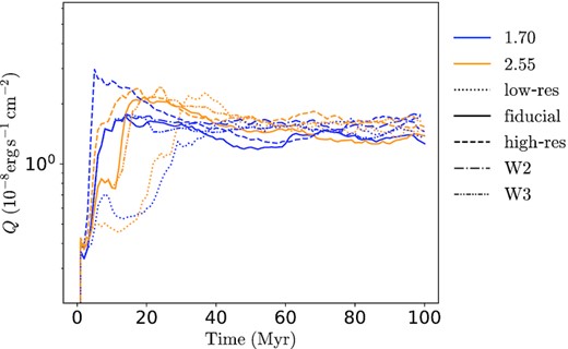
The time evolution of TML surface brightness Q in runs with low (dotted), fiducial (solid), and high (dashed) resolutions, with box widths of 100 pc (solid), 200 pc (dash-dotted), and 300 pc (dash-dot-dotted), and with different Mach numbers of 1.70 (blue) and 2.55 (orange). The steady-state magnitudes of Q in simulations with different resolutions are numerically converged, even though the initial growth rates are not with larger rates under higher resolutions. And Q exhibits negligible dependence on the width of the simulation box.
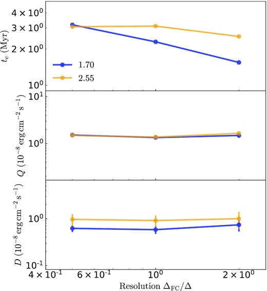
The e-folding time of initial turbulent velocity growth te (top panel), steady-state surface brightness Q (middle panel) and (column) dissipation rate D (bottom panel) in runs with different Mach numbers of 1.70 (blue) and 2.55 (orange), plotted against resolutions used in each simulation. It is clearly shown that te is resolution-dependent while Q and D are well converged.
The non-convergence in the e-folding time is expected based on previous discussion in Section 3.1: since the KH instability of initial large-wavelength perturbations is suppressed at high Mach numbers, the later-developed KH instability has to grow from the smallest wavelengths which are resolved by the finest grid size, so the e-folding time is resolution-dependent. Fortunately, since the steady state is determined by energy advection and balance (Section 3.5) rather than the KH instability, the TML properties after the initial growth stage do converge, and our main findings focusing on steady-state TMLs are thus robust.
In addition, in order to examine the possible effect of finite domain widths which limit the maximum allowed sizes of TML structures, we carry out three simulations with larger domain sizes along the directions with periodic boundary conditions (see Table 3 for parameters), which are denoted by the dash-dotted and dash-dot-dotted lines in Fig. 15. The results demonstrate that varying domain widths do not lead to qualitative change in the saturated surface brightness with variations within a factor of |$\sim 10{{\ \rm per\ cent}}$|, and simulations with fiducial domain widths are numerically robust. The ‘finite domain width effect’ is negligible due to the nature of turbulence cascades from large to small scales: the largest eddies comparable to the domain width at t = 0 do not reform after turbulence is fully developed, and the finite domain widths thus become irrelevant for the TML properties. In fact, we suspect the ‘finite domain width effect’ is even less significant at high Mach numbers, since the KH instability of large, domain-size wavelengths are always stabilized under supersonic conditions as previously discussed.
4 DISCUSSION
4.1 Caveats
In this study, we perform 3D hydrodynamic simulations to investigate properties of the radiative TMLs under the compressive limit. Certain caveats apply to our study:
The strong cooling regime:
This work primarily focuses on the weak cooling regime when the cooling time is longer than the eddy turnover time of the turbulence (τturb/tcool < 1).11 In this regime, the gas at intermediate temperatures produced by TMLs tends to be single-phase, and 1D averaging of fluid properties (temperatures, velocities, energetics, etc.) is representative in our analysis. However, this might not hold in the strong cooling regime, when TMLs become highly multiphase on small scales and form fractal structures (Fielding et al. 2020; Tan et al. 2021); Tan et al. (2021) already demonstrated that TMLs follow different scaling relations in weak and strong cooling regimes. Nevertheless, the weak cooling regime studied in this work is typical for most galactic environments, such as the circumgalactic and intergalactic medium where cooling is inefficient due to low gas pressure and metallicity.
Magnetic fields, cosmic rays, and thermal conduction:
Ji et al. (2019) showed the mixing of phases can be significantly inhibited by magnetic tension, therefore turbulence and column densities of typical ions are correspondingly suppressed. It is plausible that magnetic fields are amplified by small-scale dynamo and suppress TMLs at high Mach numbers as well, while further work is required to address the impact of magnetic fields in the compressive limit. We also did not include cosmic rays, which might pressurize the gas at intermediate temperatures on both small (Wiener, Oh & Zweibel 2017) and large scales (Salem, Bryan & Corlies 2016; Farber et al. 2018; Butsky & Quinn 2018; Ji et al. 2020, 2021; Buck et al. 2020). In addition, thermal conduction (Borkowski, Balbus & Fristrom 1990; Gnat, Sternberg & McKee 2010), especially anisotropic thermal conduction could change the structure of mixing layer as well. Since the magnitudes of thermal conduction in galactic environments is less constrained, here we assume a negligible level of thermal conduction and rely on numerical phase mixing on grid scales. Tan et al. (2021) found the Field length is not necessary to be resolved for convergence, so thermal conduction may not be important for this particular problem, either physically or numerically.
Non-equilibrium ionization and time-dependent cooling curves:
We adopted the assumption of equilibrium ionization and time-independent cooling curves in the simulations for physical simplicity and computational affordability. Though non-equilibrium ionization and time-dependent cooling curves might alter the properties of TMLs, their effects do not make order-of-magnitude differences (Kwak & Shelton 2010; Ji et al. 2019). However, admittedly, these effects might be more important at high Mach numbers, since the dynamical time of TMLs could be even shorter than the ion recombination time. We leave this straightforward improvement for future work.
Survival of cold clouds:
Our conclusion on cold gas mass evolution can be directly applied to shear motions with large coherent length scales, such as jets and cold streams. Although this result is qualitatively consistent with some cloud-crushing simulations, this consistency needs to be viewed with caution, especially in the case of clouds moving supersonically, where a bow shock is produced and the post-shock gas returns subsonic, so supersonic TMLs becomes inapplicable here. In addition, since our simulations do not implement a realistic cold cloud, shock compression and thermalization of the cloud are not captured in the simulations. Therefore, we ask readers to bear this difference in mind when interpreting our results of cold gas survival.
4.2 Conclusions
The key features of low- and high-Mach number TMLs are respectively illustrated by Fig. 17, with detailed conclusions summarized as follows:
Early-stage and long-term evolutions: from the suppression of the KH instability to a steady state:
In the case of |$\mathcal {M}\gt \mathcal {M}_\mathrm{crit}$|, the KH instability of long-wavelength perturbations is initially suppressed, and TMLs can not develop until the jump in shear velocity profile becomes smoothed out and small-scale subsonic turbulence starts to emerge. The growth rate of turbulence in TMLs decreases with increasing |$\mathcal {M}$| for |$\mathcal {M}\gt \mathcal {M}_\mathrm{crit}$|, while increases with greater |$\mathcal {M}$| in the low Mach number case. When TMLs are fully developed, both low- and high-Mach number TMLs ultimately reach a steady state with key quantities (surface brightness, etc.) remaining approximately constant with time. At high Mach numbers, although the initial growth rate of turbulence is not numerically converged (since large-wavelength perturbations are stable to KH instability and turbulence has to grow from ‘hard-to-resolve’ small scales), TML properties in the steady state do converge numerically.
Saturated surface brightness and ion column densities in high-Mach number TMLs:
When TMLs reach a steady state, the surface brightness Q and ion column densities N (|$N_O\, \small{\rm VI}$|, etc.) in each simulation are measured, and our findings are as follows. At |$\mathcal {M}\lesssim 1$|, both Q and N scale with Mach number with a power law of |$\mathcal {M}^{0.5}$|, while at |$\mathcal {M}\gtrsim 1$|, neither Q nor N increases further with greater |$\mathcal {M}$|, indicating a saturated level of surface brightness and ion column densities in high-Mach number TMLs, for example |$N_O\, \small{\rm VI}$| saturates at |$\sim 10^{11}\, \mathrm{cm^{-2}}$| (0.1Z⊙ assumed). Therefore, the scenario proposed in Ji et al. (2019), that each sightline penetrating hundreds or thousands TMLs is required to explain the high O vi column densities in the CGM possibly holds at even much higher shear velocities as well.
A high-Mach number TML consisting of a turbulent zone and a mixing zone:
We find that the shear velocity profiles of TMLs are shaped and constrained by local sound speeds in the zone with prominent mixing. Under supersonic conditions, this constraint from local sound speeds prevents both the turbulent velocity and size of the mixing zone from growing further with larger Mach numbers, while outside of the mixing zone, turbulence in the hot gas continues to accumulate with increasing Mach number. As a consequence, a high-Mach number TML develops into a turbulent zone with large turbulent velocities which expands with greater |$\mathcal {M}$|, plus a mixing zone with significant gas cooling and phase mixing. Unlike the turbulent zone, quantities associated with the mixing zone (e.g. surface brightness Q, ion column densities N) are independent of |$\mathcal {M}$|. The mixing zone has intrinsically different gas dynamics from the entire high-Mach number TML: turbulent velocities in the entire TML |$u^{\prime }_\mathrm{TML}$| and the mixing zone |$u^{\prime }_\mathrm{mix}$| follow different power-law relations: |$u^{\prime }_\mathrm{TML}\propto \mathcal {M}^{1/3}$| and |$u^{\prime }_\mathrm{mix} \propto \mathcal {M}^0$|, respectively. In contrast, at low Mach numbers, the mixing zone is indistinguishable from the entire TML region, with both |$u^{\prime }_\mathrm{TML}$| and |$u^{\prime }_\mathrm{mix}$| follow the same power law of |$\mathcal {M}^{9/10}$|.
Energy supplement: enthalpy consumption versus turbulent dissipation:
At low Mach numbers, TMLs are primarily powered by local enthalpy consumption against radiative cooling, and turbulent dissipation is negligible. However, approaching to higher Mach numbers, turbulent dissipation becomes increasingly dominant in energizing TMLs, while the net contribution from enthalpy consumption becomes less important. It is also worth mentioning that although the turbulent zone is featured by large velocity dispersions, in terms of energies, it contains relatively weaker turbulent dissipation due to much lower densities of the hot gas; the turbulent dissipation actually peaks at the connecting region between the turbulent and mixing zones.
Suppression of both inflow velocity and hot gas entrainment at high Mach numbers:
Under the assumption of a quasi-equilibrium state where the influx of enthalpy and kinetic energy balances radiative cooling, the inflow velocities of hot gas has asymptotes of |$v_\text{in}^\text{eq}~\propto \mathcal {M}^{1/2}$| for |$\mathcal {M}\rightarrow 0$| and |$v_\text{in}^\text{eq}~\propto \mathcal {M}^{-2}$| for |$\mathcal {M}\rightarrow \infty$|. This implies the inflow velocity as well as hot gas entrainment is enhanced by larger shear velocity at |$\mathcal {M}\lesssim 1$|, but is substantially suppressed at |$\mathcal {M}\gtrsim 1$|. Moreover, the measured inflow velocity vin is well-predicted by |$v_\text{in}^\text{eq}$| for |$\mathcal {M}\lesssim 1$|, but falls below |$v_\text{in}^\text{eq}$| for |$\mathcal {M}\gtrsim 1$|, indicating high-Mach number TMLs do not reach a quasi-equilibrium state.
Hot gas condensation and cold gas evaporation in low- and high-Mach number TMLs, respectively:
Low-Mach number TMLs are accompanied by efficient hot gas entrainment. The hot gas condenses into cold phase via mixing, powering TMLs against radiative cooling and leading to the increase of cold gas mass. In contrast, the inflow velocity and hot gas entrainment are suppressed at high Mach numbers. Driven by strong turbulent dissipation in TMLs, cold gas evaporates and is ‘digested’ by TMLs, with a mass-loss rate increasing with higher |$\mathcal {M}$|.
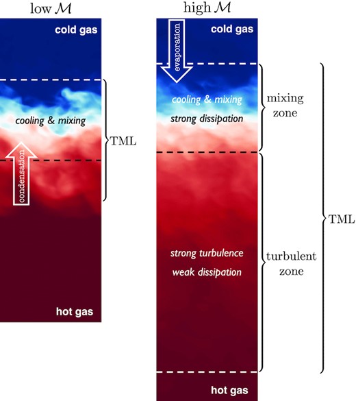
Schematic diagram illustrating the key features of low- and high-Mach number TMLs – see the texts for details.
ACKNOWLEDGEMENTS
YY is grateful to his girlfriend Yuening Zhao for all her love and encouragement. The authors thank the anonymous referee and the editor for the constructive comments and suggestions which significantly improve this work. The authors also thank Chad Bustard, Max Gronke, Philip Hopkins, Linhao Ma, Peng Oh, Brent Tan, Zhiyuan Yao, and Feng Yuan for helpful discussions. The authors are supported by the Natural Science Foundation of China (grants 12133008, 12192220, and 12192223), the science research grants from the China Manned Space Project (No. CMS-CSST-2021-B02) and a Sherman Fairchild Fellowship from Caltech. The simulations were performed on the High Performance Computing Resource in the Core Facility for Advanced Research Computing at Shanghai Astronomical Observatory, the Wheeler cluster at Caltech and allocations FTA-Hopkins/AST20016 supported by the NSF and TACC. We have made use of NASA’s Astrophysics Data System. Data analysis and visualization are made with python 3, and its packages including numpy (Van Der Walt, Colbert & Varoquaux 2011), scipy (Oliphant 2007), matplotlib (Hunter 2007), the yt astrophysics analysis software suite (Turk et al. 2010), the absorption spectra tool Trident (Hummels, Smith & Silvia 2017), and the spectral simulation code cloudy (Ferland et al. 2017).
DATA AVAILABILITY
The data supporting the plots within this article are available on reasonable request to the corresponding author.
Footnotes
By following the choice of Tmix (thus tcool, mix) in Tan et al. (2021), we can calculate the Damköhler numbers in our simulations (see Section 4.1). Though tcool, mix defined here is relatively large, the evolution times we use (|$\ge 100\,$| Myr) have turned out to be sufficient for a saturated state of the mixing layer to arise. In case the cooling time for the geometric mean of hot and cold temperatures is of interest, |$t_\text{cool} = 10\,$| Myr for |$T=10^5\,$| K.
In practice, following Ji et al. (2019), we use the vy velocity dispersion |$\delta v_y \equiv \sqrt{\langle v_y^2 \rangle - \langle v_y \rangle ^2}$| to measure the turbulent velocity, in order to exclude the contribution of the bulk shear velocity predominantly along the x-direction.
Since τturb < tcool, the TML with slow cooling (‘well-stirred reactor’) appears to be single-phase (Fig. 3, see also fig. 7 of Tan et al. 2021), that is, the temperature distribution of a certain slice (fixed y) of gas is relatively uniform; therefore, volume-averaged profiles are able to track local fluid properties fairly accurately. In contrast, fast cooling produces multiphase mixing layers (Tan et al. 2021), where averaged values might not be representative.
More precisely, as the hot boundary of the cooling zone has |$T\sim 3\times 10^5\,$| K, the shear velocity of the well-developed cooling zone |$v_{x,\text{max}}\sim c_\text{s}(3\times 10^5\, \text{K})\sim 0.55c_\text{s,h}$|.
Though it is not so clear in the figure with logarithmic scales (Fig. 7), the proportionality u′ ∝ ∂vx/∂y is obvious in linear scales.
Since the turbulent zone does not remarkably distinguish from the mixing layer within the entire turbulent region in the subsonic case, we compute the turbulent velocity in the entire turbulent region rather than that ‘turbulent zone’ we define. As in Tan et al. (2021), the peak turbulent velocity is measured to characterize the TML.
We define the local (peak) turbulent velocity of the gas in the mixing zone as the turbulent velocity of the gas enriched with O vi at |$\sim 3\times 10^5\,$| K (in practice, we pick up gas at 2-|$4\times 10^5\,$| K).
D + H = Q is literally the integral form of the energy equation from the time-independent hydrodynamic equations, assuming the sum of gas internal energy in the turbulent region does not change, |$-t_{ij}^\text{R}\tilde{S}_{ij}-\bar{P}\tilde{v}_{i,i}-\left\langle Pv_{i,i}^{\prime } \right\rangle = n^2 \Lambda$| (in the frame where the cold-hot interface is static – see Table 4 for detailed notations).
The non-equilibrium state is intuitively expected in the case of evaporation, since a flow of ‘hot gas condensing into cold gas’ in equilibrium cannot form when the cold phase is being continuously absorbed and evaporated by the TML which causes a continuous growth of the TML.
An equivalent statement given Galilean invariance could be: the energy is originally from the bulk motion of the hot phase relative to the cold phase.
The runs with weakest turbulence (M0.09 and M0.17) have Damix ∼ 1, while the others with higher |$\mathcal {M}$| have Damix < 1 or even ≪1, which means most of our simulations are in the weak cooling regime.
