


ABSTRACT
Previous studies have shown that the normalization and scatter of the galaxy ‘main sequence’ (MS), the relation between star formation rate (SFR) and stellar mass (M*), evolves over cosmic time. However, such studies often rely on photometric redshifts and/or only rest-frame UV to near-IR data, which may underestimate the SFR and M* uncertainties. We use MAGPHYS + photo-z to fit the UV to radio spectral energy distributions of 12 380 galaxies in the COSMOS field at 0.5 < z < 3.0, and self-consistently include photometric redshift uncertainties on the derived SFR and M*. We quantify the effect on the observed MS scatter from (1) photometric redshift uncertainties (which are minor) and (2) fitting only rest-frame ultraviolet to near-infrared observations (which are severe). At fixed redshift and M*, we find that the intrinsic MS scatter for our sample of galaxies is 1.4 to 2.6 times larger than the measurement uncertainty. The average intrinsic MS scatter has decreased by 0.1 dex from z = 0.5 to ∼2.0. At low z, the trend between the intrinsic MS scatter and M* follows a functional form similar to an inverse stellar mass-halo mass relation (SMHM; M*/Mhalo versus M*), with a minimum in intrinsic MS scatter at log (M*/M⊙) ∼ 10.25 and larger scatter at both lower and higher M*, while this distribution becomes flatter for high z. The SMHM is thought to be a consequence of feedback effects and this similarity may suggest a link between galaxy feedback and the intrinsic MS scatter. These results favour a slight evolution in the intrinsic MS scatter with both redshift and mass.
1 INTRODUCTION
The galaxy main sequence (MS) describes the empirical relation between the star formation rate (SFR) of galaxies and their stellar masses (e.g. Daddi et al. 2007; Noeske et al. 2007; Speagle et al. 2014; Whitaker et al. 2014; Renzini & Peng 2015; Barro et al. 2017; Leslie et al. 2020; Thorne et al. 2021). These studies find that galaxies have higher SFR with increasing redshifts at a fixed stellar mass (M*) in the earlier universe, and more massive galaxies have higher SFRs at a fixed redshift. Some of these studies show a flattening or turnover in the relationship at high masses (log (M*/M⊙) > 10.5) (e.g. Whitaker et al. 2014; Leslie et al. 2020; Thorne et al. 2021), and suggest that this turnover is driven by the quenching of star formation due to feedback processes.
The galaxy MS is a powerful tool for understanding and constraining the distribution and evolution of galaxies (Katsianis et al. 2020; Curtis-Lake et al. 2021; Daddi et al. 2022; Popesso et al. 2023). According to theories of galaxy feedback, the existence of a relatively tight MS is thought to be mainly driven by the dynamical balance between inflows and outflows caused by self-regulated star-formation and/or active galactic nuclei (AGN; Somerville & Davé 2015). Characterizing this evolution is difficult because observations only provide a single snapshot in time for each observed galaxy. However, the evolution in the scatter, slope, and normalization in the MS of large statistical samples of star-forming (SF) galaxies with cosmic time provides an indirect way to study galaxy evolution. The width (or scatter) of the MS at a single redshift is thought to reflect the burstiness of the average star formation history (e.g. Guo et al. 2013; Schreiber et al. 2015; Santini et al. 2017; Caplar & Tacchella 2019; Donnari et al. 2019; Katsianis et al. 2019; Matthee & Schaye 2019). Theories suggest that a small MS width (small scatter, e.g. ∼0.1 dex) is indicative of gradual, continuous star formation histories (SFHs). In contrast, large MS widths (large scatter, e.g. ∼0.4 dex) are indicative of more bursty, stochastic SFHs (e.g. Tacchella et al. 2016; Sparre et al. 2017).
The question around whether the intrinsic MS scatter is constant or evolving is actively debated. Previous studies have found a time-independent MS scatter (e.g. Daddi et al. 2007; Noeske et al. 2007; Whitaker et al. 2012; Ciesla et al. 2014; Speagle et al. 2014; Pessa et al. 2021), while others suggest it evolves with redshift (e.g. Kurczynski et al. 2016; Santini et al. 2017; Katsianis et al. 2019; Davies et al. 2022; Shin et al. 2022). As the width of MS is related to the SFH, the MS scatter can provide useful constraints on the evolution of SF galaxies. For example, a larger burstiness or stochasticity in the SFH can lead to an increase in MS scatter, and this may change over cosmic time (Matthee & Schaye 2019).
Improving our understanding of the galaxy MS and its scatter requires using large samples of galaxies with accurate redshifts. However, it is observationally expensive to get spectroscopic redshifts for every galaxy. A common solution is to instead use photometrically derived redshifts (zphot). Most previous studies of the galaxy MS have relied on determining stellar masses and SFRs based on SED-fitting at fixed photometric redshift zphot and ignore the uncertainty of the zphot (e.g. Speagle et al. 2014; Leslie et al. 2020; Thorne et al. 2021). Studies that do not account for zphot uncertainty will systematically underestimate the uncertainties in all distance-dependent parameters (e.g. M* & SFR).
In this study, we use MAGPHYS + photo-z (Battisti et al. 2019) to study the intrinsic scatter of the MS. The improvement in using MAGPHYS + photo-z is that it sets zphot as an unknown quantity and finds its probability distribution (Battisti et al. 2019). Hence, the uncertainty in the zphot is incorporated into the overall uncertainty in the derived physical properties of the galaxy. This allows us to examine how much of the scatter in the MS is driven by measurement uncertainty as opposed to true intrinsic MS scatter or other measurement uncertainties. Simultaneously, MAGPHYS + photo-z also includes IR information to resolve the effect of dust attenuation at UV-near-IR wavelengths on the SED based on dust emission from mid-IR-radio, which dramatically improves the accuracy of the derived properties, particularly for SFRs (Battisti et al. 2019). Therefore, the unique aspect of MAGPHYS + photo-z is that it uses broad-band photometry to predict the best-fitting properties in a self-consistent manner, which helps to mitigate potential biases on the derived values.
This paper is organized as follows: Section 2 introduces the data and methods used in this study, Section 3 summarizes our results, and Section 4 compares our results with some previous observational studies and simulations, and Section 5 outlines our conclusions. Throughout this paper, the flat Lambda cold dark matter (ΛCDM) model is adopted by assuming the Hubble constant is H0 = 70 km s−1 Mpc−1, and the mass density of the Universe is Ωm, 0 = 0.3.
2 DATA AND METHODS
2.1 COSMOS sample
The multiwavelength observations of galaxies used in this study come from two catalogues: the COSMOS2020 catalogue (Weaver et al. 2022) and the COSMOS Super-deblended catalogue (Jin et al. 2018). The COSMOS2020 catalogue contains photometric data for ∼1 million sources in 13 filters from UV to near-IR (Weaver et al. 2022), and the COSMOS Super-deblended catalogue presents photometric data for ∼200 000 galaxies in 11 filters in the mid-IR, far-IR, and radio (Jin et al. 2018). We cross-match the galaxies’ ID and select a subsample of galaxies with SEDs that are sampled well enough to constrain their stellar mass and (dust-corrected) SFRs robustly. To achieve this, we use two criteria: (1) signal-to-noise ratio (S/N) of S/N > 3 in three or more UV–near-IR bands and (2) S/N > 3 in two or more IR–radio bands. By virtue of criterion (2), all of the sources in our sample have a match in the Super-deblended catalogue.
It is important to note that criterion (2) roughly translates into a cut in SFR such that only galaxies above a certain SFR will be included. This SFR threshold increases as a function of increasing redshift (see Section 2.2.4). Additionally, AGNs are excluded based on X-ray detections and IR & radio colour cuts (Seymour et al. 2008; Donley et al. 2012; Kirkpatrick et al. 2013). This is done because MAGPHYS + photo-z does not include AGN models, so the derived properties are not accurate for these sources. Due to the limited availability of data required for these AGN diagnostics, some AGNs may not be identified and removed. Further details and references on these cuts are in section 3.3 of the Battisti et al. (2019). These selection criteria leave us with a photometric sample of 14 607 galaxies. For later comparison (Section 3.1.1), only 3873 of the whole 14 607 galaxies have spectroscopic redshifts (zspec).
2.2 Methods
2.2.1 MAGPHYS + photo-z
MAGPHYS fits the full SEDs of galaxies with known redshifts from the ultraviolet to the radio (da Cunha, Charlot & Elbaz 2008; da Cunha et al. 2015) by combining the emission from stellar populations with the attenuation and re-emission of starlight by interstellar dust. The recent MAGPHYS + photo-z extension, described in Battisti et al. (2019) extends the code to fit the SEDs of galaxies with unknown redshifts, and constrain the photometric redshift simultaneously with other galaxy physical properties. In practice, the code builds libraries of model UV-to-radio SEDs at different redshifts and compares them with the observed SEDs of galaxies, using a Bayesian method to obtain the likelihood distributions of physical parameters such as redshifts, stellar masses, and SFRs. There are two sets of libraries used in MAGPHYS + photo-z: (1) an optical library that describes emissions from stars, and (2) an infrared library that describes the emission from dust. The optical library uses the spectral population synthesis models of (e.g. Bruzual & Charlot 2003) and initial mass function from (e.g. Chabrier 2003); while the infrared library consists of models for PAHs and hot dust emitting in the mid-IR, and warm and cold dust components in thermal equilibrium that emit in the far-IR to submillimeter (da Cunha et al. 2008). These two sets of model libraries maintain the balance of the energy absorbed by dust (via attenuation in UV to near-IR) and the energy re-emitted by dust (via thermal emission in mid-IR to sub-mm). Due to insufficient models at z < 0.4 to compare to based on the redshift prior that is adopted in the MAGPHYS + photo-z, galaxies with zphot < 0.4 are not constrained well. Therefore, we exclude galaxies with zphot < 0.4 after running the code (Battisti et al. 2019). An example MAGPHYS + photo-z fit is shown in Fig. 1. We compare the distributions of photometric redshifts of our sample with those of the full COSMOS2020 sample in Fig. 2.
![Output of MAGPHYS + photo-z for one of the galaxies of our sample, COSMOS2020 ID 1587. The upper panel shows the best-fit SED (black curve), the observed data (red square) and the predicted unattenuated SED (blue curve). The black open circle on the SED fitting curve is the corresponding model photometry. The goodness of fit is presented by χ2 in the upper right corner. The lower panel shows the likelihood distribution of 10 basic physical parameters: zphot, stellar mass (log [M*/M⊙]), log [SFR/(M⊙ yr−1)], specific-SFR (log [sSFR/yr]), dust luminosity (log [Ldust/L⊙]), dust mass (log [Mdust/M⊙]), mass-weighted stellar age (log [Agem/yr]), V-band dust attenuation (AV/mag), 2175$\mathring{\rm A}$ bump strength ($E_{\rm b}^{\prime }$), and the effective dust temperature (Tdust/K) (Battisti et al. 2019).](https://oup.silverchair-cdn.com/oup/backfile/Content_public/Journal/mnras/520/1/10.1093_mnras_stad108/3/m_stad108fig1.jpeg?Expires=1750207675&Signature=vpkUeavWS5HIGTDa0tJa7P0YEwuZ~-qv7MnfdS3XpSexWrW8wL~4W2EGHDRNH9NVlhWKJ2Lh~rMxMB5wN5JzrPc4RK7PxK-JPc0MIPzfxHf-bOsq9xhI70B6ZVkLoi7di136oMQNEkFWXWU3OKo1GOEbPlS0Pavb54SZ4wuJXVYpDgonM9FRMUv4-94L~OOiG3YmA6BhwNqvwf1r-A2n-mzbpAs9zQNy9S6-Byj9clKKOBKyZq1qjzKwvcPffJEO0XWDT~oSfnxrIA~bKChWC3rlPTCT0xk-pHGh21nvIVxXVNXMcqHMLKaDjVGT8fSEJ7Ttf8B3R0PpLmEK08YgHg__&Key-Pair-Id=APKAIE5G5CRDK6RD3PGA)
Output of MAGPHYS + photo-z for one of the galaxies of our sample, COSMOS2020 ID 1587. The upper panel shows the best-fit SED (black curve), the observed data (red square) and the predicted unattenuated SED (blue curve). The black open circle on the SED fitting curve is the corresponding model photometry. The goodness of fit is presented by χ2 in the upper right corner. The lower panel shows the likelihood distribution of 10 basic physical parameters: zphot, stellar mass (log [M*/M⊙]), log [SFR/(M⊙ yr−1)], specific-SFR (log [sSFR/yr]), dust luminosity (log [Ldust/L⊙]), dust mass (log [Mdust/M⊙]), mass-weighted stellar age (log [Agem/yr]), V-band dust attenuation (AV/mag), 2175|$\mathring{\rm A}$| bump strength (|$E_{\rm b}^{\prime }$|), and the effective dust temperature (Tdust/K) (Battisti et al. 2019).
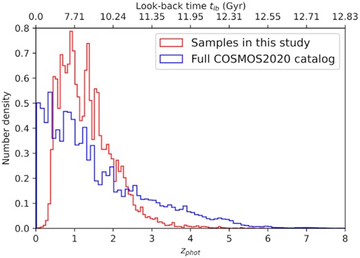
Normalized zphot histogram for the galaxies. The red histogram indicates the distribution of photo-z’s from MAGPHYS + photo-z for the 14 607 galaxies in our sample, while the blue histogram represents the parent distribution of the whole 964 506 galaxies from COSMOS2020 catalogue (Weaver et al. 2022), where the zphot are derived using LePhare (Arnouts et al. 2002; Ilbert et al. 2006). We show the corresponding look-back time tlb on the top axis.
We fit the SEDs of 14 607 galaxies with MAGPHYS + photo-z to determine the M*, SFR, zphot and respective errors. We use the χ2 value of the best-fitting model from MAGPHYS + photo-z as an indicator of the goodness of fit. We fit the χ2 distribution with a lognormal function (see Fig. 3) and convert the lognormal parameters μ and σ to the geometric parameters μgeo and σgeo. Finally, we perform a 2σ confidence cut (i.e. χ2 < μgeo + 2σgeo) to the histogram and remove the high-χ2 cases. The remaining galaxies are reduced to 13 639, and their χ2 ≤ 4.76.
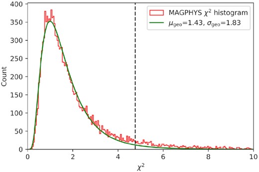
Distribution of MAGPHYS + photo-z fit χ2 of our 14 607 galaxies. The black curve represents the normalized lognormal distribution function fitting to the χ2 histogram, while the vertical black dashed line indicates the normal 2σ confidence cut within χ2 ≤ 4.76.
2.2.2 Reference MS relation
Although the goal of this study is not to investigate the relation between SFR and M*, we note that the exact functional form of the MS is still under debate (e.g. Katsianis, Yang & Zheng 2021; Leja et al. 2022). Different methods of estimating SFRs are thought to be the primary reason for differences between studies (Katsianis et al. 2020). Hence, despite using similar catalogues from the COSMOS field as Leslie et al. (2020) that use radio continuum for robust SFRs (dust-insensitive), there are some other systematic problems that can arise, such as priors, metallicities, time-scales, stellar masses, ages, etc. We stress that the reference MS we show is intended only to guide the eye, and we do not use it for any selection cuts (i.e. to define ‘on’ versus ‘off’ the MS), which instead are based on sSFR (see Section 2.2.3). Therefore, the choice of the reference MS has no impact on the results of this study.
2.2.3 sSFR selection
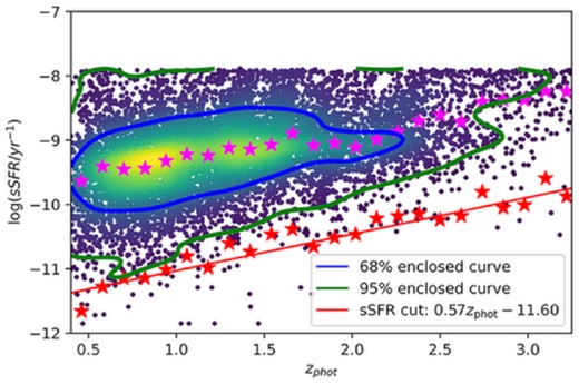
log (sSFR) versus zenclosed contour plot for the 13 071 selection galaxies within 2σ − χ2 from redshifts 0.4 to 3.25. The colours ranging from blue to yellow indicate the increasing number density. The number of galaxies inside the enclosed blue and green curve is 68 (1σ) and 95 per cent (2σ) of the total population, respectively. The magenta points indicate the median value of log (sSFR/yr−1), while the red points are the median-3σ values for 24 sSFR bins. The red line is the sSFR cut adopted in this study, and there are 64 galaxies identified as quenched galaxies. Due to the minimum time-scale of star formation in MAGPHYS + photo-z, there is a maximum value of log (sSFR/yr−1) ∼ −8, corresponding to the adopted SFR time-scale (100 Myr), showing as a horizontal boundary in the diagram.
2.2.4 Influence of IR-selection on SFR- and mass-completeness
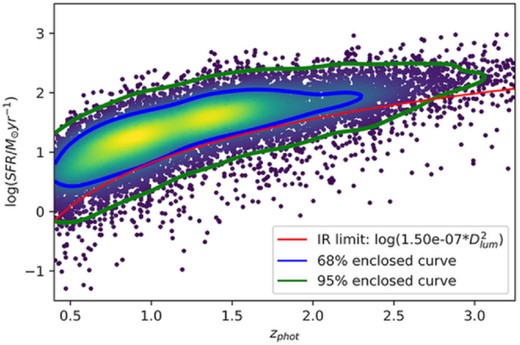
log (SFR) versus z enclosed contour plot for the 13 071 selection galaxies within χ2 selection from redshifts 0.4 to 3.25. The equation (4) is plotted as the red curve in this diagram.
Due to the detection limits, we cannot trust our ability to detect galaxies that are below equation (4) in Fig. 5. This SFR incompleteness translates to an incompleteness on stellar mass (via galaxy MS relation). We infer the corresponding mass-completeness threshold at each redshift using the Leslie et al. (2020) MS relation. For subsequent analysis, we will refer to samples above and below this threshold as our mass-complete and mass-incomplete samples, respectively.
3 RESULTS AND ANALYSIS
3.1 The role of redshift uncertainty and IR data on the measured scatter of the MS
In this study, we use MAGPHYS + photo-z to constrain the stellar masses and SFRs of our galaxies because it uses the full wavelength range from UV to radio, and it constrains the photometric redshifts jointly with the other physical parameters. Using the full SED provides the tightest possible constraints on M* and SFR, thus minimizing the MS scatter that is due to errors on these parameters. Obtaining the photometric redshift at the same time allows us to fold in the redshift error into the errors on M* and SFR. This improves our ability to quantify the ‘observational’ scatter on the MS and, in turn, characterize its intrinsic MS scatter. In this section, we test the accuracy of MAGPHYS + photo-z and quantify the influence that the redshift precision and inclusion of IR data have on derived physical properties (for the COSMOS filter set).
3.1.1 Accuracy of zphot relative to zspec
To examine the zphot accuracy of MAGPHYS + photo-z, we use the latest COSMOS master spectroscopic catalogue (curated by M. Salvato for internal use within the COSMOS collaboration), which is the same data set used to originally test the code (Battisti et al. 2019). There are spectroscopic redshifts, zspec, for 3873 out of the 14 607 galaxies in our sample. After applying the χ2 cut, we obtain 3724 galaxies. Here we adopt some metrics defined in section 4.1.1 of Battisti et al. (2019) to estimate the accuracy of zphot. We find σNMAD = 0.086, |$\eta = 4.2{{\ \rm per\ cent}}$|, and zbias = −0.002, where σNMAD (normalized median absolute deviation) is known as the precision or scatter of the data, η characterizes the fraction of catastrophic failures, and zbias represents the accuracy of the redshift (i.e. systematic deviation or bias). The value of zbias is much smaller than σNMAD, and hence we constrain the redshifts very well with the multiple UV to radio bands. Since we use a similar data base as the one used in Battisti et al. (2019), the results of σNMAD, η, and zbias should be similar. As a comparison, these values calculated in Battisti et al. (2019) are σNMAD = 0.032, η = 0.037, zbias = −0.004 for the COSMOS2015 samples, respectively.
The upper panels of Fig. 6 is a demonstration of zphot accuracy of MAGPHYS + photo-z, which also shows a comparison between the M* and SFR derived from zphot and zspec. The median values of differences for M* and SFR are 0.00 and 0.05 dex, respectively, reflecting that MAGPHYS + photo-z does not affect the overall measurement of M* and SFR. Therefore, we do not expect that relying on zphot will introduce significant bias or dominate the uncertainty of the other derived properties.
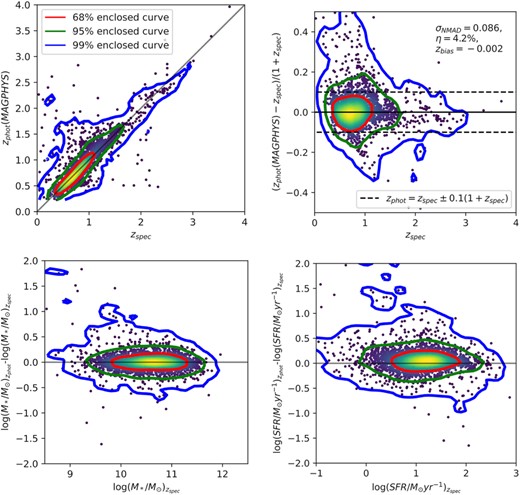
Upper left-hand panel: Comparison of measurement uncertainties between default MAGPHYS high-z (i.e, fixed to zspec) and MAGPHYS + photo-z runs for the subsample of 3724 χ2-selection galaxies with spectroscopic redshifts. Upper right-hand panel: redshift accuracy ((zphot − zspec)/(1 + zspec)) as a function of zspec. The redshift scatter (σNMAD), catastrophic failure rate (η), and redshift bias (median((zphot − zspec)/(1 + zspec))) values are shown at the upper right corner. Lower panels: Difference in M* and SFR derived by zphot and zspec as a function of the zspec-derived values. The 2D histogram/scatterplot colours range from blue to yellow with increasing number density. The black line in each subdiagram is the one-to-one relation as reference; red, green, and blue curves enclose 68, 95, and 99 per cent populations of sample galaxies within 2σ-χ2 cut.
3.1.2 Uncertainties of zphot, M*, and SFR
We characterize the measurement uncertainties of zphot, M*, and SFR for our sample of 13 418 galaxies in Fig. 7. In our analysis, the data are separated into five bins of M* with a width of ≥0.5 dex at a specific redshift epoch. The uncertainty in M* in each bin is ∼0.06 dex, while the zphot uncertainty is ∼0.05. Both uncertainties are ∼10 times smaller than the bin size in this study (≥0.5 dex for log (M*) bin and ∼0.5 for redshift epoch) therefore we do not anticipate that these uncertainties will have a substantial impact on the derived intrinsic scatter on the MS. The median value of SFR’s uncertainty is 0.08 dex, which is comparable to the scatter of galaxies on the MS (e.g. ∼0.2 dex; Speagle et al. 2014). Thus, when measuring the intrinsic scatter of MS, we need to consider SFR’s uncertainty as the component of the scatter in MS and remove it properly to obtain the intrinsic MS scatter. Our method for removing this component is described in Section 3.2.

Distribution of the values and uncertainties for the key parameters of our study for the 13 418 galaxies in our sample. Red, green, and blue curves enclose 68, 95, and 99 per cent populations of sample galaxies within 2σ-χ2 cut. The median values of zphot, log (M*/M⊙) and log (SFR/M⊙ yr−1) are 1.20, 10.64, and 1.42, while the median values of uncertainties are 0.05, 0.06, and 0.08 dex, respectively.
3.1.3 Contribution of including IR data to the uncertainties of M* and SFR
IR wavelengths probe dust emission and provide information regarding the amount of dust-obscured star formation. By excluding IR observations from the SED fits, we can determine the impact of these bands on the uncertainties of M* and SFR. We rerun the MAGPHYS + photo-z without fitting the observational data for filters at wavelengths longer than IRAC2 (4.5 |$\mu$|m) for the same 14 607 galaxies. After rejecting the cases with bad fits (χ2 > 2σ), we compare the uncertainties of zphot, M*, and SFR derived from UV to near-IR photo-z fitting to those results from fitting the full available SED in the top panels of Fig. 8. As expected (Battisti et al. 2022), the non-IR fits tend to come with larger measurement uncertainties because fewer observations are available to constrain the models. For zphot and M*, including the IR bands only leads to a relatively small improvement (i.e. decrease) in the uncertainty. In contrast, for SFR, the median uncertainty when IR bands are not included is nearly 2.5 times larger than that with the IR bands. This is because the IR bands are important to distinguish the amount of dust-obscured star formation. It is harder to accurately measure the intrinsic scatter of the MS with the larger measurement error in SFR. Therefore, by restricting the sample to sources where SED fitting can be performed that include IR filters, we significantly reduce the amount of scatter of the MS arising from measurement uncertainty to accurately constrain the intrinsic MS scatter. The lower panels of Fig. 8 show the difference in the values of zphot, M*, and SFR with and without the IR bands included. It can be seen that the median of the difference remains close to zero as a function of each property suggesting that there is minimal bias occurring as a result of the MAGPHYS + photo-z priors.
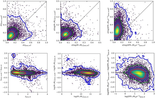
Upper panels: Comparison between the uncertainties on zphot, M*, and SFR for MAGPHYS + photo-z runs including IR bands (labelled ‘phot, IR’) and without IR or radio bands (‘phot, non-IR’). Differing from the cases for zphot and M*, the SFR’s uncertainty increases dramatically for SED fits without the IR data. The median uncertainty values derived from MAGPHYS + photo-z including the IR bands (distributed along x-axis) are 0.05, 0.06, and 0.08 dex for zphot, M*, and SFR, while the median uncertainty values derived from non-IR runs (distributed along y-axis) are 0.08, 0.08, and 0.25 dex, respectively. The black line in each subdiagram is the one-to-one relation as reference; red, green, and blue curves enclose 68, 95, and 99 per cent populations of sample galaxies within 2σ-χ2 cut. Lower panels: Difference in measurements between the SED fits with and without IR bands included as a function of the measurements derived from fitting including IR bands. For the COSMOS2020 data, we find that the dominant factor in accurately constraining the scatter in the MS is whether the IR bands are included to constrain the dust-obscured SFR.
3.2 Measuring the intrinsic MS scatter
We divide our sample into six redshift bins: |$z_{{\rm phot}} = 0.5,\ 1.0,\ 1.5,\ 2.0,\ 2.5\ \&\ 3.0$|, with widths of Δz = 0.5 except for the lowest bin, which spans 0.4–0.75 due to the limitation on the redshift prior for MAGPHYS + photo-z (Section 2.2.1). At each redshift, we further divide the sample into five stellar mass bins. We determine the log (SFR) dispersion (standard deviation) of the galaxies within each bin relative to the median log (SFR) measurement uncertainties. We set the following five bins for all selected galaxies according to their mass: log (M*) < 9.5 log (M⊙), 9.5–10.0 log (M⊙), 10.0–10.5 log (M⊙), 10.5–11.0 log (M⊙), and >11.0 log (M⊙). The values adopted for each bin is the median log (SFR) and M* of each group. We characterize the intrinsic MS scatter in the range of 0.4 < zphot < 3.25 (see Fig. 2). The upper boundary (zphot = 3.25) corresponds to where our sample size dramatically decreases such that we do not have enough sources to properly characterize the MS scatter. Then we take the further selections of 2σ-χ2 and sSFR cut (see Sections 2.2.1 and 2.2.3) to reduce the effects of quiescent galaxies on the intrinsic MS scatter.
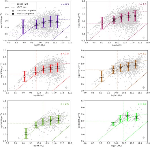
M*–SFR relation of our galaxies in six redshift bins. All bins are shown through 13 071 selection galaxies with colours from purple to red to green coding the range of zphot at 0.5, 1.0, 1.5, 2.0, 2.5, and 3.0. The horizontal dot–dashed line indicates the IR-selection completeness cut in SFR, and the vertical dashed line indicates the corresponding IR-selection completeness cut in M*. The open symbols indicate the mass-incomplete data. We drop the data points where the numbers of galaxies within a bin are less than 50. The longer error bars indicate the standard deviation of the SFR distribution in each stellar mass bin, while the shorter black ones represent the median MAGPHYS measurement uncertainties. The grey error bar in the bottom right of each panel denotes the median uncertainties on M* (along the x-axis) and SFR (along the y-axis) from MAGPHYS + photo-z for the entire redshift bin. The curves are the MS relations at each redshift epoch from Leslie et al. (2020). The maximum value of log (sSFR/yr−1) ∼ −8 due to the adopted SFR time-scale shows as an upper boundary of the slope in each SFR–M* panel, while the bottom right slope represents the sSFR cut at each redshift.
‘N’ is the number of galaxies, ‘σtot’ is the galaxy SFR dispersion (standard deviation), ‘σmeas’ is the MAGPHYS uncertainty in SFR, and ‘σint’ is the intrinsic MS scatter in each M* bin. The mass-incomplete data are marked as ‘–’, but the number of galaxies in the binning interval are still shown. Since all the M* < 9.5 log (M⊙) galaxies lie in the mass-incomplete regime, they are not included in the table.
| M* | |$9.5\!-\!10.0\log({\rm M}_{\odot })$| | |$10.0\!-\!10.5 \log({\rm M}_{\odot }$|) | |$10.5\!-\!11.0 \log({\rm M}_{\odot })$| | |$\gt 11.0\log({\rm M}_{\odot }$|) | ||||||||||||
|---|---|---|---|---|---|---|---|---|---|---|---|---|---|---|---|---|
| zphot | N | σtot | σmeas | σint | N | σtot | σmeas | σint | N | σtot | σmeas | σint | N | σtot | σmeas | σint |
| 0.5 | 428 | 0.36 | 0.09 | 0.34 | 897 | 0.35 | 0.08 | 0.34 | 922 | 0.40 | 0.07 | 0.40 | 239 | 0.47 | 0.06 | 0.47 |
| 1.0 | 365 | 0.30 | 0.11 | 0.28 | 1036 | 0.34 | 0.10 | 0.32 | 1660 | 0.35 | 0.09 | 0.34 | 831 | 0.41 | 0.08 | 0.40 |
| 1.5 | 247 | 0.31 | 0.10 | 0.29 | 776 | 0.28 | 0.09 | 0.26 | 1430 | 0.29 | 0.08 | 0.28 | 953 | 0.34 | 0.08 | 0.34 |
| 2.0 | 102 | 0.29 | 0.09 | 0.28 | 300 | 0.29 | 0.09 | 0.27 | 663 | 0.31 | 0.08 | 0.30 | 616 | 0.31 | 0.08 | 0.29 |
| 2.5 | 69 | – | – | – | 202 | 0.26 | 0.09 | 0.24 | 227 | 0.35 | 0.09 | 0.33 | 261 | 0.30 | 0.09 | 0.28 |
| 3.0 | 25 | – | – | – | 78 | – | – | – | 74 | 0.37 | 0.09 | 0.36 | 72 | 0.28 | 0.10 | 0.26 |
We observe the following three trends (see the left-hand panel of Fig. 10 and Table 1). First, the median SFR measurement uncertainties are always smaller than the intrinsic MS scatter of the SFR. The minimum difference between intrinsic MS scatter and uncertainties is 0.13 dex in the range of 1010–1010.5 M⊙ at zphot = 2.5, while the maximum occurring at zphot = 0.5 for galaxies with log (M*/M⊙) > 11.0 is 0.39 dex. Second, excluding the mass-incomplete regions, our galaxies roughly follow the same observed MS as shown in Leslie et al. (2020) (i.e. equation (4)), but with slightly lower SFRs than the reference MS for most redshift bins. Third, the intrinsic dispersion in SFR at a given mass tends to decrease as the zphot increases at a fixed M*.

The MS evolution and scatter for our sample with the same colour scheme adopted in Fig. 9. The shaded regions shown in the diagrams indicate the range of the reference MS between the upper and lower redshift boundaries for each bin and do not relate to the intrinsic MS scatter. The thick and thin error bars indicate the observed standard deviation in SFR and the median SFR uncertainty from MAGPHYS + photo-z for each bin, respectively. The left-hand panel shows the sample binned in equal redshift bins, with the mass-incomplete bins shown as open symbols. The right-hand panel is similar to the left but binned in equal look-back time bins. Adopting equal-width redshift bins (left-hand panel) instead of look-back time (right-hand panel) may impact the measured intrinsic MS scatter because of the evolution in the MS relation over the redshift range contained within a single bin (i.e. differing widths in shaded region in left-hand panel relative to right-hand panel). Hence, we adopt look-back time bins for our analysis.
The size of the zphot interval we selected may affect the behaviour of the SFR intrinsic MS scatter evolution. The width of each zphot in our criteria is Δzphot = 0.5 except 0.35 at zphot = 0.5. However, with the increase of zphot, the cosmic time corresponding to the Δzphot is decreasing because the look-back time tlb does not linearly increase with zphot. As a result, this reducing length of the binning interval in cosmic time with increasing zphot may affect the SFR intrinsic MS scatter. To examine this issue, we adopt look-back time (tlb) instead of redshift as a more consistent way to measure the intrinsic MS scatter. We convert the zphot into tlb and rearrange our sample of 13 071 galaxies in six tlb bins (4.9, 6.1, 7.3, 8.5, 9.7, 10.9 Gyr) with the equal length of time (Δtlb = 1.2 Gyr). We reproduce the log (SFR)–log (M*) plane in the right-hand panel of Fig. 10 and present the results in Table 2. We find that the tlb results share the same trends and features as the previous zphot version. However, because binning the data in equal tlb width removes the unequal-length effect when measuring the intrinsic MS scatter, we will adopt this for our main analysis.
Look-back time version of Table 1 by collecting and reassigning the 12 380 mass-complete data to six tlb bins. We exclude bins in which the number of galaxies is less than 50 (>1011 M⊙ at tlb = 4.9 Gyr), together with the mass-incomplete data. In general, the intrinsic MS scatter is still significantly larger than measurement uncertainty in new binning criteria, which avoids the effect of non-linear tlb widths in previous zphot binning.
| M* | |$9.5\!-\!10.0\log({\rm M}_{\odot }$|) | |$10.0\!-\!10.5\log({\rm M}_{\odot }$|) | |$10.5\!-\!11.0\log({\rm M}_{\odot })$| | |$\gt 11.0\log({\rm M}_{\odot }$|) | ||||||||||||
|---|---|---|---|---|---|---|---|---|---|---|---|---|---|---|---|---|
| tlb(Gyr) | N | σtot | σmeas | σint | N | σtot | σmeas | σint | N | σtot | σmeas | σint | N | σtot | σmeas | σint |
| 4.9(z = 0.48) | 226 | 0.36 | 0.08 | 0.35 | 427 | 0.32 | 0.07 | 0.32 | 343 | 0.39 | 0.06 | 0.39 | 40 | – | – | – |
| 6.1(z = 0.66) | 222 | 0.31 | 0.09 | 0.29 | 532 | 0.32 | 0.08 | 0.31 | 674 | 0.38 | 0.07 | 0.37 | 195 | 0.48 | 0.08 | 0.47 |
| 7.3(z = 0.90) | 240 | 0.28 | 0.11 | 0.26 | 648 | 0.32 | 0.09 | 0.31 | 1082 | 0.35 | 0.09 | 0.33 | 504 | 0.40 | 0.07 | 0.39 |
| 8.5(z = 1.22) | 219 | 0.34 | 0.11 | 0.32 | 696 | 0.33 | 0.10 | 0.31 | 1128 | 0.30 | 0.09 | 0.28 | 758 | 0.38 | 0.09 | 0.37 |
| 9.7(z = 1.70) | 280 | 0.28 | 0.09 | 0.27 | 855 | 0.29 | 0.09 | 0.27 | 1607 | 0.32 | 0.08 | 0.31 | 1316 | 0.32 | 0.08 | 0.31 |
| 10.9(z = 2.51) | 49 | – | – | – | 131 | 0.26 | 0.07 | 0.25 | 140 | 0.35 | 0.09 | 0.34 | 157 | 0.29 | 0.10 | 0.27 |
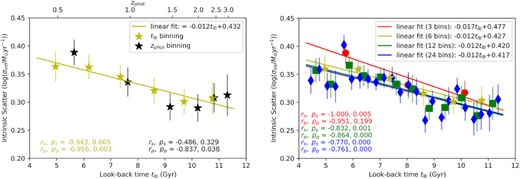
The left-hand panel is intrinsic MS scatter versus zphot and tlb binning with a linear regression fit to the look-back time bins. The yellow star-like scatter points are the tlb binning data. We take the average of the data points in each mass bin, and obtain error bars of intrinsic MS scatter by bootstrap resampling the distribution 100 times based on varying the individual values by their uncertainties and rebinning them. The solid yellow line is the linear fit of intrinsic MS scatter versus tlb. The right-hand panel display the effect of binning number. A total of 12 380 galaxies are regrouped in 3, 6, 12, and 24 bins with red circles, yellow star, green squares, and blue diamonds. In each panel, we show the Spearman and Pearson correlation coefficients (rs and rp) as well as the corresponding p-values (ps, pp) for different binning data.
The intrinsic MS scatter may vary with the adopted Δtlb of each bin. The right-hand panel of Fig. 11 presents the effect of binning the data in different Δtlb widths. The data are binned into 3, 6, 12, and 24 groups (no less than 100 galaxies in each bin) in four different sets with equal tlb widths, where six is our fiducial number of bins. It can be seen that the data in the 12 and 24 bins have a similar distribution statistically relative to our fiducial binning. We find that as the number of bins increases, the normalization (intrinsic MS scatter) slightly decreases. However, the coefficients of the corresponding equations tend to converge somewhere closely below the current linear regression equation (i.e. the yellow line). Even though the decreasing binning time-scale causes more severe fluctuation along the linear regression line, the similarity and high absolute values of rs and rp still demonstrate a strong correlation between intrinsic MS scatter and tlb. On the other hand, this phenomenon also partially explains why redshift binning is not a good approach in this study, especially at high redshifts: a narrower binning time-scale may lead to larger fluctuations in the intrinsic MS scatter. Since there is no significant discrepancy in intrinsic MS scatter for nbin ≥ 6, we expect that these coefficients in linear regression lines approach some values slightly smaller than the current binning one. Hence, we conclude that the binning does not strongly affect the trend of intrinsic MS scatter evolution and we adopt nbin ≥ 6 as the current tlb binning number.
4 DISCUSSION
4.1 Comparison to the halo mass–stellar mass relation
The stochastic events that occurred throughout an SF galaxy’s history, including as galaxy mergers and supernova & AGN feedback, are assumed to be responsible for the inherent MS scatter. The amount of burstiness in SFH, which is probably related to galactic feedback mechanisms, is reflected in the distribution and evolution of intrinsic MS scatter.
In the left-hand panel of Fig. 12, we show the distribution of the intrinsic MS scatter versus M*. We see a minimum intrinsic MS scatter of ∼0.35 dex at M* ∼ 1010.25 M⊙. We see a higher increase of ∼0.1 dex at higher mass (>1011 M⊙) with decreasing look-back time for low redshifts (tlb: 4.9–8.5 Gyr) and a relatively flat relation at higher redshifts (tlb ≳ 9.7 Gyr). In the low-mass end (∼109 M⊙), where the galaxies are mass-incomplete, the intrinsic scatter rises from 0.35 to 0.6 dex. For some of the redshift bins, this type of trend is qualitatively similar to the turnover that occurs in the halo mass–stellar mass (HMSM) relation (see fig. 2 of Wechsler & Tinker (2018)). The shape of the HMSM relation is thought to be a consequence of feedback, with SF feedback reducing the SF efficiency in low-mass galaxies and AGN feedback reducing the SF efficiency in high-mass galaxies, with a turnover at halo mass Mh ∼ 1012 M⊙, which is coincidentally corresponding to the upturn point of M*–σint panel at M* ∼ 1010.25 M⊙ in this study. The intrinsic scatter in the MS is also expected to be linked to feedback, and this may account for similarities in the observed trends with the HMSM relation.
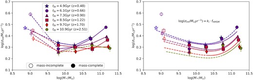
Left-hand panel: the intrinsic MS scatter σ(log (SFR)) versus M* for our six look-back time bins. Solid lines connect the mass-complete data, and dashed lines indicate the mass-incomplete regions. Right-hand panel: we show a fit of our toy model (relation indicated in the panel), based on the halo mass to stellar mass fraction versus stellar mass relation (Behroozi, Conroy & Wechsler 2010) normalized by a constant factor, normalized by a constant factor, relative to our intrinsic MS scatter. Similar to the left, we indicate the mass-complete and mass-incomplete regions with solid and dashed lines, respectively.
Best-fitting values for the constant factor ki at different bins of look-back time for our toy model given by equation (7).
| tlb | ki |
|---|---|
| 4.9 Gyr (z = 0.48) | 0.20 |
| 6.1 Gyr (z = 0.66) | 0.19 |
| 7.3 Gyr (z = 0.90) | 0.17 |
| 8.5 Gyr (z = 1.22) | 0.15 |
| 9.7 Gyr (z = 1.70) | 0.12 |
| 10.9 Gyr (z = 2.51) | 0.10 |
| tlb | ki |
|---|---|
| 4.9 Gyr (z = 0.48) | 0.20 |
| 6.1 Gyr (z = 0.66) | 0.19 |
| 7.3 Gyr (z = 0.90) | 0.17 |
| 8.5 Gyr (z = 1.22) | 0.15 |
| 9.7 Gyr (z = 1.70) | 0.12 |
| 10.9 Gyr (z = 2.51) | 0.10 |
4.2 Comparison to observational studies
We compare our measurements of the intrinsic MS scatter with some previous studies in Fig. 13. Traditionally, a redshift-independent width of MS at either 0.2 or 0.25 dex is founded in observations (Daddi et al. 2007; Noeske et al. 2007; Whitaker et al. 2012; Ciesla et al. 2014; Speagle et al. 2014; Kurczynski et al. 2016), which is lower than our results. In contrast, Kurczynski et al. (2016), Santini et al. (2017), Tacchella et al. (2020), Davies et al. (2022), Shin et al. (2022) report a redshift evolution of intrinsic MS scatter, which spans a wider range from 0.2 to 0.9 dex.
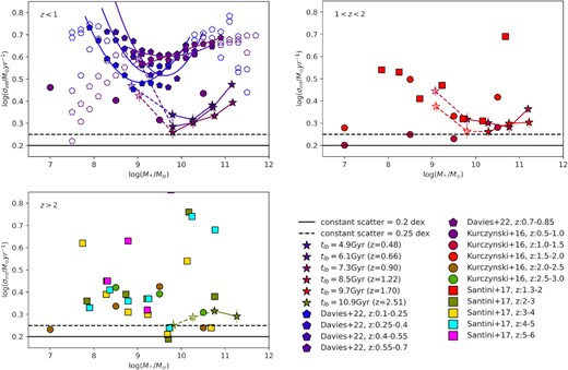
A comparison of our intrinsic MS scatter to previous studies. The first three panels display the distribution of intrinsic MS scatter over M* at zphot < 1, 1 < zphot < 2 and zphot > 2, respectively. The star symbols are the results in this study. The pentagon symbols show the results from Davies et al. (2022), while the curves in the top left-hand panel are polynomial fitting curves to their data. The filled pentagons are the fitting range of Davies et al. (2022). The circles are the results from Kurczynski et al. (2016), while the squares represent the data from Santini et al. (2017). The horizontal dashed line in the bottom indicates a constant intrinsic MS scatter at 0.25 dex (Daddi et al. 2007; Ciesla et al. 2014; Speagle et al. 2014), while the solid line represents a non-evolving scatter at 0.20 dex (Noeske et al. 2007; Whitaker et al. 2012; Pessa et al. 2021). Our data are qualitatively similar to Kurczynski et al. (2016), Davies et al. (2022).
Our data show a similar trend to the ‘U-shaped’ distribution described in Davies et al. (2022). They used the DEVILS survey, containing ∼60 000 galaxies with spectroscopic redshifts ranging from 0.1 to 0.85. In the case of zphot = 0.5, where our samples have redshift overlap, the intrinsic MS scatter trend along the M* is highly consistent with the ‘U-shaped’ distribution, except we have significantly smaller intrinsic MS scatter (0.24–0.40 dex in this study, while ∼0.4–0.8 dex in Davies et al. (2022)). At low-stellar mass, Davies et al. (2022) suggest that the intrinsic MS scatter is driven by stochastic starbursts and stellar feedback events; while the galaxies become more massive and reach intermediate stellar mass (around 1010 M⊙), the galaxies are too massive so that the effect of star formation and galaxy feedback is less significant. In this study, intrinsic MS scatter increases at high stellar mass (log (M*/M⊙) ≳ 10.3), consistent with the ‘U-shaped’ distribution. Davies et al. (2022) conclude that AGN feedback leads to a large scatter at the high-mass end. We note that in our selection, we removed sources with current AGN signatures (see Section 2.1), but that the feedback from previous AGN will still affect the MS scatter over longer time-scales than the AGN duty cycle. As the redshift increases, more data in the low-stellar mass end are identified as mass-incomplete due to IR selection. However, we can still recognize that the intrinsic MS scatter tends to increase when galaxies become more massive for M* > 1010 M⊙. With increasing redshift, we notice that the right half of the ‘U-shaped’ distribution becomes flattered and even decreases at tlb = 10.9 Gyr (zphot = 2.51). This suggests that the star-forming and feedback activity or efficiency for high-mass galaxies in the early universe may differ relative to lower redshifts.
Regarding the higher intrinsic MS scatter in Davies et al. (2022) relative to our results, we think this is due to the following reasons: (1) They do not include photo-z uncertainties in the SED modelling, which results in an underestimate of the measurement uncertainty (on M* and SFR), and hence, an overestimation of the intrinsic MS scatter. (2) They derive galaxy properties for the D10 field of DEVILS (Davies et al. 2018) by using different SED fitting code, PROSPECT (Robotham et al. 2020). Large differences in obtained properties are produced by different derivation techniques applied to various photometric data (see the comparison between PROSPECT and MAGPHYS 3 in Thorne et al. (2021)). (3) They adopt the U–V–J selection rather than sSFR cut so that the samples in Davies et al. (2022) contain low-sSFR galaxies (see the discussion of these two selection criteria in Appendix A). However, in our selection criteria, these galaxies are identified as quenched and removed. The addition of quenched galaxies severely enlarges the MS scatter. As will be shown in Section 4.3 when comparing to simulations, the amplitude of the intrinsic MS scatter is very sensitive to the choice of sSFR cuts. For example, Leja et al. (2022) demonstrate that fixed-sSFR cuts may reduce the inferred MS scatter, particularly at the highest stellar mass. (4) They do not strictly require detection in the IR bands. As discussed in Section 3.1.3, the SED fitting in the absence of IR information results in considerable uncertainty of derived SFR, which may increase the SFR standard deviation and inferred intrinsic MS scatter.
4.3 Comparison to theoretical studies
We first compare to results from the SHARK semi-analytic models (left-hand panel of Fig. 14; Lagos et al. 2018). For SHARK, we select galaxies with stellar masses between 108.25–1011.75 M⊙ within ±1 dex along the MS for each redshifts. We calculate the standard deviations of the median SFRs for selected galaxies and present the results as the dot–dashed lines in Fig. 14. A notable difference from the observational data is that the overall scatter in SHARK is larger than observational data in the mass-complete range, particularly for the highest redshift bin. We find a common trend that the SHARK results follow a similar ‘U-shaped’ distribution at each redshift, though the minimum and maximum points occur at a stellar mass <1010 M⊙ and >1010.75 M⊙, respectively. We suggest that the consistent ‘upturn’ feature in SHARK also indicates the effect of past AGNs for M* ≳ 1010 M⊙. We also observe a flat or decreasing scatter in SHARK for galaxies in the range of M* ≥ 1010.75 M⊙. This occurrence indicates that galaxies in this mass range are shifted below the chosen sSFR limit because AGNs have a more significant impact on them. We also investigate the effect of the sSFR cut on intrinsic MS scatter, and find that the stricter sSFR cut leads to a smaller amplitude of the intrinsic MS scatter. For instance, the intrinsic MS scatter will be reduced by ∼1 dex overall when we pick a selection with a narrower sSFR cut, such as ±0.75 dex along the MS, rather than ±1 dex.
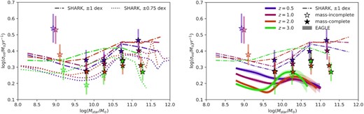
Left-hand panel: we compare our results with SHARK models and show the sensitivity of the intrinsic MS scatter to the chosen boundary of sSFR (i.e. ±1 and ±0.75 dex). The trends in SHARK show rough qualitative agreement with our observational results but with slight differences in the normalization, which is sensitive to the adopted sSFR cut. Right-hand panel: we overlap the results from the SHARK (dot–dashed lines) and EAGLE (solid bands) simulations (Lagos et al. 2018; Matthee & Schaye 2019) with our data. For both panels, we have modified our bins to be consistent with the bins used in Matthee & Schaye (2019). At M* > 109.8 M⊙, where we are mostly mass-complete, we find differing trends between the observational results and the EAGLE simulations, and also note there are large differences in the trends inferred from SHARK and EAGLE. We obtain error bars of intrinsic MS scatter by bootstrap resampling the data by their uncertainties 100 times and remeasuring the intrinsic scatter.
Next, we compare the results with EAGLE hydrodynamical simulations (right-hand panel of Fig. 14; Matthee & Schaye 2019). We redivide the data in redshift binning at zphot = 0.5, 1.0, 2.0, and 3.0 for a proper comparison with fig. 3 in Matthee & Schaye (2019). Matthee & Schaye (2019) adopt SF galaxies with evolved sSFR selection (i.e. log (sSFR/yr−1) = −10.4 at z = 0.5 and increases to −9.4 at z = 3) and measure the scatter from the residuals by using the non-parametric local polynomial regression method. Then they obtain the intrinsic MS scatter by subtracting the observational errors derived by median uncertainties of the observational sample from Chang et al. (2015). The EAGLE results suggest lower intrinsic MS scatter at higher redshift for M* < 109.8 M⊙ and similar intrinsic MS scatter for M* > 109.8 M⊙, with a downward ‘U-shaped’ feature appearing at z = 2 and 3. This shape differs substantially from our findings. Unlike the decreasing trend with stellar mass from simulation, the intrinsic MS scatter in this study decreases initially but increases at the high-mass end. Matthee & Schaye (2019) consider that supermassive black hole growth accounts for the increasing scatter at M* ≈ 109.8 M⊙ at high redshift. However, our results suggest the influence of the feedback mechanism from previous AGNs might be more significant at higher stellar masses (M* ≳ 1010.3 M⊙) at low redshift. The intrinsic MS scatter at each redshift bin is also larger than Matthee & Schaye (2019). We suspect that different physics (e.g. feedback, SF model) adopted in EAGLE give rise to the quantitative difference to our results and from SHARK.
5 CONCLUSIONS
In this paper, using the selection of 12 380 SF galaxies from the COSMOS2020 data base and adopting the MAGPHYS + photo-z SED fitting code, we characterize the intrinsic scatter of galaxy MS over the redshift range 0.5 < z < 3.0.
We find that the intrinsic MS scatter is larger than the measurement uncertainty by a factor of 1.4–2.6 when IR data is available for accurately constraining the dust-obscured star formation (Section 3), with measured MS scatter in the range of 0.26–0.47 dex.
For the COSMOS2020 sample, the inclusion of IR data is the dominant factor (over zphot uncertainty), affecting the accuracy of measuring the scatter on the MS.
Binning the data according to either redshift or look-back time, we find a slightly negative correlation between intrinsic MS scatter and look-back time (equation (6)) but with an upturn at tlb ≳ 10 Gyr.
To connect the intrinsic MS scatter with the feedback mechanism, we present a toy model that uses the Behroozi et al. (2010) SMHM relation (equation (7)), which does a reasonable job of matching the distribution of intrinsic MS scatter over M* and redshift (Fig. 12), although with less agreement at the highest redshifts.
We compare our results to other observational studies of the MS scatter. Differing from a non-evolving, mass-independent scatter, our results are qualitatively similar to the ‘U-shaped’ intrinsic MS scatter distribution with stellar mass and redshifts found in Davies et al. (2022).
We compare the intrinsic MS scatter to some theoretical studies. The consistent upturn trend in SHARK models suggests the agreement of the feedback mechanism from past AGN activity for galaxies with M* > 1010 M⊙. These comparisons highlight the significant influence that sSFR cuts can have on the measured value of the ‘intrinsic’ MS scatter and that particular care needs to be taken with such comparisons. We also find that the behaviour of intrinsic MS scatter diverges significantly between our study and EAGLE simulation.
In the future, the most significant gain in our understanding of the evolution in the MS scatter will come from deeper surveys in rest-frame IR to enable accurate characterization of the MS scatter at both low-stellar masses and higher redshifts, where our current sample is severely limited. There is a weak agreement between observation data and theory in equation (7) for high-z and low-mass cases. In particular, better sampling in these regimes will provide a clear test of whether our toy model linking the MS scatter to the HMSM relation is reasonable. Alternatively, we also plan to explore less-restrictive selection criteria in the IR bands to push our sample to include more low-M* and/or high-z sources from existing surveys.
ACKNOWLEDGEMENTS
The authors appreciate the referee, Antonios Katsianis, who provided valuable and insightful comments on the manuscript. Parts of this research were supported by the Australian Research Council Centre of Excellence for All Sky Astrophysics in 3 Dimensions (ASTRO 3D), through project number CE170100013. We thank the COSMOS team for making the data products that we used in this project. K.G. is supported by the Australian Research Council through the Discovery Early Career Researcher Award (DECRA) Fellowship DE220100766 funded by the Australian Government. We also thank Jorryt Matthee for correspondence regarding his study using the EAGLE survey. This research was conducted on Ngunnawal Indigenous land.
DATA AVAILABILITY
The observational data used in this paper are publicly available through catalog and imaging data releases from the COSMOS survey team (see Section 2.1). Other data products can be made available upon reasonable request to the first author.
Footnotes
We explored adopting a constant cut at log (sSFR/yr−1) = −11, which increases our sample by ∼100 galaxies, but this has a very small difference on our results. We suspect that this phenomenon could be driven by IR-selection, which is described in the next subsection.
This excludes the negative-k correction effect.
We pick MAGPHYS + photo-z in this study because this code can treat redshift as a free parameter and derive the zphot and the corresponding measurement uncertainty.
REFERENCES
APPENDIX A: sSFR SELECTION VERSUS U–V–J CUT
We show a comparison between the conventional U–V–J (in rest-frame) selection from Whitaker et al. (2012) and our adopted sSFR selection (see Fig. A1). Since the sSFR is computed by multiband SED fitting, we expect this technique will be more accurate in excluding quenched galaxies than a colour–colour cut based on U, V, and J bands. We find that 75 per cent of galaxies below our sSFR cut are excluded by the U–V–J cut, so the majority of ‘quenched’ galaxies in our samples are also designated as ‘passive’ in the U–V–J diagram. However, only 5.17 per cent galaxies that were eliminated by U–V–J selection lie below our sSFR cut. Hence, the bulk of galaxies excluded by the colour–colour cut for our sample are SF galaxies; presumably, they are dusty SF galaxies. Therefore, we adopt an sSFR cut rather than U–V–J cut to remove quenched galaxies for our analysis.
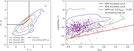
Left-hand panel: U–V–J diagram lot for the 13 071 χ2 selection galaxies. Right-hand panel: in addition to Fig. 4, we show the galaxies removed by U–V–J cut from Whitaker et al. (2012). 64 galaxies are excluded by the sSFR cut, and 929 galaxies are excluded by the U–V–J cut, whereas only 48 of them are marked as quenched galaxies jointly by both selections.
Author notes
ARC DECRA Fellow
