


ABSTRACT
The Event Horizon Telescope (EHT), with ∼20 |$\mu$| as high angular resolution, recently resolved the millimetre image of the suppermassive black hole in the Galaxy, Sagittarius A∗. This opens a new window to study the plasma on horizon scales. The accreting disc probably contains a small fraction of non-thermal electrons and their emissions should contribute to the observed image. We study if such contributions are sufficient to cause structural differences detectable by current and future observational capabilities. We introduce non-thermal electrons in a semi-analytical accretion disc, which considers viscosity-leading heating processes, and adopt a continued hybrid electron energy distribution of thermal distribution and power-law tail. We generate the black hole images and extract the structural features as crescent parameters. We find the existence of non-thermal electron radiation makes the crescent much brighter, slightly larger, moderately thicker, and much more symmetric. When the non-thermal connecting Lorentz factor γc = 65, which is equivalent to the non-thermal electrons accounting for ∼1.5 per cent of the totals, non-thermal effects cause ∼2 per cent size difference at 230 GHz. Comparing with the structural changes caused by other physical factors, including inclination between the system and the observer, black hole spin, and interstellar medium scattering effects, we find that although non-thermal electron radiation takes the most unimportant role at 230 GHz, it becomes more significant at 345 GHz.
1 INTRODUCTION
Recently, high resolution millimetre very long baseline interferometry (mm-VLBI) observations (e.g. the Event Horizon Telescope, EHT, see Event Horizon Telescope Collaboration 2019a, b, c, d, e, f, 2021a, b, 2022a, b, c, d, e, f) and near-infrared astrometry (e.g. GRAVITY, see Gravity Collaboration 2018, 2020a, b) open a new window to study the horizon-scaled astrophysics of the Sagittarius A∗ (Sgr A∗, the suppermassive black hole candidate in the Galactic Centre). The structure of the black hole image at (sub) millimetre wavelengths becomes detectable and can be used to quantitatively study the physical properties of Sgr A∗, including the space–time, the magnetic field, the dynamics of the surrounding plasma, and the radiation.
For radiation, the detected radio waves are emitted from the horizon scale emission region, through the synchrotron radiation mechanism (Yuan & Narayan 2014). Then they bend by the curved space–time in the vicinity of the black hole and finally make up a ring-like bright structure around a dark shadow (Falcke, Melia & Agol 2000). Therefore, the magnetic field structure, the electron properties, and the space–time are all important in modelling the related radiation. Here we focus on the electrons. Suppose all the electrons in the accretion flows are under complete collision, the electrons are in the thermal state. However if some incomplete collision processes exist (e.g. reconnections, shocks), some electrons might be accelerated into higher energy states and become non-thermal.
Non-thermal electrons are used to explain some observations, for example, adding 1.5 per cent non-thermal electrons into the thermal electrons can explain the spectrum at low frequency radio band, as well as the X-ray flares (Yuan, Quataert & Narayan 2003). It is also suggested that non-thermal electrons will enlarge the size of Sgr A∗, especially at low frequency (Özel, Psaltis & Narayan 2000). Recently, non-thermal electrons are used to explain new observations such as the Sgr A∗ near-infrared centroid movement (Petersen & Gammie 2020), multiwavelengths flares (Ball et al. 2016; Chatterjee et al. 2021; GRAVITY Collaboration 2021), and polarimetry (Mao & Wang 2018). As for black hole images, the ring brightness, size, width, and asymmetry are expected to better discriminate the non-thermal electron radiation from the other effects.
Event Horizon Telescope Collaboration (2022e) considered non-thermal electron radiation as one of the physical inputs to interpret the EHT 2017 data at 230 GHz and found that the result is insensitive to whether use non-thermal electron distribution function (eDF) in their radiation model (consistent with some theoretical expectations that the non-thermal effects are negligible, e.g. Chael, Narayan & Sadowski 2017; Mao, Dexter & Quataert 2017). In their works, the non-thermal electrons are mainly introduced in and near the outflow regions, and the results also depend on the electron temperature, which is controlled by a thermodynamical parameter in the relation between the electron temperature and the proton temperature (e.g. Mościbrodzka, Falcke & Shiokawa 2016; Mizuno et al. 2021). This parameter indirectly reveals the physics of the two-tempered accreting plasma (It is generally believed that the electron temperature is much lower than the proton temperature to explain the extremely low bolometric luminosity of Sgr A∗, Lbol ∼ 2 × 10⁻⁹ LEdd; see e.g. Yuan & Narayan 2014).
In this work, we reconsider the impact of the non-thermal electron radiation on the millimetre black hole image structures. First, we introduce the non-thermal electrons globally into the accretion disc, not the jet/outflow region. This is a reasonable choice, since there is no observational conclusion of whether the emissions from the jet region are significant, and the first Sgr A∗ horizon scale image resolved by EHT also do not see jet (Event Horizon Telescope Collaboration 2022a). Secondly, we describe the plasma dynamics using a semi-analytical model by Huang et al. (2009a); Huang, Takahashi & Shen (2009b; here after call the model H09), where the electron temperature is defined by Liu et al. (2007), considering turbulence heating and radiation cooling. There is therefore no need to introduce a free parameter to ‘post-print’ electron temperature, which simplifies the radiation model.
Additionally, we extend the analysis from 230 GHz to 345 GHz. The next generation EHT will be improved to 345 GHz (see e.g. Doeleman et al. 2019; Johnson et al. 2019; Raymond et al. 2021). The higher frequency will not only provide higher resolution, but also reveal the frequency dependent properties in the black hole image. The combination of the current 230 GHz image and the future 345 GHz image is promising in breaking the degeneracy of the effects caused by the non-thermal electron radiation and other physical factors, such as the black hole spin and the interstellar medium scattering.
This paper is written in the following structures. Section 2 shows the non-thermal electron radiation model, which contains a continued hybrid eDF of a thermal distribution with a power-law tail. Section 3 shows the method to generate black hole images, containing the dynamical model, the radiation model, and the scattering model. We also introduce the method of extracting the crescent structural features from the image domain in this section. In Section 4, we show the results of non-thermal images, compare the crescent parameters with those extracted from the images of different inclinations, spin and with/without scattering effects, and rank the importance of each physical factors at 230 GHz and 345 GHz. Finally, conclusions and discussions are given in Section 5.
2 RADIATION MODEL
There are many different ways to build an eDF. The most strict and reasonable way is using particle-in-cell (PIC) simulation with particle acceleration mechanisms (e.g. Lynn et al. 2014; Werner et al. 2018; Comisso & Sironi 2019; Sironi, Rowan & Narayan 2021) to compute the local eDF at each grid of emission region. However it is too computationally expansive to realize, so instead, using a simple function to be non-thermal eDF is a more feasible and generally adopted way. For example, the non-thermal eDF can be expressed as a hybrid function of thermal distribution and power-law tail (e.g. Özel et al. 2000; Yuan et al. 2003; Ball et al. 2016; Chael et al. 2017; Chatterjee et al. 2021; Event Horizon Telescope Collaboration 2021b, 2022e), kappa distribution (e.g. Pandya et al. 2016, 2018; Davelaar et al. 2019; Event Horizon Telescope Collaboration 2022e), and multithermal distributions (Mao et al. 2017).
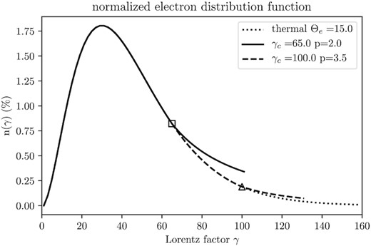
Examples of hybrid normalized eDFs containing a part of Maxwell distribution (thermal electrons) at the low energy region and a power-law tail (non-thermal electrons) at the high energy region. The dimensionless electron temperature is Θe = 15. We show three cases: the pure thermal eDF (dotted line), the non-thermal eDF with γc = 65 and p = 2.0 (solid line), as well as the non-thermal eDF with γc = 100 and p = 3.5 (dashed line), where the connecting point γc = 65 is marked by a square and γc = 100 is marked by a triangle.
By adopting the eDF of equation (2), the emissivety and the absorption in equation (1) become |$j_\nu =j_\nu ^{(1)}+j_\nu ^{(2)}$| and |$\alpha _\nu =\alpha _\nu ^{(1)}+\alpha _\nu ^{(2)}$|, where the upper script (1) and (2) refer to the thermal part and the non-thermal part. See equations (B6) to (B8) and equations (B11) to (B13) in the Appendix B.
We note that γc is the only free parameter in our non-thermal electron radiation model. When γc is small, the proportion of non-thermal electrons is large. γc is independent to Θe, which is determined by the accretion flow model.
3 BLACK HOLE IMAGE GENERATION AND FEATURE EXTRACTION
The radiation model introduced in Section 2 is numerically realized by ray-tracing method (see Section 3.2), which traces the light rays bending in the curved space–time around the black hole, and the corresponding magnetic field and plasma properties at each emitting point come from the dynamical model (see Section 3.1). We also use a scattering model (see Section 3.3) to describe the propagation of the radio waves through the interstellar medium in the Galaxy. We generate millimetre black hole images and extract their structural features (see Section 3.4).
3.1 Dynamical model: semi-analytical model H09
Multiwavelengths observations of Sgr A∗ have shown that it is a hot but quite dim source. This phenomenon can be explained by a geometrically thick but optically thin accretion disc, such as advection-dominated accretion flows (ADAFs; e.g. Narayan & Yi 1994; Mościbrodzka et al. 2009). The main idea of these models is to introduce a mechanism which is efficient in heating the accretion flow but inefficient in radiation. Thus, this kind of models is also called radiatively inefficient accretion flow (RIAF). We refer to Yuan & Narayan (2014) for more details.
There are two kinds of approaches to model the plasma dynamics: one is the semi-analytical approach (e.g. Huang et al. 2009a; Huang et al. 2009b; Broderick et al. 2011, 2016; Pu, Akiyama & Asada 2016; Pu & Broderick 2018); the other one is general-relativistic magnetohydrodynamical (GRMHD) simulation (e.g. Noble et al. 2007; Mościbrodzka et al. 2009; Mościbrodzka et al. 2016; Porth et al. 2019; Mizuno et al. 2021). We choose a semi-analytical approach in order to get a concrete electron temperature by solving the electron temperature and proton temperature simultaneously from the MHD equation, which is out of computational feasibility for most of the GRMHD simulations.
H09, the semi-analytical model applied in this work, well describes the electron temperature by assuming the electrons are heated mainly by the viscosity, which is generated by the plasma fluctuations (based on the work by Liu et al. 2007). Two other processes, the energy exchange between the electrons and protons, and the radiative cooling effects are also considered. In the model, the density distribution and the velocity field are obtained by solving the basic equations of the general relativistic accretion flow. The magnetic field is initialized in a vertical structure. After being sheared by the accretion flow, it is finally in a configuration which is parallel to the velocity filed. H09 accretion disc is defined by four parameters: the spin of black hole a*, the ratio of the magnetic field energy density to the gas pressure βp, dimensionless constant for electron heating rate C1, constant mass accretion rate |$\dot{M}$|. It should be noted that the mass accretion rate decreases with decreasing radius, due to the existence of strong winds in the accretion flow (Yuan, Bu & Wu 2012; Yuan et al. 2015). But considering the wind is weak at the inner region (r < 30rg, see Yang et al. 2021), where the radiation of interest mainly comes from, we treat the mass accretion rate as a constant. We take the models with a* = 0, 0.5, 0.9, 0.95 in this work, while other three parameters are chosen carefully in order to make sure the flux density of Sgr A∗ at 230 GHz is in the range of ∼1 to several Jy with any alternative inclination. Exploring the whole dynamical model parameter space is beyond the scope of this work.
3.2 Ray-tracing scheme: ipole
We use the ray-tracing scheme ipole1 developed by Mościbrodzka & Gammie (2018) to trace the light emitted from the H09 accretion disc, bending in the Kerr space–time and captured by a camera at 1000 rg far from the black hole. We integrate the radiative transfer equation (1) along each light and finally get the black hole image. It is capable of generating images of any inclination. ipole is one of the adopted ray-tracing codes in the theoretical works by EHT collaboration (Event Horizon Telescope Collaboration 2019e, 2021b, 2022a) and have been well compared with other ray-tracing codes by Gold et al. (2020).
3.3 Scattering: isotropic Gaussian thin screen
At centimetre wavelengths, scattering effects appear as a Gaussian broadening of the source, proportional to the square of the wavelength. At (sub)millimetre wavelengths, diffractive scattering blurs the image by an anisotropic Gaussian, and refractive scattering causes refractive noise on the image. In this work, we focus on ensemble-averaged scattering model, which means that the averaging time is longer than the typical decorrelation time-scale for refractive noise, i.e. days to weeks (see Johnson 2016). Therefore the refractive noise is smoothed, and the scattering is described by an anisotropic Gaussian blur. We use Gaussian parameters measured by Johnson et al. (2018): the major axis size θmaj = 1.38, minor axis size θmin = 0.703, position angle ϕPA = 81.9° (reference to the source at 1 cm wavelengths). The more complicated scattering models involving refractive scattering effects can be found in the works by e.g. Johnson et al. (2018), Zhu, Johnson & Narayan (2019), Issaoun et al. (2019), Issaoun et al. (2021), which are beyond the scope of this work.
3.4 Feature extraction: parametrize the image into crescent parameters
Inspired by the ring parameter extraction in Event Horizon Telescope Collaboration et al. (2019d), we use crescent model to extract the structural features of a image. A crescent is formed by a large uniformed brightness disc with subtracting a small disc from it, which is described by five parameters: the total intensity Itot, the overall size R, the relative thickness ψ, the degree of symmetry τ, and the orientation ϕ, following Kamruddin & Dexter (2013). Extract the crescent parameters from the image domain contain three steps:
Find the crescent centre
The crescent centre (x0, y0) is defined as the centre of the large disc (where x0, y0 are described in the Cartesian coordinate of the image), and we find it by roughly fitting the image with a infinite-thin-ring. To do the fitting, first, we take a polar coordinate with the origin at an arbitrary (x0, y0), and then for each position angle θi, there is a peak radius rpk, i, which is corresponding to the peak of the 1D intensity profile |$I(r)|_{\theta _i}$|. We change the (x0, y0) and finally find the best fit when the peak radius set {rpk, i} has the minimum standard deviation.
Find the size of two disks and locate the small disc
We take the crescent centre determined by step (i) as the origin of the polar coordinate, and for each θi, we fit |$I(r)|_{\theta _i}$| with Gaussian components to get the locations of their full width at half maximum, where the one closer to the origin is written as rS, i, and the outer one is written as rL, i. We fit the point set {(rL, i, θi)} to a circle with radius RL at the crescent centre, while fit {(rS, i, θi)} to a smaller circle radius RS, and its centre is at (a, b), where (a, b) is described in Cartesian coordinate respect to the crescent centre. We take the best-fitting RL, RS, and (a, b) as the large disc radius, small disc radius, and small disc centre of the crescent model, respectively. Fig. 2 shows an example of feature extraction, where the right-hand panel shows the 1D intensity profile at θ = 0°, 45°, 90°.
Calculate the crescent parameters
The crescent parameters are defined by Kamruddin & Dexter (2013):(7)$$\begin{eqnarray*} \rm {intensity} && I_{\rm tot}=\sum _{i,j} I_{i,j}, \end{eqnarray*}$$(8)$$\begin{eqnarray*} \rm {overall\ size} && R=R_L, \end{eqnarray*}$$(9)$$\begin{eqnarray*} \rm {relative\ thickness} && \psi =1-\frac{R_S}{R_L}, \end{eqnarray*}$$The left-hand panel of Fig. 2 shows the best-fitting crescent and the corresponding parameters.(10)$$\begin{eqnarray*} \rm {degree\ of\ symmetry} && \tau =1-\frac{\sqrt{a^2+b^2}}{R_L-R_S}. \end{eqnarray*}$$
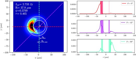
This draft shows how to extract crescent features from a given image. The left-hand panel is the model image of i = 45°, a* = 0.5, thermal model, without scattering effects. A large circle with radius RL and a small circle with radius RS are drawn with white colour in the image. The red, magenta, and cyan dashed lines refer to the angular direction of θ = 0°, 45°, 90°, and the 1D intensity profile at each direction are plotted with the same colour in the right-hand panel. The shaded area in the right-hand panel refers to the bright part of the crescent, based on the full width at half maximum of the best-fit Gaussian distributions of the profile. The crescent parameters are in the legend in the upper left corner.
4 RESULTS
4.1 Non-thermal images
Following Section 2 and Section 3, we calculate the black hole images of non-thermal models at 230 GHz (see Fig. 3 top row), and their differences from the thermal model (Fig. 3 bottom row). For the case of γc = 80, it shows almost no difference, while γc = 50 shows more differences.
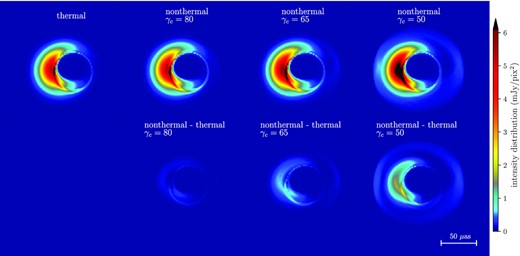
Top row: Black hole images of thermal electron radiation model and the non-thermal electron radiation model with power-law connecting energy γc =80, 65, 50. Bottom row: The remaining intensity distribution of the non-thermal model images after removal of the intensity distribution of the thermal image (the top left). All the images use the same colour bar as shown on the right. The observing frequency is 230 GHz, inclination is i = 45°, spin a* = 0.5, without considering scattering effects.
To quantify the difference, we extract the structural features of each black hole image with four crescent parameters, i.e. intensity Itot, overall size RL, relative thickness ψ and degree of symmetry τ, through the parametrizing method introduced in Section 3.4. We plot the crescent parameters with varying γc in Fig. 4. We see that the four crescent parameters of the non-thermal models are all larger than the corresponding parameters of the thermal model, and their differences become small when γc is large. For a small γc, e.g. γc ∼ 50, the non-thermal electron radiation increase the intensity from ∼2.7 Jy predicted by the thermal model to ∼4 Jy, enlarge the overall size from |$\sim 38\ \mu$|as to |$\sim 42\ \mu$|as,2 make it thicker (relative thickness from ∼0.38 to ∼0.44), and much more symmetric (degree of symmetry from ∼0.45 to ∼0.75). We also find that the overall size R is only sensitive to small γc, if γc ≳ 70, R becomes identical to the value of thermal model.
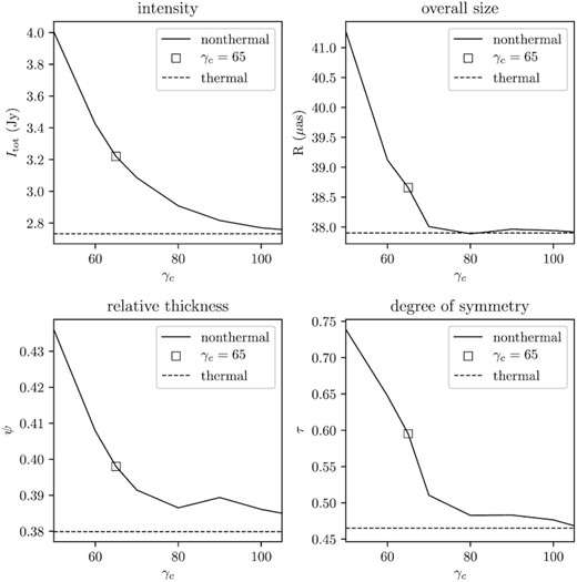
The four crescent parameters extracted from the corresponding black hole images with changing γc (solid lines), compared with the corresponding values of thermal model (dashed lines). The square maker shows the characterized non-thermal model γc = 65, which means that the non-thermal electrons account for ∼1.5 per cent of the totals. The observing frequency is 230 GHz, inclination is i = 45°, spin a* = 0.5, without considering scattering effects.
The four crescent parameters are all enlarged when γc is small (small γc means large non-thermal electron fraction, and their relation is shown in Fig. A1, right-hand panel), because, on the one hand, the outer emission regions that are too dim to be detected in the thermal model case, are now lighted by the radiation emitted from the non-thermal electron. On the other hand, the size and shape of the black hole shadow, which is determined by space–time, is not affected by the non-thermal model. The removed inner disc remains same, while the outer disc becomes larger and brighter, making the four crescent parameters larger.
Additionally, we highlight the non-thermal model with a characterized value γc = 65 (square markers) in Fig. 4, which is consistent with the |$\sim 1.5{{\ \rm per\ cent}}$| non-thermal electron fraction suggested by Yuan et al. (2003). Section A shows the relation between γc and the non-thermal electron fraction. We take the model of γc = 65 as the representative non-thermal model in the later analysis.
4.2 Compare with other physical factors: inclination, spin, scattering effects
In this section, we quantitatively compare the impact on the black hole image structures caused by the non-thermal electron radiation with other physical factors: the inclination, the spin, as well as the scattering effects. Following Section 4.1, we analyse the differences caused by each factor through comparing their crescent parameters. The non-thermal model is chosen as the model of γc = 65.
We calculate the 230 GHz image and the 345 GHz image with inclination i ∈ (0°, 90°), spin a* = 0, 0.5, 0.9, 0.95, with/without scattering and with/without non-thermal electron radiation. Then we extract the corresponding crescent parameters from those images (see Fig. C1).
Here we focus on models with i = 5°, 45°, 90°, a* = 0, 0.5, 0.9, 0.95, with/without scattering and with/without non-thermal electron radiation. Their crescent parameters are listed in Table 1. The corresponding images at 230 GHz and 345 GHz are shown in Figs 5 and 6.
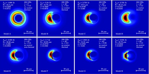
Images of 8 selected models at 230 GHz, with different inclination, spin, with/without scattering and with/without non-thermal electron radiation.
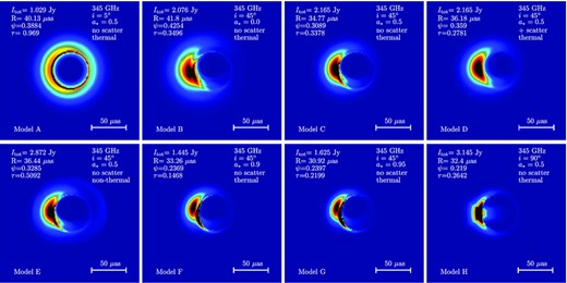
Same as Fig. 5, but at 345 GHz.
The extracted crescent parameters of the black hole images of different models at 230 GHz and 345 GHz.
| model | i(°) | a* | scat. | nont. | Itot (Jy) | R (|$\mu$|as) | ψ | τ | ||||
|---|---|---|---|---|---|---|---|---|---|---|---|---|
| 230 GHz | 345 GHz | 230 GHz | 345 GHz | 230 GHz | 345 GHz | 230 GHz | 345 GHz | |||||
| Mod A | 5 | 0.5 | 1.686 | 1.029 | 42.3 | 40.13 | 0.4205 | 0.3884 | 0.9711 | 0.969 | ||
| Mod B | 45 | 0 | 3.24 | 2.076 | 44.76 | 41.8 | 0.4889 | 0.4254 | 0.4679 | 0.3496 | ||
| Mod C | 45 | 0.5 | 2.733 | 2.165 | 37.9 | 34.77 | 0.3799 | 0.3089 | 0.465 | 0.3378 | ||
| Mod D | 45 | 0.5 | √ | 2.733 | 2.165 | 40.13 | 36.18 | 0.4751 | 0.359 | 0.3535 | 0.2781 | |
| Mod E | 45 | 0.5 | √ | 3.222 | 2.872 | 38.66 | 36.44 | 0.398 | 0.3285 | 0.5952 | 0.5092 | |
| Mod F | 45 | 0.9 | 1.7 | 1.445 | 32.92 | 33.26 | 0.2772 | 0.2369 | 0.1922 | 0.1468 | ||
| Mod G | 45 | 0.95 | 1.642 | 1.625 | 31.91 | 30.92 | 0.2705 | 0.2397 | 0.221 | 0.2199 | ||
| Mod H | 90 | 0.5 | 2.844 | 3.145 | 33.79 | 32.4 | 0.2558 | 0.219 | 0.2217 | 0.2642 | ||
The structural changes of the images due to inclination, spin, scattering effects, and the observing frequency are summarized as follows:
Inclination: The face-on-system Model A (i = 5°) shows ring-like structures with lower intensity, larger size, relatively larger thickness, and high symmetry. Model C(i = 45°) shows highly asymmetric crescent structures and the four crescent parameters changes a lot comparing to Model A, due to the Doppler beaming effects of the rotating plasma. For edge-on Model H (i = 90°), we find the direct emission from the disc in front of the black hole shadow. We can also see a more compact ring (smaller R, ϕ and τ), because the strong gravitational lensing effect takes a more important role and concentrates the lights near the photon sphere.
Spin: Model F and G refer to fast-rotating black hole (a* = 0.9, 0.95). Their images show a much more compact and moderately fainter ring, compared with the image of non-rotating black hole Model B (a* = 0). It is because the high spin systems have smaller innermost stable circular orbits (ISCO), which plays the role of the inner cut-off of the accreting plasma. And when the cut-off is closer to the centre, the corresponding ultra relativistic plasma near the ISCO have higher energy, which leads to a more concentrate emission distribution.
Scattering effects: The model D is same as the model C but considering scattering effects. Scattering effects make the ring larger, thicker, and more symmetric, which is similar to the effects caused by the non-thermal electron radiation (see model E). But scattering effects do not change the intensity, while non-thermal model increases the intensity.
Frequency: Comparing Fig. 5 with Fig. 6, we find the rings for each model are generally more compact at 345 GHz than 230 GHz. Scattering effects significantly decrease at 345 GHz.
4.3 Importance of the non-thermal electron radiation at 230/345 GHz
To rank the importance of each physical factors, we compare the maximum fractional variations in the crescent parameters, which is relative to the fiducial model (model C, i = 45°, a* = 0.5, without scattering effects, without non-thermal electron radiation). The results are displayed in Table 2 and Fig. 7.
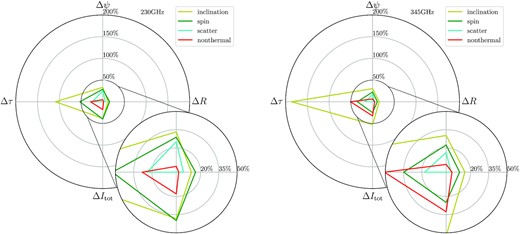
Radar plot of the maximum fractional variations of the crescent parameters due to inclination (olive), spin(green), scattering(cyan), non-thermal electron radiation (red), relative to the fiducial model (model C, i = 45°, a* = 0.5, without scattering effects, without non-thermal electron radiation). The left-hand panel is for 230 GHz, the right-hand panel is for 345 GHz.
The maximum fractional variations of the crescent parameters relative to those extracted from the fiducial model (model C, i = 45°, a* = 0.5, without scattering effects, without non-thermal electron radiation).
| ΔItot (%) | ΔR (%) | Δψ (%) | Δτ (%) | |||||
|---|---|---|---|---|---|---|---|---|
| 230 GHz | 345 GHz | 230 GHz | 345 GHz | 230 GHz | 345 GHz | 230 GHz | 345 GHz | |
| Inclination | 38.29 | 52.47 | 12.37 | 15.41 | 33.23 | 30.2 | 108.8 | 186.9 |
| Spin | 39.92 | 24.94 | 15.81 | 11.07 | 28.8 | 22.39 | 52.47 | 34.9 |
| Scatter | 0 | 0 | 5.882 | 4.044 | 25.08 | 16.23 | 23.98 | 17.67 |
| Non-thermal electrons | 17.9 | 32.63 | 2.001 | 4.806 | 4.767 | 6.351 | 27.99 | 50.75 |
We find that, at 230 GHz, generally speaking, the rank of the importance is: inclination ≳ spin > scattering ∼ non-thermal. The variations of crescent parameters caused by the non-thermal model are |$\Delta I_{\rm tot}\simeq 17.9{{\ \rm per\ cent}}$|, |$\Delta R\simeq 2.0{{\ \rm per\ cent}}$|, |$\Delta \phi \simeq 4.8{{\ \rm per\ cent}}$|, and the most sensitive one |$\Delta \tau \simeq 28.0{{\ \rm per\ cent}}$|. The non-thermal electron radiation is the most unimportant factor compared to others, except that the ΔItot and Δτ due to the non-thermal model are larger than those due to the scattering effects. However, at 345 GHz, the rank becomes: inclination > non-thermal ≳ spin > scattering. The non-thermal variations of the crescent parameters are |$\Delta I_{\rm tot}\simeq 32.6{{\ \rm per\ cent}}$| (rank 2nd), |$\Delta R\simeq 4.8{{\ \rm per\ cent}}$| (rank 3rd), |$\Delta \phi \simeq 6.4{{\ \rm per\ cent}}$| (rank 4th), and |$\Delta \tau \simeq 50.8{{\ \rm per\ cent}}$| (rank 2nd).
Comparing the result at 230 GHz with those at 345 GHz, we summarize: first, the structural difference due to the non-thermal model is enhanced at higher frequency. It is because the emission region at 345 GHz is more concentrated in the inner region, where the non-thermal electron radiation is enhanced by gravitational lensing and Doppler boosting. Secondly, the non-thermal electron radiation is the most unimportant physical factor at 230 GHz, while it becomes relatively more important at 345 GHz, due to the enhancement by itself as well as the weakening of scattering effects and spin effects. Since we only consider the Gaussian blur effects in the scattering model, the value is proportional to the square of the observing wavelengths, which makes the scattering effects weaker at 345 GHz. The weakening impact of the spin at 345 GHz is the result of the combined effects of the accretion rate, magnetic field properties, and the electron heating process. Finally, between 230 GHz and 345 GHz, the enhancements of the importance of the non-thermal model for the four crescent parameters are not equal: the intensity and the symmetry are significantly increased, while the size and the thickness are only moderately increased.
5 CONCLUSIONS AND DISCUSSIONS
We study the impact of non-thermal electron radiation on the horizon-scaled structures of Sgr A∗. The non-thermal electrons are introduced globally into the accretion disc, which is defined by the semi-analytical dynamical model H09. Their radiation is described by adopting a continued hybrid eDF of a part of thermal distribution with a non-thermal power-law tail, controlled by the connecting point energy γc. We calculate the black hole images at 230 GHz and 345 GHz through ray-tracing scheme, and extract the structural features to four crescent parameters: the intensity Itot, the overall size R, the relative thickness ϕ and the degree of symmetry τ, and then use these crescent parameters to quantify the impact of non-thermal electron radiation. For comparison, we do the same for other physical factors, including the inclination, the spin and the scattering effects. We find that:
the existence of non-thermal electron radiation makes the crescent much brighter, slightly larger, moderately thicker, and much more symmetric. Such structural changes are more evident with smaller γc, when γc ≳ 100, they can be neglected.
For the case of γc = 65 (∼1.5 per cent of total electrons are non-thermal), the non-thermal model results in a size difference of ∼2 per cent at 230 GHz, which is twice smaller than the uncertainty of ring size measurement by EHT. But at 345 GHz, the size difference increases to ∼5 per cent, which makes it detectable.
The non-thermal electron radiation is the most unimportant factor at 230 GHz, which is comparable to the scattering effects. However it becomes relatively significant at 345 GHz, much more evident than the scattering effects, comparable to the spin and only less important than the inclination.
Our 230 GHz result is very consistent with the theoretical interpretation of EHT 2017 observation of Sgr A∗ (Event Horizon Telescope Collaboration 2022e) that non-thermal electron radiation is unimportant under the current observational capability. Comparing with the ring fitting results of the EHT data (Event Horizon Telescope Collaboration 2022c), i.e. |$51.8\pm 2.3\ \mu$|as diameter with ∼30 per cent–50 per cent fractional width, both of the ring structures of the thermal/non-thermal model images in our work are within this range. The size difference (∼2 per cent) and thickness difference (∼5 per cent) due to the non-thermal model are less than the uncertainty of the EHT ring fitting results (∼4 per cent for size and ∼20 per cent for thickness).
The future sub-millimetre VLBI observations are very promising in successfully detecting the horizon-scaled structures containing non-negligible non-thermal electron radiation effects. The next generation EHT will provide a factor of two higher angular resolution (from 20 |$\mu$| as to 10 |$\mu$| as, see Doeleman et al. 2019) at 345 GHz, and the ∼5 per cent size difference and the ∼6 per cent thickness difference by the non-thermal model are sufficiently large under such resolution. The asymmetry may also be measured with higher quality data in the future. Our work suggest that the non-thermal model will cause ∼50 per cent asymmetry difference at 345 GHz.
In the more distant future, space VLBI will extend the baseline to a length far more than the Earth's diameter, and can reach higher frequency since it can avoid atmospheric effects. Roelofs et al. (2019), Palumbo et al. (2019), Johnson et al. (2020), Andrianov et al. (2021), Likhachev et al. (2022) show such ideas and Johnson et al. (2021) observed Sgr A∗ by space VLBI at 1.35 cm. Chael, Johnson & Lupsasca (2021) suggest that if the angular resolution can be better than |$1\mu$| as and the dynamic range is sufficiently high, the detection and measurement of inner shadow, or called lensed horizon, is possible. The relative location and the shape of the inner shadow is very sensitive to the inclination, and can be also used to constrain the spin. In addition, the sub-rings, which are the higher order gravitation lensing rings hiding in the unresolved photon ring, may also be used to precisely estimate the space–time related parameter, such as the spin (see Johnson et al. 2020). Therefore, because of the lambda-square-scattering effects become very weak at high frequencies, and the inclination and the spin can be constrained through other observables, the non-thermal electron radiation effects may become distinguishable by the space VLBI.
Our work shows that the the flux density of Sgr A∗ increases when the non-thermal model is considered, but this conclusion is based on the time-independent accretion disc. However the flux density of Sgr A∗ varies frequently, fluctuating ∼1 Jy around 2–3 Jy within several hours at 230 GHz (Wielgus et al. 2022). The ∼18 per cent intensity difference due to the non-thermal model is smaller than its time variation.
Previous theoretical works predicting the impact of non-thermal electron radiations on millimetre image structures have only focused on 230 GHz. Chael et al. (2017) found that non-thermal image is unchanged when compared to the thermal image, which is consistent with our model’s prediction for large γc. Mao et al. (2017) found that the non-thermal model predicts a larger and more diffuse image. This diffusion effect is not seen in our work, because the accretion flow model used in our work does not contain filament structures as theirs.
Our results depend on the way of introducing the non-thermal electrons. At 230 GHz, the results of introducing non-thermal electrons globally in the accretion disc and introducing the non-thermal electrons mainly in the outflow region (Event Horizon Telescope Collaboration 2022e) are very consistent. It is not clear if the outflow-region non-thermal model effects also become more evident at 345 GHz or at even higher frequency. If the answer is not, then such two kind of non-thermal models may provide different predictions towards future observations.
ACKNOWLEDGEMENTS
We thank Prof. Yuan, F. of the Shanghai Astronomical Observatory, the internal referee of the Event Horizon Telescope Collaboration and the anonymous referee for helpful comments. This work was financially supported by the China Postdoctoral Science Foundation fellowship (2020M671266); Shanghai Super Postdoctoral Program; Max Planck Partner Group of the MPG and the CAS; the Key Program of the National Natural Science Foundation of China (grant number 11933007); the Key Research Program of Frontier Sciences, CAS (grant number ZDBS-LY-SLH011, QYZDJ-SSW-SLH057) and the Shanghai Pilot Program for Basic Research - CAS, Shanghai Branch (JCYJ-SHFY-2022-013).
DATA AVAILABILITY
The data generated in this work will be shared on reasonable request to the corresponding author.
Footnotes
The ring diameter of Sgr A∗ measured by EHT is 51.8 ± 2.3 |$\mu$| as, and the fractional width is ∼30–50 (see table 1 in Event Horizon Telescope Collaboration 2022a), which corresponds to a crescent overall size R in the range of ∼39.6–54.1 |$\mu$| as. Considering that our model images are not convoluted with the 20 |$\mu$| as EHT resolution, we allow R of the model images to be a bit smaller than |$39.6\ \mu$| as, and only let 54.1 |$\mu$| as as the upper constraint.
REFERENCES
APPENDIX A: PARAMETER LIMITATIONS OF THE RADIATION MODEL
The non-thermal radiation model shown in Section 2 has two parameters: the connecting Lorentz factor γc and the index p. We consider the following three constraints of the parameter space:
We compare the emissivity equation (B6) with the approximate emissivity of the thermal model (given by Mahadevan, Narayan & Yi 1996), and find that when γc/Θe ≳ 10, their difference is less than |$\mathcal {O}(10^{-2})$|, which means that we can use thermal eDF instead of non-thermal eDF. In H09, the majority part of the accretion disc has the electron temperature Θe ≲ 10, so if γc ≳ 100, the non-thermal electron radiation contribute very little to the image.
- The eDF should be thermal-dominated and the non-thermal part should not be too large. We let the connecting point γc larger than the peak position γpk of the thermal distribution. γpk is defined by |$[\partial n_{\rm th}(\gamma)/\partial \gamma ]|_{\gamma _{\rm pk}}=0$|, which is equivalent toWhen γpk is larger than 1, the numerical solution is(A1)$$\begin{eqnarray*} \left(2\gamma ^{-1}+\gamma ^{-3}\beta ^{-2}-\Theta _e^{-1}\right)\big {|}_{\gamma _{\rm pk}}=0. \end{eqnarray*}$$Considering γc, min = γpk, the above equation becomes equation (5).(A2)$$\begin{eqnarray*} \gamma _{\rm pk}=2\Theta _e+0.25\Theta _e^{-1}. \end{eqnarray*}$$
In order to let equation (4) have real solution, there is an inequality depending on the dimensionless electron temperature Θe, p, and γc. We let Θe and γc free, and solve the upper limit pmax for each Θe and γc, and then plot the results in the left-hand panel of Fig. A1. It seems that pmax depends on γc/Θe, and this relation changes when Θe is small. So fitting the data in the plot, we find a numerical approximation of pmax, which is equation (6).
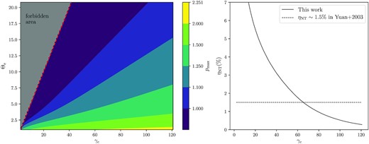
Left: the possible parameter space of the connecting point γc and power-law index p with different electron temperature Θe. The colour represents the max value of p as defined by equation (6). The red dashed line shows the minimum γc which is defined by equation (5). The forbidden area coloured by grey is where |$\gamma _c\lt \gamma _{c,\rm min}$|. Right: Averaged fraction of the non-thermal electrons in the accretion disc ηNT with different γc (solid line). Comparing with the suggested value |$\eta _{\rm NT}\sim 1.5{{\ \rm per\ cent}}$| in the work of Yuan et al. (2003) (dashed line), we find that γc is ∼65.
Additionally, when p = pmax is fixed, we obtain the relation between our model parameter γc and the fractional number of the non-thermal electrons ηNT by integrating the non-thermal eDF. Since different emission regions in the accretion disc have different electron temperatures, we average the results of each region. We plot the ηNT with different γc in the right-hand panel of Fig. A1. Then we read that when |$\eta _{\rm NT}\sim 1.5{{\ \rm per\ cent}}$|, the corresponding γc is about 65.
APPENDIX B: RADIATIVE TRANSFER
The double integrals in |$j_\nu ^{(2)}$| and |$\alpha _\nu ^{(2)}$| brings difficulties in directly computing the radiative transfer coefficients. Some works adopt approximations to replace the exact solution, (e.g. Huang & Shcherbakov 2011; Dexter 2016; Pandya et al. 2018). Our solution is searching the interpolation from a number list which have saved the results of the double integrals with a grid of different p and the lower and upper limits of each integral. The precision of the interpolated number is ≲ 10−3, which is enough for this work.
APPENDIX C: FULL RESULTS
We extract crescent parameters of the 230 GHz image and the 345 GHz image with inclination i ∈ (0°, 90°), spin a* = 0, 0.5, 0.9, 0.95, with/without scattering and with/without non-thermal electron radiation. Section 4.2 only shows 8 examples, while the full results are plotted in Fig. C1.
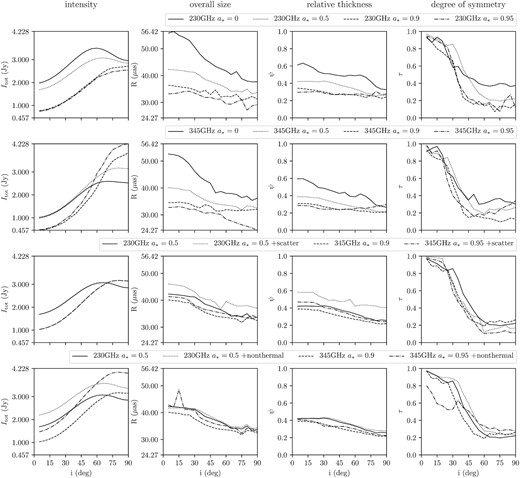
The four crescent parameters extracted from black images of inclination between 0° and 90°. Top row: spin a* =0, 0.5, 0.9, 0.95. (plotted with solid, dotted, dashed, and dash–dotted lines) at 230 GHz. Second row: same with the top row but for 345 GHz. Third row: a* =0.5, 230 GHz with/without scattering, 345 GHz with/without scattering. Bottom row: the same as the third row but for with/without non-thermal electron radiation.
