


ABSTRACT
Theories of planet formation give contradicting results of how frequent close-in giant planets of intermediate mass stars (IMSs; |$1.3\le M_{\star }\le 3.2\, \mathrm{M}_{\odot }$|) are. Some theories predict a high rate of IMSs with close-in gas giants, while others predict a very low rate. Thus, determining the frequency of close-in giant planets of IMSs is an important test for theories of planet formation. We use the CoRoT survey to determine the absolute frequency of IMSs that harbour at least one close-in giant planet and compare it to that of solar-like stars. The CoRoT transit survey is ideal for this purpose, because of its completeness for gas-giant planets with orbital periods of less than 10 d and its large sample of main-sequence IMSs. We present a high precision radial velocity follow-up programme and conclude on 17 promising transit candidates of IMSs, observed with CoRoT. We report the detection of CoRoT–34b, a brown dwarf close to the hydrogen burning limit, orbiting a 1.1 Gyr A-type main-sequence star. We also confirm two inflated giant planets, CoRoT–35b, part of a possible planetary system around a metal-poor star, and CoRoT–36b on a misaligned orbit. We find that |$0.12 \pm 0.10\, {{\ \rm per\ cent}}$| of IMSs between |$1.3\le M_{\star }\le 1.6\, \mathrm{M}_{\odot }$| observed by CoRoT do harbour at least one close-in giant planet. This is significantly lower than the frequency (|$0.70 \pm 0.16\, {{\ \rm per\ cent}}$|) for solar-mass stars, as well as the frequency of IMSs harbouring long-period planets (|$\sim 8\, {{\ \rm per\ cent}}$|).
1 INTRODUCTION
Up to now most surveys of extra-solar planets have concentrated on stars that have one solar-mass, or less (e.g. Naef et al. 2005; Cumming et al. 2008; Dong & Zhu 2013; Wittenmyer et al. 2020b) Thus, our knowledge of planets orbiting stars more massive than the Sun is currently quite limited. This is very unfortunate, because planets orbiting intermediate-mass stars give us important clues to how planets form and evolve. As intermediate-mass stars (IMSs) we denote main-sequence stars with |$M_{\star }=1.3{-}3.2\, \mathrm{M}_{\odot }$|.
Planets orbiting such stars on close orbits (with a ≲ 0.1 au) are heated up enormously making them ideal laboratories to study the inflation of planetary radii and the evaporation of planetary atmospheres (Shporer et al. 2011; Mazeh et al. 2012; von Essen et al. 2015). For example, KELT-9b, which orbits a |$M = \rm 2.5\, M_{\odot }$| star, has a day-side temperature of 4600 K, similar to a K-star (Gaudi et al. 2017). Many of them also have high obliquity’s (Winn et al. 2010). Giant planets (GP) of IMSs also give us important clues of how planets form. The lifetime of the discs of IMSs is on average about half as long but more massive than that of solar-like stars (Mamajek 2009). By studying planets of IMSs we can, thus, constrain the time-scale of planet formation.
1.1 Radial-velocity surveys of intermediate-mass stars
Using radial-velocity (RV) for this purpose is not easy. Many IMSs rotate fast with |$v\, \sin (i_\star) \gt 100\,$| km s−1 (Royer, Zorec & Gómez 2007; Pribulla et al. 2014) and many are located within the instability strip of the Hertzsprung–Russell diagram. Furthermore, the number of spectral-lines is much smaller than that of later-type stars. This limits the sensitivity for detecting IMSs planets (Galland et al. 2006a, b; Desort et al. 2009a, b; Guenther et al. 2009; Borgniet et al. 2014). The most recent result was published by Borgniet et al. (2019) who derived a frequency of |$3.7^{-1}_{+3}\, {{\ \rm per\ cent}}$| for A & F stars with masses of less than |$\rm 1.5\, M_{\odot }$| to harbour GPs closer than 2–3 au. This frequency is consistent with that of FGK-stars.
Another approach is to search for planets of giant stars that had |$1.3\le M_{\star }\le 3.2\, \mathrm{M}_{\odot }$| when they were on the main sequence (e.g. Lovis & Mayor 2007). However, the disadvantage is that giant stars may not have short period planets. Johnson et al. (2010a, b) conclude that the frequency of GPs (|$M_{\rm Planet} \ge 0.5\, M_{\rm Jup}$|) of giant and sub-giant stars at distances |$a\lt 2.5\, \rm \mathrm{au}$| increases proportional to the mass of the host star. In similar studies, Reffert et al. (2015) and Wolthoff et al. (2022) find a peak of the GP frequency at about 1.7 M⊙ which then decreases for higher mass stars again. Wittenmyer et al. (2020a) derived a GP frequency of |$7.8^{+9.1}_{-3.3}{{\ \rm per\ cent}}$| for a sample of long-period (<5 yr) planets orbiting evolved IMSs. This frequency is not significantly higher than that for solar-like stars. The surveys of giants stars, thus, indicate that the frequency of GPs of IMSs is equal, or higher than that of FGK-stars.
However, the cases of the K-giants Aldebaran (Hatzes et al. 2015; Reichert et al. 2019) and γ Draconis (Hatzes et al. 2018) and others similar (e.g. Delgado Mena et al. 2018) are worrying. Those show long-period RV variations and for a long time and it was believed that these are the signatures of planets, because they passed all the classical tests. However, after decades of observations it was discovered that the RV signal had changed, which rules out the planet hypothesis. Thus, it is possible that surveys of giant stars overestimate the planet frequency.
All RV surveys of giant stars show a lack of close-in (<0.1 au) planets. There are some hypothesis that explain that lack of close-in planets of giant stars: The first hypothesis assumes that IMSs originally had many more planets than FGK-stars, but most of them migrated inwards, for example by planet–planet scattering, or disc migration. Most of these planets ended up in orbits close to the host stars and were then engulfed when they became giants. That means we see in giant stars only those planets that were not engulfed, and these are only GPs at large distances. In the framework of this model, Hasegawa & Pudritz (2013) estimates that 5–11 per cent of main-sequence IMSs should have a close-in GP. This is one order of magnitude higher than for solar-mass stars (Naef et al. 2005; Cumming et al. 2008; Wittenmyer et al. 2020b).
The second hypothesis is that the lack of close-in planets is an effect of planet evolution. In this hypothesis, it is assumed that the migration processes are less effective for IMSs than for FGK stars. The migration time-scale for IMSs is then too long for the planets to migrate inwards. In the framework of this model, it is not expected to observe a large population of close-in GPs of IMSs. Currie (2009) predicts the frequency of close-in planets of main-sequence IMSs should be smaller than 1.5 per cent.
A possible third hypothesis would be that close-in planets evaporate due to the intense radiation of the IMSs. Nevertheless, massive Giant planets orbiting A-stars closer than 0.1 au have been detected (e.g. Cameron et al. 2010; Gaudi et al. 2017). Their existence rule out that atmospheric evaporation plays a mayor role for the lack of close-in planets orbiting such IMSs.
1.2 Transit surveys of intermediate-mass stars
As outlined in the previous section, the frequency of IMSs with close-in GPs tells us a lot about planet formation, evolution, and migration, but classical RV surveys are less than ideal for determining this number and close-in planets are not detected in surveys of giant stars.
Transit surveys have the advantage that they are not biased against rapidly rotating stars. Furthermore, they are excellent for detecting short-period planets. The first detection of a transiting GP orbiting a bright A-type star was WASP33 b (Cameron et al. 2010). Since this star is a Delta Scuti pulsator, the mass of this planet could only be measured by analysing a large amount of spectra (Lehmann et al. 2015). For transit surveys, the geometric probability to observe a transit of a planet orbiting an A5 main-sequence star with |$\rm 1.7\, R_{\odot }$| (Gray 2005) in a 6 d orbit (a = 0.08 au) is about 10 per cent. It is thus not surprising that many GP orbiting IMSs were detected in ground-based transit surveys. Examples are WASP-189b (0.05 au; Anderson et al. 2018), KELT-9b (0.03 au; Gaudi et al. 2017), KELT-21b (0.05 au; Johnson et al. 2018), or MASCARA-4b (0.05 AU; Dorval et al. 2019). Short-period brown dwarf companions can also be detected in this way. The discovery of the first transiting close-in brown dwarfs orbiting IMSs, HATS 70b (0.04 au; Zhou et al. 2019a) and TOI-503 b (0.06 au; Šubjak et al. 2020) gave us important insights how sub-stellar objects can form. As outlined by Šubjak et al. (2020), detecting such objects is particularly interesting, because it is generally thought that high-mass brown dwarfs (|$M \gt 40\, M_{\rm Jup}$|) must form in situ via core fragmentation, whereas low-mass brown dwarfs could also form in discs, just like planets.
Space-based transit surveys are perhaps the best way to determine the statistics of close-in GPs, because of their high sensitivity and the long monitoring time. The case of Kepler-13Ab shows that space-based data allow to detect planetary ephemeris from photometric variability induced by the companion (Shporer et al. 2011). The discovery of Kepler-448 b (Bourrier et al. 2015) shows that it is even possible to detect planets of IMSs with an orbital distance of more than 0.15 au.
Using planets detected by TESS (Ricker et al. 2015) and confirmed by ground-based transit surveys, like HATNet (Hungarian-made Automated Telescope Network), Zhou et al. (2019b) derived a frequency of close-in GPs of |$0.71\pm 0.31{{\ \rm per\ cent}}$| for G-stars, |$0.43\pm 0.15{{\ \rm per\ cent}}$| for F-stars, and |$0.26\pm 0.11{{\ \rm per\ cent}}$| for A-stars. This study also indicates that the frequency for IMSs is not significantly higher than that of solar-like stars as found for planets in wider orbits with radial velocity methods.
From the discovery of a peculiar features in the periodogrammes of A-stars in the Kepler data, Balona (2014) concluded that about 8 per cent of the A-type stars could have massive planets, or brown dwarf companions with orbital periods of about six days or less. However, a subsequent study by Sabotta et al. (2019) showed that these features are not caused by GPs and that the true frequency must be smaller than 0.75 per cent.
1.3 A survey for giant planets and brown dwarfs orbiting IMSs with CoRoT
CoRoT was the first space survey dedicated to the photometric search for exoplanets (Baglin et al. 2006). The detection of CoRoT–7b (Léger et al. 2009) with a transit depth of 0.03 per cent showed that space-based transit surveys are much more efficient for detecting shallow transits than ground-based surveys. According to Deleuil et al. (2018), the completeness of the CoRoT survey is about 90 per cent for GPs with orbital periods of less than 10 d. However, GPs orbiting A-stars show shallower transits than those orbiting FGK-stars, due to the larger size of the star. After several years in space, the noise limit of CoRoT in 2 h, was still about 0.1 per cent for a 15-mag star (Moutou et al. 2013). By phase-folding the light curve to the transit period the noise limit will further decrease, such that transits of GPs around IMSs can be detected with at least 5|$\, \sigma$| even for the faintest stars in the CoRoT sample which is about R = 16 mag. The completeness for GPs of A-stars, thus, is similar to that of FGK-stars.
CoRoT has observed 101 083 main-sequence stars (Deleuil et al. 2018) of which about 30 per cent are IMSs. Amongst the 36 sub-stellar companions, already published in the literature, only four are orbiting IMSs. If the frequency of GPs of IMSs were the same as that for solar-like FGK stars, we expect to find in the order of 10 GPs in this sample.
Thus, we have initiated a survey to search for close-in companions of IMSs based on the results obtained from the CoRoT–space observatory. The low RV accuracy for IMSs is not an obstacle, if we are just interested in the statistics of planets. An upper limit in the planetary regime combined with an analysis that shows that the object is not a false-positive (FP) is sufficient. Most of the known planets have been confirmed by excluding FPs, For most of them we do not have a mass determination via the RV method. An important aspect of the CoRoT mission was that all stars were searched for transits with the same method. The methods, as well as a complete list of detections and candidates are given in Deleuil & Fridlund (2018).
The preliminary results of our survey for giant planets of IMSs has been given in Guenther et al. (2016; hereafter G16). In that article, we pointed out that the stars CoRoT 110756834 (LRa02 E1 1475), CoRoT 659460079 (LRc09 E2 3322), and CoRoT 652345526 (LRc07 E2 0307) most likely harbour planets or brown dwarf companions.
In this article, we conclude our survey by presenting a detailed radial velocity analysis of our candidates, as listed in G16, including the detailed transit analysis and RV confirmation of those three objects. Furthermore, we discuss the candidate CoRoT 659668516 (LRc08 E2 4203) which was mentioned in G16 and close the cases for the remaining candidates CoRoT 110660135 (LRa02 E2 4150), CoRoT 310204242 (LRc03 E2 2657), CoRoT 102850921 (IRa01 E2 2721), CoRoT 102605773 (LRa01 E2 0963), and CoRoT 659721996 (LRc10 E2 3265).
In line with the main CoRoT survey, we will use the nomenclature for confirmed planets and brown dwarfs: CoRoT–34 (LRa02 E1 1475), CoRoT–35 (LRc09 E2 3322), and CoRoT–36 (LRc07 E2 0307), respectively for these three stars. From our results, and given the known number of IMSs that CoRoT has observed, we can now calculate the frequency of close-in GPs for IMSs and compare it with the frequency of close-in GPs for lower mass stars.
This article is structured as follows. In Section 2, we give an overview on the stellar sample, observed with the CoRoT satellite. In Section 3, we explain the selection of our candidates, being followed up in more detail. The methods used for these follow-up observations are detailed in Section 4. We introduce the sub-stellar objects discovered in our survey in Section 5 and summarize the outcome of the survey in Section 6. In Section 7, we combine the observations from the CoRoT follow-up team with our survey to draw a conclusion on the frequency of close-in GP of IMSs and discuss our results in Section 8.
2 THE STELLAR SAMPLE OF THE COROT SURVEY
In order to derive the frequency of planets for stars with different masses, we have to know how many stars of which mass the sample contains. CoRoT observed fields in two different directions in the sky. One set of fields is located close to |$\rm RA= [18^h 50^m]$|. The fields are called ‘Galactic center fields’. Stars in these fields that were observed for up to 152 d are labelled LRc (Long-Run-Center), followed by E1/E2 for the CCD used and a running number. The other fields are close to |$\rm RA= [6^h 50^m]$|. These fields are called ‘Galactic anticentre fields’ and long observing runs are labelled LRa. In preparation for the CoRoT mission, the spectral type, luminosity class, apparent brightness, and contamination factor of all stars in the fields of the CoRoT sample were determined by Deleuil et al. (2009) using multicolour photometry. The CoRoT mission was primarily designed to detect transiting planets with spectral types |$\rm \mathit{\mathit{F}}$|, |$\rm \mathit{G}$|, and |$\rm \mathit{K}$|. When selecting the targets, higher preference was given to stars that were more likely to be main-sequence F, G, K-stars but other types of stars were not excluded.
A refined photometric classification, based on the same data was published by Damiani et al. (2016). Furthermore, several spectroscopic surveys have been carried out that included a large number of these stars. Those offer an independent evaluation of the photometric classification of the sample by directly comparing the resulting spectral types.
Sarro et al. (2013) carried out a spectroscopic survey that focused on a sub-sample that has been found to be photometrically variable stars with CoroT. A large survey, focusing on solar-mass stars was published by Gazzano et al. (2010). The most comprehensive survey has been carried out by Sebastian et al. (2012) and Guenther et al. (2012) who used the multi-object spectrograph AAOmega at the AAT to determine the spectral types and luminosity classes of a representative sample of 11 466 stars in the CoRoT anticentre direction. This study shows that 32.8 per cent of all main-sequence stars in the CoRoT anticentre fields are IMSs. The comparison of the photometric and spectroscopic results by Damiani et al. (2016) showed that the median deviation between the temperatures derived photometrically and spectroscopically are only 5 per cent for late-type and 10 per cent for early-type stars, respectively. The accuracy of the luminosity classes IV and V is also within the |$\rm 1.4 \sigma$| confidence level.1 Another result from this comparison is, a systematic difference of the effective temperatures with of the adopted interstellar extinction. The photometrically derived temperatures are systematically lower for G-M type stars in the anticentre fields. Damiani et al. (2016) report the average spectroscopic distances in the centre fields to be 1.6 kpc for main-sequence stars. This is in good agreement to the distances derived by Gazzano et al. (2013). Therefore, the systematics due to extinction, found in the anticentre fields are negligible for main-sequence stars in the centre fields. Thus, the determinations are reliable and can be used to determine how many main-sequence A, F, G, K, and M-stars the sample contains.
In the next step, we estimated the stellar masses distribution of this sample by converting the spectral types to average mass ranges. We can do this by assuming main-sequence stars of solar metallicity, which is in good agreement with the findings of Gazzano et al. (2013) for the CoRoT fields. Using the conversion factors given in Gray (2005)2 we derive following upper mass limits: B7–3.2 |$\rm M_\odot$|, B9.5–2.6 |$\rm M_\odot$|, A4–2.1 |$\rm M_\odot$|, F0–1.6 |$\rm M_\odot$|, F4–1.43 |$\rm M_\odot$|, F8–1.26 |$\rm M_\odot$|, G3–1.09 |$\rm M_\odot$|, and K0–0.92 |$\rm M_\odot$|. The resulting mass-distribution for stars with luminosity classes IV and V in both viewing directions of CoRoT is shown in Fig. 1. These upper mass limits translate to a constant bin size of 0.17 |$\rm M_\odot$| for stars below 1.6 |$\rm M_\odot$| and a larger bin size of 0.5 |$\rm M_\odot$| for more massive stars.

3 IDENTIFYING THE CANDIDATES
The survey strategy is explained in detail in Guenther et al. (2016). We give a short summary on the target selection and the method, used to derive the radial velocity of the candidates. Based on both, photometric and, if available, spectroscopic classification of all CoRoT targets, we selected stars with spectral types earlier than F3 and luminosity classes IV and V. Using this criterion, we identified 25 243 CoRoT stars for which the light curves have been searched for signals of transiting planets. For this analysis, we used the EXOTRANS algorithm developed by Grziwa, Pätzold & Carone (2012). We also included all candidates identified by the CoRoT detection teams.
As planet candidates we selected all objects were the transit depth is smaller than 1.5 per cent. Since EXOTRANS is optimized to find periodic signals, after identifying the planet-candidates, we analysed their light curves in detail to derive all relevant parameters of the candidates. We removed first phase-folded the light curves and removed trends and stellar variability from each epoch using a polynomial fit. This allows to measure the transit depth, but also to investigate the light curve visually. As detailed in Ammler-von Eiff et al. (2015) all candidates were observed using the Tautenburg low-resolution (R ∼ 1000) Nasmyth spectrograph. Similarly to Sebastian et al. (2012), the spectral classification was done by comparing the spectra to catalogue reference spectra (Valdes et al. 2004) using an automatic least-square minimization pipeline. The accuracy of this method is about one to two sub-classes for IMSs (Ammler-von Eiff et al. 2015). For a first estimate of the radii of the transiting objects, we estimated the stellar radii from conversion factors given in Gray (2005).3 These radii are sufficient to remove many binary companions. However, because M-stars have roughly the same size as gas-giants, such false-positives can only be removed by RV measurements.
Since the photometric mask of CoRoT has a size of about |$\rm 30\,\mathrm{ arcsec}\times 16\,\mathrm{ arcsec}$|, it is important to confirm that the object with the transit is the bright star, and not a faint eclipsing binary within the photometric mask. Removing such false-positives (FPs) is an important step for all planet search programs. To remove these we used archival data of the CoRoT fields from the MegaPrime/MegaCam wide-field imager (Boulade et al. 2003) at CFHT, Hawaii. That data have a resolution of 0.19 arcsec pix−1 and thus allowed us to exclude bright contamination stars with a resolution of ≤1 arcsec to the candidate host-star. The 17 candidates found in this survey are listed in Table 1. The coordinates and apparent magnitudes of all candidates can be found in Table C1. Two of the candidates (CoRoT 632279463 and CoRoT 631423419) have been been ruled out as planet candidates from detailed light-curve analyses, showing a shallow secondary eclipse which only allows a binary solution for the system. Both were, thus, not followed-up with high-resolution spectroscopy.
Summary of the 17 candidates. WIN ID is the Window ID of the CoRoT data set, which has been used as reference in G16. The third to fifth columns show the spectral type and stellar mass obtained from low resolution spectroscopy, as well as the photometric detection period, respectively. The number of radial velocity measurements obtained in this study is given for each instrument. The last column shows the final status of the candidate (Special abbreviations: FD: False detection, V: stellar variability). ⋆Mass estimate from spectral type.
| CoRoT ID | Win ID | Spt | M⋆ | Period (d) | SANDIFORD | CAFE | TWIN | UVES | FIES | HIRES | HARPS | Status |
|---|---|---|---|---|---|---|---|---|---|---|---|---|
| 102806520 | IRa01_E1_4591 | A5V | 1.9⋆ | 4.29 | 6 | EB | ||||||
| 102850921 | IRa01_E2_2721 | A6V | 2.0⋆ | 0.61 | 4 | 8 | 10 | V | ||||
| 102584409 | LRa01_E2_0203 | F1V | 1.3⋆ | 1.86 | 16 | 8 | 5 | BEB | ||||
| 102605773 | LRa01_E2_0963 | F0V | 1.7⋆ | 4.65 | 3 | 16 | 4 | FD | ||||
| 102627709 | LRa01_E2_1578 | F6V | 1.3⋆ | 16.06 | 4 | EB | ||||||
| 110853363 | LRa02_E1_0725 | A5IV | 2.1⋆ | 9.09 | 5 | EB | ||||||
| 110756834 | LRa02_E1_1475 | A7V | 1.66 | 2.12 | 15 | 5 | 17 | BD | ||||
| 110858446 | LRa02_E2_1023 | F3V | 1.4⋆ | 0.78 | 4 | BEB | ||||||
| 110660135 | LRa02_E2_4150 | B4V | 2.26 | 8.17 | 14 | 7 | 10 | 2 | EB | |||
| 310204242 | LRc03_E2_2657 | A7III | 6.49 | 10.3 | 6 | 4 | 2 | BEB | ||||
| 659719532 | LRc07_E2_0108 | A9IV | 1.8⋆ | 14.45 | 7 | 13 | EB | |||||
| 652345526 | LRc07_E2_0307 | F3V | 1.32 | 5.62 | 3 | 9 | 11 | 28 | 6 | Planet | ||
| 659668516 | LRc08_E2_4203 | F3V | 2.27 | 3.29 | 6 | 4 | 2 | Candidate | ||||
| 659460079 | LRc09_E2_3322 | F3V | 1.01 | 3.23 | 8 | Planet | ||||||
| 659721996 | LRc10_E2_3265 | F6V | 2.1⋆ | 4.83 | 6 | BEB | ||||||
| 632279463 | LRc07 E2 0146 | F0V | 1.2⋆ | 0.49 | EBa | |||||||
| 631423419 | LRc07 E2 0187 | F8IV | 1.2⋆ | 3.88 | EBa |
Not followed-up with high resolution spectroscopy.
4 OBSERVATIONS AND METHODS
Given the relative faintness of our targets (|$\rm \mathit{R}=11\hbox{--}15.3\, mag$|), intermediate and high-resolution spectrographs mounted on telescopes with apertures of 2 m and larger were needed. Thus, we used a variety of instruments for the RV follow-up observations:
SANDIFORD spectrograph mounted on the Cassegrain focus of the 2.1-m Otto-Struve telescope at McDonald observatory (McCarthy et al. 1993). The grating was adjusted to achieve a wavelength coverage from 400 to 440 nm at a resolution of |$\rm \lambda /\Delta \lambda = \mathit{R}\approx 60\, 000$|. We took ThAr-frames for wavelength calibration directly before and after each spectrum to minimize radial velocity variations, introduced due to flexing of the instrument during pointings.
TWIN spectrograph at 3.5-m telescope at Calar Alto observatory, Spain. The TWIN spectrograph is a long-slit spectrograph designed for simultaneous observation in a red and blue arm.4 We observed using the T01 and T10 gratings, resulting in an intermediate resolution of |$\rm \mathit{R}\approx 7000$|. Wavelength calibration was done, using Helium–Argon exposures before and after the science spectra. Despite the relative high signal to noise, achieved for our candidates, the instrumental stability does not allow to achieve a stability of less then 10 km s|$\rm ^{-1}$|.
Calar Alto Fiber-fed Échelle spectrograph (CAFE) at the 2.2-m telescope at Calar Alto observatory, Spain (Aceituno et al. 2013). It is a fibre-fed spectrograph, which is mechanically stabilized but only passively temperature stabilized. It provides a wavelength coverage from 400 to 950 nm at a resolution of |$R\approx 60\, 000$|.
FIES spectrograph mounted on the 2.6-m Nordic Optical Telescope (NOT) at Roque de los Muchachos Observatory, La Palma, Spain (Telting et al. 2014). We used the |$\rm 1{_{.}^{\prime\prime}} 3$| high-resolution fibre, which gives a resolving power of |$R\approx 67\, 000$| and covers the wavelength range of 360–740 nm.
UVES mounted on the ESO VLT UT-2 (KUEYEN) of the ESO Paranal observatory Dekker et al. (2000). We used the standard 390 + 580 setting, which covers the wavelength region from 327 to 682 nm. Unfortunately, orders that are only partly covered by the detector, cannot be used for precise radial velocity measurements. Thus, the blue channel effectively covers only the spectral range from 329 to 452 nm without gaps and the two detectors for the red channel, cover the range from 478 to 574 nm, and from 582 to 676 nm, respectively. We used a slit-width of 0.8 arcsec, which provides a resolution of about |$R\approx 61\, 000$|.
HARPS at the ESO 3.6-m telescope at La Silla (Pepe et al. 2002; Mayor et al. 2003). The spectra cover the region from 378 to 691 nm in 72 spectral orders. Depending on the brightness of the candidate, we have obtained spectra either with the standard high accuracy mode (HAM) with a resolving power |$R\approx 115\, 000$| or the high efficiency mode (EGGS) which allows a 1.75 times higher throughput compared to the HAM mode due to a larger projected aperture of the fibre (1.4 arcsec). Depending on the actual seeing this mode offers on average a reduced resolving power of |$R\approx 80\, 000$|.
HIRES at the 10.0 Keck telescope (Vogt et al. 1994). The spectra reach a resolving power of |$R\approx 67\, 000$|.
In the following, we will briefly describe the data reduction methods used for all spectra. For HARPS, we used the HARPS pipeline to reduce and extract the spectra (bias subtraction, flat-field, scattered light subtraction, and wavelength calibration). The sky-fibre was used to remove stray-light from the moon if necessary. All other spectra were bias-subtracted, flat-fielded, the scattered light removed, and extracted using standard IRAF routines (Tody 1993). The wavelength calibration was done using calibration lamp spectra (mostly ThAr spectra for high-resolution spectrographs), obtained close to the target spectrum.
Since most of these stars are relatively faint, the signal-to-ratio (SNR) obtained was between 20 and 80. Thus, we developed a special analysis program to determine the radial velocities. In this program a synthetic or an observed high SNR spectrum is used as a template, which is fitted to the observed spectrum using the least-square method to all Echelle orders without merging them. Because the observed stellar flux in each Echelle order is larger in the centre of the blaze function, we used a weighted fit to avoid too noisy parts of the spectrum. We, thus, modelled the template using the blaze function of the Echelle spectrograph. Tests show that including the blaze function into the template improves the precision significantly. This improvement is particularly important for spectra with a low SNR (Sebastian 2017). The output is simply the relative velocity to the used template spectrum, thus, we applied the barycentric as well as the telluric-line correction for all spectra that include telluric features.
Synthetic templates were derived from line tables for different stellar parameters (Lehmann et al. 2011) to match the best parameters of the stars. However, if a sufficient number of spectra were available to reach a combined SNR larger than 50, we constructed the templates for the stars themselves by combining all these spectra taking the relative RV of the spectra to a synthetic template into account. This combination is realized by first matching all spectra by linear interpolation to the wavelength scale of the synthetic template spectrum and, second, applying a simple median function. This interpolation is applied on the level of single orders of 2D spectra which allows to combine spectral orders without additional interpolation. For determining the RV, we always used all orders, except those that contain strong telluric absorption lines. If available, telluric lines were used to monitor instrumental drifts. To measure the semi-amplitude K, as well as the orbital phase, we used a least-square optimisation to fit a Keplerian orbit to the measurements, taking the measurement errors as well as instrumental offsets into account. The photometric period was kept as a fixed parameter. We determined the error of the fit by deriving the variance of the best-fitting solutions by randomly excluding data from the sample. To test the accuracy of this method, we obtained SANDIFORD spectra of the two transiting F-type binary stars LRc07 E2 0482 (F7V, UNSW-TR-3; Hidas et al. 2005) and LRc02 E1 0132 (F3V, CoRoT 105906206; da Silva et al. 2014). Both are IMS within the same brightness-range of the candidates in our survey. LRc02 E1 0132, is a fast rotating IMS with vrotsin i⋆ ≈ 20 km s−1. We obtained six RV measurements of the primary star, well distributed over the binary orbit, and confirmed the orbit with a residual error of 60 m s−1, which is in agreement with the expected photon noise of about 200 m s−1 per measurement and including an instrumental stability of 100 m s−1.
Table 1 shows an overview of the measurements obtained per instrument. RV measurements obtained for all candidates and instruments are available as supplemental data.5
We obtained atmospheric parameters using the high-resolution spectra. For our candidates with early spectral types: CoRoT–34, CoRoT 310204242, and CoRoT 110660135 we derived the effective temperature Teff, surface gravity log (g)sp, and metallicity [Fe/H] using grids of synthetic spectra, based on ATLAS12 model atmospheres (Kurucz 1996). The most important elements were considered using a hybrid non-local thermal equilibrium (NLTE) approach with the DETAIL/SURFACE package (Giddings 1981). Our model spectra, as well as the fitting method are described in detail in Irrgang et al. (2014) and Heuser (2018). For all other candidates, the synthetic spectra were calculated in LTE using the ATLAS12 and SYNTHE codes (Kurucz 1993). To consider all sensitive features in the observed spectra, we performed global χ2 fits. In the cases where combined spectra were available from several instruments, we fitted them simultaneously using the same model grid taking different resolution and radial velocity into account. Regions that were not well reproduced were removed from the fit. This includes the cores of hydrogen lines, lines that are not included in our model spectra, as well as lines with uncertain atomic data. It is challenging to determine the surface gravity for F-type stars, because it is correlated with both the Teff and the abundance of calcium and magnesium. We assumed systemic uncertainties of 0.2 dex for log (g)sp, of 0.1 dex for [Fe/H], and 2 per cent in Teff, which were added in quadrature to the much smaller statistical uncertainties. The atmospheric parameters from spectroscopy are listed in Table 2. Second, we derived stellar age, mass, and radius by fitting the observed parameters to mesa evolutionary tracks (Choi et al. 2016) in the (Teff, |$\log \, g$|, [Fe/H]) plane as described by Irrgang et al. (2016). For CoRoT–34, 35, and 36, we used the stellar mass and radius as input for the light-curve fit, which we used to constrain log (g)lc from the light curve directly (For details, see description of the light curve fit below). We derived the final stellar age, mass, and radius as listed in Table 2 by repeating the mesa fit using log (g)lc as prior. The best-fitting evolutionary tracks are shown in Fig. 2.
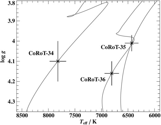
Kiel diagram showing the positions of CoRoT–34, 35, and 36. The best-fitting MIST evolutionary track (Choi et al. 2016) is shown for each star.
Parameters of the detected planets and brown dwarf companion and their host-stars. CoRoT WIN ID is the Window ID of the CoRoT data set, which has been used as reference in G16. ⋆The reported mass of CoRoT–36b is an upper limit.
| Stellar parameters | CoRoT–34 | CoRoT–35 | CoRoT–36 |
|---|---|---|---|
| RA (J2015.5) | 06 51 29.01 | 19 17 15.43 | 18 31 00.24 |
| Dec. (J2015.5) | -03 49 03.46 | -02 46 28.82 | + 07 11 00.05 |
| CoRoT ID | 110756834 | 659460079 | 652345526 |
| CoRoT Win ID | LRa02 E1 1475 | LRc09 E2 3322 | LRc07 E2 0307 |
| Gaia EDR3 id | 3102398059230983296 | 4213081309275729792 | 4477340334766250496 |
| 2MASS id | J06512900−0349034 | J19171544−0246288 | J18310024+0711001 |
| G (mag) | |$\rm 14.10\pm 0.02$| | |$\rm 15.248\pm 0.001$| | |$\rm 12.941\pm 0.03$| |
| |$\rm \mathit{K}_{S}$| (mag) | |$\rm 12.68\pm 0.04$| | |$\rm 12.94\pm 0.03$| | |$\rm 11.59\pm 0.02$| |
| aDistance (pc) | |$\rm 1540^{+210}_{-190}$| | |$\rm 1140^{+50}_{-40}$| | |$\rm 954\pm 18$| |
| Spectral type | A7 V | F6 V | F3 V |
| b|$\rm \mathit{ T}_{eff}$| (K) | |$\rm 7820\pm 160$| | |$\rm 6390\pm 130$| | |$\rm 6730\pm 140$| |
| |$^\mathit{ b} \rm log(\mathit{ g})_{sp}$| | |$\rm 3.88\pm 0.20$| | |$\rm 4.02\pm 0.2$| | |$\rm 3.92\pm 0.2$| |
| |$^\mathit{ c} \rm log(\mathit{ g})_{lc}$| | |$\rm 4.10\pm 0.10$| | |$\rm 4.01\pm 0.05$| | |$\rm 4.16\pm 0.06$| |
| |$^\mathit{ b} \rm \mathit{v}_{rot}\sin i_\star$| (km s|$\rm ^{-1}$|) | |$\rm 141.7\pm 2.7$| | 8.8 ± 0.3 | |$\rm 25.6\pm 0.3$| |
| [Fe/H]b | |$\rm -0.2\pm 0.2$| | |$\rm -0.5\pm 0.1$| | |$\rm -0.1\pm 0.1$| |
| |$\rm Age (Gyr)$| | |$\rm 1.09^{+0.19}_{-0.21}$| | |$\rm 6.1^{+1.3}_{-1.3}$| | |$\rm 2.1^{+0.6}_{-0.5}$| |
| M⋆ (M⊙) | |$\rm 1.66^{+0.08}_{-0.15}$| | |$\rm 1.01^{+0.07}_{-0.06}$| | |$\rm 1.32^{+0.09}_{-0.09}$| |
| |$\rm \mathit{R}_{\star } (R_{\odot })$| | |$\rm 1.85^{+0.29}_{-0.25}$| | |$\rm 1.65^{+0.10}_{-0.11}$| | |$\rm 1.52^{+0.20}_{-0.10}$| |
| Fitted parameters | CoRoT–34b | CoRoT–35b | CoRoT–36b |
| Period (d) | |$\rm 2.11853\pm 0.00006$| | |$\rm 3.22748\pm 0.00008$| | |$\rm 5.616531 \pm 0.000023$| |
| Phot. epoch (|$\rm BJD_{TDB}$|) | |$\rm 2454787.7411\pm 0.0016$| | |$\rm 2456074.2415 \pm 0.0018$| | |$\rm 2455662.52236\pm 0.00034$| |
| |$\rm \mathit{b}_{\rm rr}$| | |$\rm 0.0609\pm 0.0022$| | |$\rm 0.1047\pm 0.0017$| | |$\rm 0.0953\pm 0.0013$| |
| |$\rm \mathit{b}_{\rm rsuma}$| | |$\rm 0.244\pm 0.025$| | |$\rm 0.197\pm 0.010$| | |$\rm 0.121\pm 0.008$| |
| K (km s|$\rm ^{-1}$|) | |$\rm 7.68\pm 0.85$| | |$\rm 0.15\pm 0.05$| | |$\rm 0.065\pm 0.045$| |
| e (fixed) | 0 | 0 | 0 |
| Companion parameters | CoRoT–34b | CoRoT–35b | CoRoT–36b |
| |$\rm \mathit{a}_\mathrm{b}$| (au) | |$\rm 0.03874 \pm 0.00081$| | |$\rm 0.04290\pm 0.00092$| | |$\rm 0.066\pm 0.007$| |
| |$\rm i_\mathrm{b}$| (deg) | |$\rm 77.8_{-1.6}^{+1.4}$| | |$\rm 84.1\pm 0.1$| | |$\rm 85.83\pm 0.26$| |
| |$\rm \mathit{b}_\mathrm{tra;b}$| | |$\rm 0.92\pm 0.02$| | |$\rm 0.58_{-0.07}^{+0.06}$| | |$\rm 0.573_{-0.025}^{+0.023}$| |
| Transit depth (mmag) | |$\rm 3.34_{-0.17}^{+0.21}$| | |$\rm 11.47\pm 0.31$| | |$\rm 9.214_{-0.10}^{+0.099}$| |
| Ttot; b (h) | |$\rm 2.02_{-0.11}^{+0.12}$| | |$\rm 4.19\pm 0.08$| | |$\rm 4.98\pm 0.07$| |
| Quadr. limb u1 | |$\rm 0.32\pm 0.08$| | |$\rm 0.25\pm 0.15$| | |$\rm 0.27_{-0.07}^{+0.06}$| |
| Quadr. limb u2 | |$\rm 0.17\pm 0.08$| | |$\rm 0.28\pm 0.17$| | |$\rm 0.24_{-0.09}^{+0.12}$| |
| |$\rm \mathit{M}_\mathrm{b}$| (|$\mathrm{\mathit{M}_{\rm Jup}}$|) | |$\rm 71.4_{-8.6}^{+8.9}$| | |$\rm 1.10_{-0.37}^{+0.37}$| | |$^\star \rm 0.68_{-0.43}^{+0.47}$| |
| |$\rm \mathit{R}_\mathrm{b}$| (RJup) | |$\rm 1.09_{-0.16}^{+0.17}$| | |$\rm 1.68\pm 0.11$| | |$\rm 1.41\pm 0.14$| |
| |$\rm \rho _b (g\, cm ^{-3})$| | |$\rm 60\pm 21$| | |$\rm 0.29\pm 0.11$| | |$\rm 0.25\pm 0.17$| |
| |$\rm \mathit{T}_\mathrm{eq;b}$| (K) | |$\rm 2425_{-128}^{+137}$| | |$\rm 1747\pm 62$| | |$\rm 1567\pm 35$| |
Displayed distances were determined by spectrophotometry for CoRoT–34, and from Gaia EDR3 parallaxes for CoRoT–35, and 36.
Parameters derived from high-resolution spectroscopy.
|$\rm log(\mathit{g})_{lc}$| derived from light-curve fitting.
Reliable parallaxes from the early third Gaia release (EDR3, Gaia Collaboration et al. 2021; Lindegren et al. 2021a; El-Badry, Rix & Heintz 2021) allow us to derive precise distances. For CoRoT–34, however, the EDR3 quality parameters6 indicate an inconsistent parallax measurement. Thus, we derived Gaia EDR3 distances for CoRoT–35 and CoRoT–36 only, by applying the parallax zero-point offset following Lindegren et al. (2021b). For CoRoT–34, we derived the spectrophotometric distance from the spectral energy distribution (SED) along with the interstellar reddening and using log (g)lc as prior (see Appendix A). We fitted the SED also for CoRoT–35 and 36 and found that the effective temperature derived from the SED consistently agrees with the spectroscopic effective temperature. The SED fitting also allows us to derive the angular diameters which are displayed in Table A1.
The CoRoT data were obtained from the IAS CoRoT Public Archive.7 We used the Version 4 legacy data release, which had been extensively reprocessed over the original CoRoT releases (Chaintreuil et al. 2016). We used the BAR fluxes, which had been corrected from aliasing, offsets, backgrounds, the jitter of the satellite, differences in the flux due to the change of the mask, the change of the temperature set point, and the loss of long-term efficiency. Furthermore, spurious points were replaced by interpolation. Of note is that the time-stamps in the legacy release are given in Barycentric Dynamical Time (BJD_TDB), instead of the heliocentric UTC time of the previous Versions 1–3, which were used as the basis of all previous CoRoT planet discoveries. The difference between the two time-scales is about one minute – for details on this topic, please refer to Eastman, Siverd & Gaudi (2010).
The CoRoT light curves were then corrected from stellar variability, as well as residual instrumental effects. For this fit we masked the transit times, which were known from the detection ephemeris and periods. To allow for slight changes in these parameters, we included each 30 min out of transit time before and after the predicted transit time into the mask. We modelled the light curve using a polynomial fit by applying the Chebyshev function, implemented in the (numpy.polynomial)8 package. The polynomial order was determined visually to only model variability on longer time-scales that the expected transit duration. In this way, we were able to account for intensity variations due to pulsations that would affect the transit shape. To finally model the transit light curve, we used the software package ALLESFITTER (Günther & Daylan 2019) which uses the ellc (Maxted 2016) eclipse model to fit the transit light curve. The main fitting parameters are the orbital period P, the transit epoch, the dimensionless planet–star radius ratio brr = Rb/R⋆, as well as brsuma = (R⋆ + Rb)/a, which both parameterise the scaled semimajor axis a/R⋆ = (1 + brr)/brsuma. R⋆ is the stellar radius, Rb the planetary radius, and a the semimajor axis. Further orbit parameters are |$\rm cos(i_b)$|, with the inclination |$\rm i_b$| which can be used to derive the impact factor |$\rm \mathit{b}_{tra;b}$|, as well as the parameters |$\rm \mathit{f}_c = \sqrt{e} cos(\omega)$| and |$\rm \mathit{f}_s = \sqrt{e} sin(\omega)$|, with the eccentricity |$\rm e$| and the longitude of periastron |$\rm \omega$|. The limb darkening is parametrized using the quadratic parameters u1 and u2 which were sampled using the parameters q1 and q2 as defined in Kipping (2013). We sampled the posterior probability distribution (PPD) of the model parameters using nested sampling (Speagle 2019). In order to optimise the run-time we used wide uniform priors based on transit parameters, derived from a preliminary solution obtained from a least-squares fit. We used a stellar density prior from stellar mass and radius estimates, derived from spectroscopy and took the dilution within the CoRoT mask into account. We then used the function massradius from the software package pycheops (Maxted et al. 2021) which applies a Monte Carlo approach to derive physical system parameters from the sampled parameter |$\rm period$|, |$\rm \mathit{a}/\mathit{R}_\star$|, |$\rm \mathit{b}_{\rm rr}$|, |$\rm cos(\mathit{i}_b)$|, the radial velocity semi-amplitude K, as well as the stellar mass and radius estimates. For CoRoT–34, 35, and 36, we derive the stellar density directly from Keplers third law and the before mentioned light-curve parameters (Seager & Mallén-Ornelas 2003), which we used to derive the surface gravity log (g)lc of the host star. We used this to optimize the mass and radius of the host stars, but also of the planets and brown dwarf. As a comparison, we listed in Table 2 the surface gravity derived from spectroscopy (log (g)sp), as well as that from the light-curve fit (log (g)lc).
5 SUB-STELLAR COMPANIONS DISCOVERED
As we will show in this section, CoRoT–34 (CoRoT 110756834) is a mid A-type star with a companion that is just at the border between a very low-mass star and a brown dwarf, and CoRoT–35 (CoRoT 659460079), as well as CoRoT–36 (CoRoT 652345526) are mid F-type stars, with each harbour a giant planet.
5.1 CoRoT–34
5.1.1 Exclusion of background sources for CoRoT–34
This star was discovered as a transit candidate in the original CoRoT survey with a short period of about 2.12 d. Guenther et al. (2013) obtained adaptive optic imaging and spectroscopy in the K band, using CRIRES at the VLT at the Paranal Observatory. They excluded any background eclipsing binary (BEB) earlier than K3V within 0.8 arcsec and ruled out any physical companion earlier than F6V. Furthermore, they excluded all stars in and close to the CoRoT mask being eclipsing binaries, using seeing-limited imaging obtained with CFH12K prime focus camera of the 3.6-m Canada France Hawaii Telescope (CFHT; located at Mauna Kea, Hawaii, USA). All these observations confirmed that the transit originates from the star itself and not from a background star within the PSF.
5.1.2 Analysis of the CoRoT light curve of CoRoT–34
The star was observed with CoRoT between 2008 November |$\rm 16$| and 2009 March |$\rm 11$|. Thanks to the star’s brightness, three colour light curves have been obtained. Sarro et al. (2013) used CoRoT light curves combined with stellar parameters derived from Giraffe spectra to automatically classify different pulsation pattern. They classified CoRoT–34 as a pulsating star with a period of 1.4 d. By inspecting the light curve, we find, that the pulsation period is actually half this period (0.71 d) with a variable amplitude of up to 1 per cent. After detrending the light curve for these pulsations, we used the colour information to determine the transit depth in all three bands. Despite increased noise in the blue and green CoRoT light curves, we cannot see any significant decrease in transit depth, and, thus, can exclude any late-type BEB of K or M-type. This is also supported by the non detection of any infrared excess by fitting the SED of CoRoT–34 (see Fig. A1). The phase folded light curve is shown in Fig. 3 and all derived transit parameters are listed in Table 2.
Upper panel: Phase folded, light curve of CoRoT–34. The red line is the best-fitting model, using a dilution factor of Fcont/Fsource = 0.014. The lower panel shows the residuals from the transit fit.
5.1.3 High-resolution spectroscopy of CoRoT–34
We obtained 5 spectra with HIRES, 17 spectra with HARPS (using the HAM mode, under ESO programme 184.C-0639) and 15 spectra with UVES (under ESO programme 092.C-0222) over a total time-span of 3.1 yr. We used the combined HARPS and UVES spectra to derive atmospheric parameters from our global spectral fit. The resulting parameters for |$\rm \mathit{T}_{eff}$|, |$\rm log(\mathit{g})_{sp}$|, [Fe/H], and |$\rm \mathit{v}_{rot}\sin \mathit{i}_\star$| are listed in Table 2 which are consistent with the values derived by Sarro et al. (2013). Unfortunately, these would put CoRoT–34 close to the termination of the main-sequence evolution, that is to the end of core hydrogen burning, making it difficult to derive the stellar mass and radius because of the changing shape of the evolutionary tracks. From the distribution of best-fitting evolutionary tracks within the spectroscopic uncertainties, we derive a mass of |$1.76^{+0.28}_{-0.15}$| M⊙, which we used as a prior to fit the light curve. |$\rm log(\mathit{g})_{lc}$|, derived from the light curve, allowed us to constrain the stellar mass and radius of CoRoT–34 (see Fig. 2), which are listed in Table 2.
The star is fast rotating with |$v\, \sin (i_{\star }) = 141.7\pm 2.7$| km s|$\rm ^{-1}$|, which complicates the mass determination of the companion. We used our least-square fitting method, and got a good fit with a mean accuracy of 100 m s|$\rm ^{-1}$|. Nevertheless, the radial velocity varies by several km s|$\rm ^{-1}$| even for spectra taken in the same night. One possible explanation is the impact of stellar oscillations leading to distortions of the line profile. In order to measure this effect, we modelled the least-squares deconvolution (LSD) line profiles (Donati et al. 1997) for each spectrum using a line list, with line weights optimised for an IMS with |$\mathit{T}_{\rm eff} = 8000\, K$| and |$\rm log(\mathit{g}) = 4.0$| (Lehmann et al. 2011) based on data from the Vienna Atomic Line Database (VALD; Kupka et al. 2000). The LSD profile clearly shows the distortions of the line-profile caused by the pulsations. Since the magnitude of the observed distortions is only a fraction of the broadened line profile, a simple Gaussian least-squares fit is used to obtain the mean velocity. In a second step, we calculated the integral of the profile to account for the asymmetry of the profile as a measure of the line distortions. The variance of both measurements is, thus, used as uncertainty. The UVES spectra showed an instrumental offset between the blue and red CCD. We decided to measure both spectra individually, correct for the constant offset and average the RV measurements. The RV results are listed in Table B3.
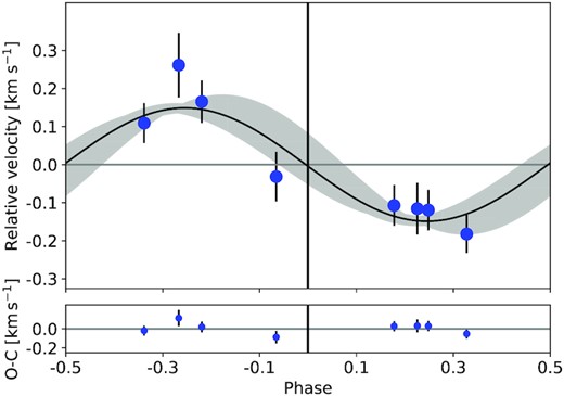
The radial velocity curve has been constructed from all high resolution spectra to determine the mass of the companion. The phase folded RV measurements for all instruments are shown in Fig. 4. We found an orbital solution that is in perfect agreement with the photometric period and ephemeris. The residuals of the orbital fit follow a Gaussian distribution which we have verified using a Kolmogorov–Smirnov test by comparing it to a Gaussian-distributed sample. The standard deviation of the residuals is |$\rm 2.6\, km\, s\rm ^{-1}$|, which is smaller than the average uncertainty of our RV measurements. Thus, we can conclude that the orbital solution is (i) stable for data obtained with different instruments, (ii) stable over several years, and (iii) independent from the variable photometric amplitude of the stellar pulsations. Using the known orbit inclination, we derived the mass of the companion and found it to be a high-mass brown dwarf close to the hydrogen burning limit with an extreme mass ratio q = |$\rm \mathit{M}_{BD}/\mathit{M}_{\star }$| = |$\rm 0.0412\pm 0.0048$|. All parameters derived for this object are given in Table 2.
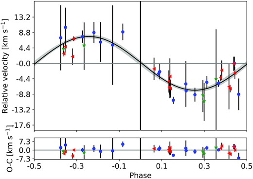
Upper panel: Phase folded, radial-velocity curve of CoRoT–34. Blue points: HARPS measurements; green triangles: HIRES measurements; red triangles: UVES measurements. The photometric epoch of the transit is at phase = 0. The black lines shows the best-fitting orbital solution, with the grey area depicting the uncertainty of the fit. The lower panel shows the residuals from the orbital fit.
5.2 CoRoT–35
5.2.1 Excluding background sources for CoRoT–35
The transit was discovered during LRc09, the last Galactic center fields observation run of CoRoT, with a transit depth of |$1{{\ \rm per\ cent}}$|.
Using the CFH12K prime focus camera of the CFHT we obtained on and off transit images on 2021 August |$\rm 27\,$| and |$\rm 28\,$|. These images show that CoRoT–35 is |$\rm 0.0097\pm 0.0026$| mag fainter during the transit. No other nearby star showed a significant change in brightness. We, thus, conclude that CoRoT–35 is the star with the transit. The images show no stars in the direct vicinity and the dilution factor is |$\rm 0.5\pm 0.2{{\ \rm per\ cent}}$|, which is small, compared to other targets in this survey (which is usually |$\rm \gt 1{{\ \rm per\ cent}}$|).
5.2.2 Analysis of the CoRoT light curve of CoRoT–35
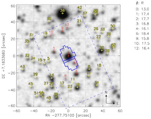
CoRoT–35 was observed in monochromatic mode for 84 d in 2012 from April |$\rm 12\,$| to July |$\rm 7\,$|, first with the low cadence mode (8.5 min), and after the star has been found to be transiting with the high cadence mode (32 s). Fig. 5 shows an DSS image taken with the CoRoT-mask superimposed. Twenty six transits have been observed and we found that the transit mid-times vary by up to one hour during the CoRoT observations. This strongly hints for another massive, but possibly sub-stellar object orbiting CoRoT–35. To model the out-of-transit variations using a polynomial fit, we increased the transit mask to 1.5 h before and after the predicted transit times to account for the mid-time variations. After the out-of-transit variations were corrected, we modelled the mid-time variations using ALLESFITTER and took these into account to model the transit parameters from the light curve and to determine the size and other parameters of the planet. The mid-time variations are listed in Table D1, the phase folded light curve is shown in Fig. 6. Despite the fit does agree well with the data, we note a small hump during the transit about 0.7 h after the transit mid-time. Such humps generally could hint for stellar activity such as spot crossing events. Since our transit model does not include spot crossing events, our fit might underestimate the planet-to-star radius ratio (e.g. Oshagh et al. 2014). Given the magnitude of |$\rm \mathit{R}=15.28$|, the light curve of CoRoT–35 has larger uncertainties, compared to the other companions found in this survey, thus spot crossing events are not resolved in individual transits. We repeated our transit fit using a different binning of 36 min, to increase the photometric precision of the data, and derived similar transit parameters compared to our initial fit, but find no sign of a hump. We conclude that it is more likely an artefact from white and residual red-noise of the light curve. All results of the transit fit are listed in Table 2.
DSS image of CoRoT–35 with the photometric mask overlaid. North is up, and east is on the right.

Phase folded, light curve of CoRoT–35. The red line is the best-fitting model. The lower panel shows the residuals from the transit fit. Blue points represent the data binned to 12 min.
5.2.3 High-resolution spectroscopy of CoRoT–35
We took 8 spectra of CoRoT–35 with the HARPS spectrograph using the EGGS mode (under ESO programme 188.C-0779). The stellar parameters from our global spectral fit are listed in Table 2. It shows CoRoT–35 to be a late F-type star that is slowly rotating. We found that the star is relatively metal-poor. This is in line with its comparatively low mass of |$\rm \mathit{M}_\star = 1.01\pm 0.13\,M_\odot$| and old age of |$\rm \approx 6\, Gyr$| as derived from MIST evolutionary tracks. Using the optimized |$\rm log(\mathit{g})_{lc}$| from the light curve fit, we again derived the stellar mass and radius from evolutionary tracks (see Fig. 2). In this case, the |$\rm log(\mathit{g})_{sp}$| from spectral fitting matches well the light-curve fit, but given the improved accuracy of |$\rm log(\mathit{g})_{lc}$| we were able to better constrain the stellar radius which is listed in Table 2.
Since the rotational velocity is with |$\rm \mathit{v}_\mathrm{rot}\sin \mathit{i}_\star \lt 10\, km\, s\rm ^{-1}$| relatively small, we determined the RVs using the classical cross-correlation method with a numerical mask that corresponds to a G2 star (Baranne et al. 1996; Pepe et al. 2002). The RV measurements were obtained by fitting a Gaussian function to the average cross-correlation function (CCF), after discarding the ten bluest and the two reddest orders of the spectra that were of too low SNR. The results are given in Table B4. One of the eight HARPS spectra, taken on 2013 September |$\rm 9\,$|, deviates slightly (|$\rm \lt 1.5\, \sigma$|) from the orbital solution. This particular night suffered from strong wind (|$\rm \gt 15\, m\, s\rm ^{-1}$|) and variable seeing conditions (1.1–1.7 arcsec), reducing the SNR to about 50 per cent, and increasing the relative error compared to the other data. Fig. 7 shows the best orbital fit to the HARPS measurements.
Phase folded radial-velocity measurements of CoRoT–35b from HARPS. The photometric epoch of the transit is at phase = 0. The black curve represents the best-fitting orbit model, with the grey shaded region depicting the uncertainty of the fit. The lower panel shows the residuals from the orbital fit.
5.3 CoRoT–36
5.3.1 Excluding a background binary within the photometric mask of CoRoT–36
To exclude that CoRoT–36 is an FP, we used seeing limited imaging as well as adaptive imaging. The rate and nature of FPs in the CoRoT exoplanets search, and the way how to detect and remove FPs is described in Almenara et al. (2009).
5.3.1.1 Seeing limited imaging of CoRoT–36
As part of the ground-based photometric follow-up for CoRoT candidates (described in Deeg et al. 2009), we obtained time-series imaging of CoRoT–36 during two predicted transits. Both were acquired in R band, one with the WISE-1-m telescope on 2011 September |$\rm 9\,$| 2011 and the other one with the IAC-80-cm telescope on 2014 July |$\rm 25\,$| (Fig. 9). The light curves and transit mid-times from both transits have been published in (Deeg et al. 2020). A comparison of Fig. 8 with Fig. 9 shows that the stars labelled with F20 and F22 are just outside the mask but star F24 is inside. Both data sets show that the target varied by an amount that would correspond to the depth of the transit, whereas the variations of the other stars are at least one order of magnitude less than what would be expected for an FP. The data obtained with the WISE telescope were obtained 73 d after the end of the CoRoT-observations and contained only an egress, whereas the IAC-80 observations were obtained over 3 yr later, and contained a nearly complete transit. The IAC-80 timing given in Deeg et al. (2020) was, therefore, converted to the BJD_TDB time-scale of the CoRoT data, and was used to derive an orbital period with a precision (see Table 2) that is significantly improved over one based only on the CoRoT data.
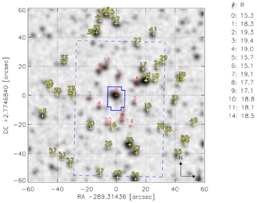
DSS image of CoRoT–36 with the photometric mask of CoRoT overlayed. North is up, and east is on the right.
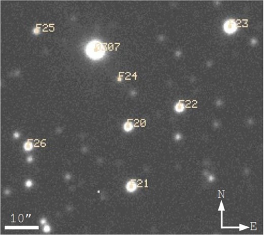
Image taken of CoRoT–36 (labelled as 0307) with the 0.8-m telescope of the IAC. North is up, and east is on the right. The size of the image is about |$\rm 60\times 60 \,arcsec$|, and the orientation is the same as in Fig. 8. The stars labelled with F20 and F22 are just outside the mask but star F24 is inside.
5.3.1.2 Adaptive optics imaging of CoRoT–36
In critical cases AO-imaging is essential for confirming transiting planets, otherwise the probability for an FP is unacceptably high. We consider CoRoT–36b a critical case, because it is very difficult to confirm the planet by RV measurements due to the stellar rotation.
Observations were carried using PISCES (Guerra et al. 2011) together with the First Light Adaptive Optics (FLAO; Esposito et al. 2010) system mounted on the Large Binocular Telescope (LBT). PISCES was the first adaptive optical imager of the LBT, but it is now decommissioned. It was equipped with a 1kx1k Hawaii-1 (HgCdTe) detector which provided an images scale of 0.019 arcsec pixel−1. For optimal sky-subtraction, the images were obtained by jittering. The final images were then obtained by co-adding the overlapping region. Since the size of the image shown in Fig. 10 is only |$\rm 6\times 8\,arcsec$|, the star labelled F24 in Fig. 9 is far outside the field of view. A disadvantage of adaptive optics imaging is that the observations are taken at infrared wavelengths, whereas CoRoT observes within the optical. From the depth of the transit, and the brightness of the star, we concluded that FPs have to be brighter than V = |$\rm 18.13\pm 0.07$| mag. Because of the extinction, faint background stars are much brighter at infrared wavelength than in the optical. Faint stars in the foreground have typically also red colours, due to being late-type stars, unless they are white dwarfs or subdwarfs. We imaged the object in the J and K band. This does not only allow us to determine the colours of any potential background object but it also helps to distinguish artifacts from real objects.
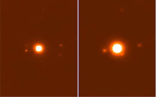
Images taken with the AO-system PISCES at the LBT in the K (left) and in the J band (right). The size of the image is only about 6 × 8 arcsec, north is up and east is left. Two previously unknown stars at distances of |$\rm 1{_{.}^{\prime\prime}} 96\pm 0{_{.}^{\prime\prime}} 04$| and |$\rm 3{_{.}^{\prime\prime}} 46\pm 0{_{.}^{\prime\prime}} 04$| are visible. The orientation is as in Fig. 9.
We detected two previously undetected stars. Star No. 1 is |$\rm 1{_{.}^{\prime\prime}} 94\pm 0{_{.}^{\prime\prime}} 02$| W, |$\rm 0{_{.}^{\prime\prime}} 30\pm 0{_{.}^{\prime\prime}} 03$| S, and has |$\rm J=15.7\pm 0.1$|, |$\rm \mathit{K}=16.2\pm 0.1$|, and star No. 2 is |$\rm 3{_{.}^{\prime\prime}} 42\pm 0{_{.}^{\prime\prime}} 02$| E, |$\rm 0{_{.}^{\prime\prime}} 53\pm 0{_{.}^{\prime\prime}} 02$| N, and has J = 17.1 ± 0.1, K = 16.8 ± 0.1. Both stars are not visible in the images taken with the WISE and IAC-80-cm telescopes, but are identified in the Gaia DR3 catalogue as Gaia DR3 4477340339082969856 (G = 18.12), and Gaia DR3 4477340339063864064 (G = 19.96) for star No. 1 and 2, respectively. The Gaia parallaxes excluded both stars to be physical companions. Star No. 2 is clearly too faint in the optical to be an FP. Despite star No. 1 is in the optical at the limiting magnitude to cause an FP, we can rule out this scenario as by-product of our spectroscopic transit observations (see Section 5.3.3).
5.3.2 Analysis of the CoRoT light curve of CoRoT–36
The star was continuously observed with the CoRoT satellite over a period of 81.2 d from 2011 April |$\rm 8\,$| to June |$\rm 28\,$|. In total 218 441 intensity measurements were obtained in three colors with a time-sampling of 32 s. Fig. 8 shows an DSS image with the CoRoT mask superimposed. The observations were taken with a roll angle of 23.967o and an image scale of 2.32 arcsec pixel−1. The images of the stars are elongated, because of the bi-prism which provides the three colour photometry. In total 15 transits can be seen in the raw-data. We divided the CoRoT light curve by a polynomial model to remove any long-term variability of the star. Fig. 11 shows the phase-folded light curve, as well as, the best-fitting transit model with the orbital eccentricity set to zero. The derived transit parameters are given in Table 2.
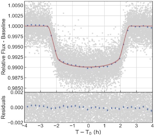
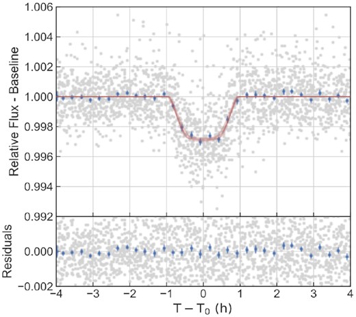
Phase folded, white light curve of CoRoT–36. The red line is the best-fitting model. The lower panel show the residuals from the transit fit. Blue points represent the data binned to 12 min.
5.3.3 Spectroscopic observations of CoRoT–36
Radial velocity measurements of CoRoT–36 were taken for two purposes: first to constrain the mass of the planet, and second to independently confirm the planet using time resolved transit spectroscopy.
We obtained 9 measurements with 30-min exposure time, reaching an SNR of about 80 with the TWIN spectrograph in 2014 June and 3 measurements with the SANDIFORD spectrograph. We observed CoRoT–36 with 30-min exposures, resulting in an average SNR of about 80. The instrumental stability does not allowed us to use these spectra to exclude a stellar companion for the orbital period. Therefore, we used these data to determine the spectral type listed in Table 1. The accuracy of the SANDIFORD spectra is, however, sufficient to rule out a massive binary companion. To finally narrow down the planet mass, we used two different instruments. Using the fibre-fed Echelle spectrograph FIES, we obtained 11 spectra of CoRoT–36 in four observing runs between 2012 June and 2013 June. The data were reduced as described in Section. 3. Additionally, six spectra of CoRoT–36 were obtained with HARPS in EGGS mode between 2012 June|$\rm 15\,$| and July |$\rm 10\,$| under ESO program 188.C-0779. Due to the lack of instrumental stability, we excluded the RV measurements obtained with the TWIN and SANDIFORD spectrographs, but used our measurements obtained with HARPS and FIES. Because of the line broadening due to stellar rotation, it is very difficult to determine the radial velocity variation caused by a Jupiter-mass companion. Nevertheless, we fitted all the different runs, by using instrumental offsets as free parameters, which allowed us to narrow down the semi-amplitude of the orbit. The best-fitting parameters are listed in Table 2, the orbital fit is shown in Fig. 12. Given the large uncertainties in the data, this measurement is rather an upper limit and confirms CoRoT–36b to be a Jupiter-mass planet. All RV measurements, covering the orbital phase are listed in the Appendix, Table B1.
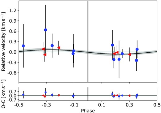
Phase folded radial-velocity measurements of CoRoT–36b obtained out of transit with HARPS (red triangles) and FIES (blue points). The photometric epoch of the transit is at phase = 0. The black curve represents the best-fitting orbit model, with the grey shaded region depicting the uncertainty of the fit. The lower panel shows the residuals from the orbital fit.
While the rotation is a problem for precise RV observations, it opens up the possibility to confirm the planet by Doppler imaging (e.g. Bouchy et al. 2008). Comparing out-of-transit spectra with spectroscopic time series taken during the transit allows us to confirm the presence of a transiting object, to determine its relative size, and its orbital inclination relative to the spin-axis of the star.
We obtained two independent data sets of the transit. The first with 17 FIES spectra on 2013 July |$\rm 25\,$|. We used as templates the average spectrum of the target, by excluding the telluric lines.
Another data set of 11 spectra was obtained with UVES in service mode (on 2013 August |$\rm 6\,$|). Each in-transit spectrum was exposed for 970 s, the out-of-transit spectrum was exposed for 1450 s. The in-transit observations were obtained for |$\rm 2^h55^m$|, and the out-of-transit spectrum was taken |$\rm 2^h9^m$| after the end of in-transit observations in the same night. By taking the out-of-transit spectrum in the same night, we minimized the risk for any variations of the point-spread function, and we ensured that the out-of transit observations were certainly taken after the transit had ended. The achieved SNR at 600 nm was on average 240 per resolution element.
The RV measurements of both data sets are listed in the Appendix, Table B2. The measurements obtained with FIES are relative velocities in respect to the template used. We applied an RV offset of 22.79 |$\rm km\, s\rm ^{-1}$| to best match both data sets during the overlapping phase, This is possible since both data sets have been observed in- and out-of-transit. We find that both data sets agree very well and show an almost constant drift between the measurements taken out and in transit, due to the Rossiter–McLaughlin (RM) anomaly, a change in the stellar line profile due to the ‘shadow’ of the planet. We used the RV model of ellc (Maxted 2016) and the Markov chain Monte Carlo (MCMC) code EMCEE (Foreman-Mackey et al. 2013) to sample the model parameters, using the sampled parameters from the light-curve fit as priors. The resulting RV data and best-fitting RV model is shown in Fig. 13. We concluded that the planet has to be in a nearly polar orbit with a projected angle between the orbital axis of the planet and the spin axis of the star |$\rm \lambda _b = 275.8 \pm 11.3$|.
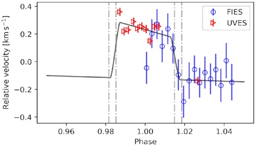
RV measurements obtained for CoRoT–36 during the transit with UVES (red points) and FIES (blue triangles). The best-fitting RM model is shown as black line. The dashed lines indicate the position of the transit.
We used high-resolution spectra obtained with UVES and HARPS to determine the atmospheric parameters |$\rm \mathit{T}_{\rm eff}$|, |$\rm log(\mathit{g})_{sp}$|, as well as the rotational velocity |$v\, \sin (i_{\star })$|. The stellar parameters, radius and mass, derived from evolutionary models confirm it to be an early F-type star with a mass of |$\rm 1.49^{+0.20}_{-0.18}\, M_\odot$|. We used this mass as prior for the light curve fit to optimize the surface gravity |$\rm log(\mathit{g})_{lc}$|, which we used to optimize the stellar mass and radius using evolutionary models. All derived stellar parameters are listed in Table 2 and are, within the errors, consistent with the values reported in Boufleur et al. (2018).
We used the fact that both stars No. 1 and 2 (see Section 5.3.1) are well resolved in the UVES acquisition images, which allowed us to monitor their brightness during and out-of-transit. None of these stars show a notable drop in brightness, which rules out both to cause a potential FP.
Thus, all the evidence speaks for a close-in giant planet in polar orbit. All parameters derived for this object are given in Table 2.
6 DISCARDED CANDIDATES
In the previous sections, we have presented three cases for transiting objects, discovered in this survey. Two are giant planets, and one is an object that is at the border between a brown dwarf and a low-mass M-star. In this section, we will discuss CoRoT 659668516, and show that the transit does not originate from the star itself. We, furthermore, summarize the outcome for the remaining candidates, showing that these are not planets orbiting IMSs.
Seven of our candidates have been identified as eclipsing binaries and are listed in Table 1. CoRoT 632279463 and CoRoT 631423419 have been identified as binaries by analysing the CoRoT light curves and have not been followed up with high-resolution spectroscopy (see Section 3). The candidate CoRoT 110660135, which has been identified as binary, from intensive high-resolution spectroscopic follow-up, will be discussed in more detail in the next section. The four candidates CoRoT 102806520, CoRoT 102627709, CoRoT 110853363, and CoRoT 659719532 have been identified due to large drifts of several km s|$\rm ^{-1}$| in consecutive spectra. Due to the sparse coverage of their orbits, we did not derive their orbital solutions. Nevertheless, we list the RV measurements of all candidates in the supplementary material.
6.1 CoRoT 659668516
CoRoT 659668516 is a F3V star that has been observed by CoRoT between 2011 July |$\rm 7\,$| and 2011 September |$\rm 30\,$| in monochromatic mode. The light curve shows transits with a period of |$\rm 3.287022_{-1.3e-05}^{+1.5e-05}$| d. Two contaminating sources (Gaia DR3 4284693601105758592, G = 19.1 mag and Gaia DR3 4284693601087059328, G = 17.7 mag), hereafter S1 and S2, have been identified within 3 arcsec of the star. Since all of them are in the mask of CoRoT, we derived a dilution factor as the sum of the contributing flux, relative to the main source (G = 15.2 mag) |$\rm \mathit{F}_{blend} / \mathit{F}_{source} = 0.13$|. Fig. 14 shows the phase-folded light curve. Despite the ephemeris are well constraint, the errors are too large to allow additional photometric follow-up from the ground, additionally this target has not been observed by TESS. Six intermediate resolution spectra were taken with the TWIN spectrograph mounted at 3.5-m telescope at Calar Alto observatory which showed a possible BD solution for the companion. In order to find out what the nature of these eclipses are, we obtained four spectra with UVES and analysed two HARPS spectra, taken 2.1 yr before the UVES observations. We determined the stellar parameters with |$\rm \mathit{T}_{\rm eff}=7080\pm 200\, K$|, |$\rm log(\mathit{g})=3.37\pm 0.30$|, |$\rm [Fe/H]=0.0\pm 0.2$|, and a projected rotational velocity of |$v\, \sin (i_{\star })=64\pm 2\,$|km s|$\rm ^{-1}$|. For these parameters, we obtained its mass and radius with |$M_{\star }=2.27\pm 0.27\, \mathrm{M}_{\odot }$| and |$\rm \mathit{R}_{\star } = 5.06\pm 1.3\, R_{\odot }$|. The UVES spectra also show that the spectrum is composite with a slowly rotating component. Due to the blended spectrum, deriving accurate stellar parameters for this component is challenging. We found |$\rm \mathit{T}_{\rm eff}=6340\pm 300\, K$|, |$v\, \sin (i_{\star })=5\pm 3\,$|km s|$\rm ^{-1}$|, and obtained |$M_{\star } = 1.24\pm 0.1\, \mathrm{M}_{\odot }$| and |$\rm \mathit{R}_{\star } = 1.45\pm 0.24\, R_{\odot }$| if a surface gravity of 4.2 dex is assumed for a star close to the zero-age main-sequence. The blend is unlikely to originate from the visually resolved stars, since S1 is too faint to generate the blend and S2 has been excluded during the UVES and HARPS observations. From these stellar parameters, it is very likely that the transit does not originate from the brighter, fast rotating component since the measured transit duration of |$\rm 3.75\pm 0.07$| h is 2 to 3 times shorter than expected for any companion orbiting a star with |$\rm 5.06\, R_{\odot }$|. Since a large impact parameter is not supported by the transit shape, this scenario would require an eccentric orbit. Since our least-squares fit method cannot be used to measure the relative velocity of a composite spectrum, we measured the slowly rotating component using the cross-correlation with a numerical G2 mask and the fast rotating component by measuring the LSD profiles. The RV measurements are listed in the Appendix, Table B5. Both components do not show any relative or absolute change in RV over the 2.1 yr, which excludes a spectroscopic binary with the 3.29-d period. In sum, this transit signal originates either from an object orbiting the slow rotating IMS, or from a BEB residing within the photometric mask of CoRoT.
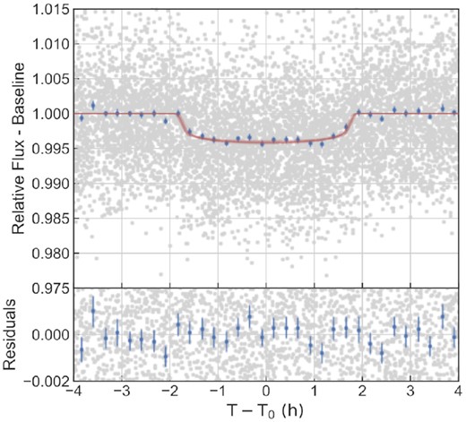
Phase folded, white light curve of CoRoT 659668516. The red line is the best-fitting model. The lower panel shows the residuals from the transit fit.
6.2 Other discarded candidates
CoRoT 310204242 has been observed in chromatic mode by CoRoT. We identified it to show a planet-like transit with an orbital period of 5.15 d. Despite being an evolved star, it drew our attention as the light curve in different colours did not show a clear depth difference and TWIN spectra showed RV variations, comparable with those expected for a BD companion. The two HARPS spectra of this star do not have sufficient SNR to measure the RV of this rapidly rotating star. We obtained and analysed four UVES spectra. The star is an A-giant with |$\rm \mathit{R}_{\star } = 3.43\pm 0.6\, R_{\odot }$|, |$\rm \mathit{T}_{\rm eff}=7670\pm 160\, K$|, |$\rm log(\mathit{g})=3.25\pm 0.21$|, and a rotational velocity of |$v\, \sin (i_{\star })=126\pm 1\,$|km s|$\rm ^{-1}$|. Despite that no close contaminant has been found, using seeing limited observations, the UVES spectra are clearly composite with a slow rotating |$v\, \sin (i_{\star })=3.6\,$| km s|$\rm ^{-1}$| component. The RV measurements do not show a large variation, but match to an orbital solution with |$\rm \mathit{K} \approx 1.5$| km s|$\rm ^{-1}$| and an orbital period of 10.3 d which is twice the period, found from the light curve. We re-analysed the CoRoT light curve using the new orbital period and found that the target has to be a bright object with about |$\rm 5\, \mathit{R}_{Jup}$| with a secondary eclipse that is about half as deep as the primary eclipse. Albeit, the blue and red CoRoT light curves do not show any change in eclipse depth, the eclipse is twice as deep in the green light curve. This colour effect can only be noted by phase folding the light curve with the right orbital period. The data fit best to a BEB, which contaminates part of the CoRoT mask and is bright enough to also contaminate the RV measurements.
CoRoT 110660135 is a B-star that shows pulsations of 1.7d with 12 mmag amplitude and transit-like signals with a period of |$\rm 8.17041\pm 0.00008\, d$|. The prospect of a possible discovery of a planet orbiting a B-star initiated our detailed RV follow-up on this target, which finally confirmed that this object is a triple system with a close binary component. We covered the orbital phase spectroscopically with spectra from SANDIFORD, CAFE, FIES, and HARPS. Using HARPS spectra, we derived the stellar parameters and found it to be a very young B-type star with |$\rm \mathit{R}_{\star } = 2.26\pm 0.8\, R_{\odot }$|, |$\rm \mathit{T}_{\rm eff}=15900\pm 400\,$| K, and a high surface gravity (|$\rm log(\mathit{g})=4.44\pm 0.11$|). The latter places the star close to the zero age main-sequence (ZAMS) in the HRD and, thus, it is probably a very young star with an age of less than 4 Myr. Due to its grazing eclipse configuration, the size of the companion is not well constrained by the best fit to the CoRoT light curve. Nevertheless, using the stellar parameters, the radius of the companion has to be |$\rm 2.6\pm 1.0\, \mathit{R}_{Jup}$|, which indicates a possible late-type stellar companion. A detailed inspection of the LSD line profiles shows, that, CoRoT 110660135 is indeed a SB2. The stellar rotation with |$v\, \sin (i_{\star })=33.1\,$| km s|$\rm ^{-1}$| makes it difficult to measure the reflex motion of the orbit. To combine the radial-velocity measurements from all observations, we had to correct for a linear trend of |$\delta v_{\mathrm{rad}}=-7.3\,$| km s|$\rm ^{-1}$| yr|$\rm ^{-1}$|, which implies the presence of another unresolved stellar companion, orbiting CoRoT 110660135 in a long-period orbit.
Other candidates have been discarded by more detailed analysis of their light curves. The transit signal of CoRoT 102850921 has been mimicked by stellar pulsations and the transit of CoRoT 102605773 could not be confirmed after the star has been re-observed with CoRoT in LRa06. Additionally to these, there are three candidates that turned out to be background eclipsing binaries (BEB). (i) CoRoT 102584409, is an SB2, but with a much longer period, as found with CoRoT. (ii) For CoRoT 659721996, we do not see any RV variation, and derive an upper limit of 3.8 km s|$\rm ^{-1}$| (|$\rm \mathit{M}_{Pl}\lt 30\, M_{\rm Jup}$|), corresponding to a low-mass BD. Nevertheless, the light curve shows a periastron brightening which has to be caused by a very luminous companion or most likely a BEB. (iii) For CoRoT 110858446, available spectra point at a blend with another star that turned out to be a BEB.
7 THE FREQUENCY OF IMSS WITH CLOSE-IN GIANT PLANETS
With the completion of the CoRoT survey we can now determine the frequency of IMSs to harbour close-in gas giant planets (GPs) and compare it to that of solar-mass stars. As close-in GPs we count transiting companions with |$\rm \mathit{a} \lesssim$| 0.1 au and |$\rm \mathit{R}_{Pl} \gt 0.8\, \mathit{R}_{Jup}$| in the planetary regime which is consistent to Deleuil et al. (2018). Thirtysix planets and BDs (34 of them transiting) in 33 planetary systems9 have been found with CoRoT after observing 163 665 stars of which 101 083 are dwarfs (luminosity class IV and V, Deleuil & Fridlund 2018). The stellar population of this sample has been studied in detail (see Section 2). Deleuil et al. (2018) derived a frequency for this sample of |$\rm 0.98\pm 0.26{{\ \rm per\ cent}}$| to host GPs with orbital periods of less than 10 d.
Four of the published systems meet our mass-criterion for IMSs (|$M_{\star }=1.3{-}3.2\, \mathrm{M}_{\odot }$|). These are the two brown dwarfs CoRoT–3b (|$M_{\star }=1.37\pm 0.09\, \mathrm{M}_{\odot }$|; Deleuil et al. 2008), and CoRoT–15b (|$M_{\star }=1.32\pm 0.12\, \mathrm{M}_{\odot }$|; Bouchy et al. 2011), as well as the GPs CoRoT–11b (|$M_{\star }=1.56\pm 0.10\, \mathrm{M}_{\odot }$|; Gandolfi et al. 2010; Tsantaki et al. 2014) and CoRoT–21b (|$M_{\star }=1.29\pm 0.09\, \mathrm{M}_{\odot }$|; Pätzold et al. 2012). The latter is within its errors just at the border of being an IMS. In this article, we presented the cases for CoRoT–34b and CoRoT–36b, and gave evidence that first is a brown dwarf, orbiting an A-star of |$\rm 1.66\, \mathrm{M}_{\odot }$| and the latter is GP orbiting an F-star of |$\rm 1.32\, \mathrm{M}_{\odot }$|. Despite that we can show CoRoT–35b being a GP orbiting an F-star, the mass of its host star (|$M_{\star } = 1.0\, \mathrm{M}_{\odot }$|) falls well below our mass-criterion for IMSs. We also discussed the remaining candidate for a sub-stellar companion of CoRoT 659668516 and found it likely to orbit an |$\rm \mathit{M} = 1.24\pm 0.1\, \mathrm{M}_{\odot }$| star residing within the photometric mask, which is at the border of being an IMS.
That means that with the CoRoT survey three GPs of IMSs with spectral type F have been found, but none with a host mass larger than 1.6|$\, \mathrm{M}_{\odot }$|. On the other hand, CoRoT detected three brown dwarfs orbiting IMS with one of them orbiting an A-type star. Given these discoveries, we can derive the frequency for IMSs to host close-in GPs and, thus, further extend the results from Deleuil & Fridlund (2018) to early F-type stars with 1.6 M⊙.
Applying our before-mentioned limits for close-in giant planets, we excluded in this statistic (i) close-in brown dwarfs (CoRoT–3b, CoRoT–15b, CoRoT–33b, and CoRoT–34b), (ii) planets with sizes from the terrestrial to Neptune regime (CoRoT–7b, CoRoT–22b, CoRoT–24b, and CoRoT–32b), (iii) planets with orbital periods longer than 10 d (CoRoT–9b, CoRoT–10b, and CoRoT–24c), and (iv) the non transiting CoRoT–7c and CoRoT–20c without direct radius measurement. The resulting sample contains 26 transiting GPs with host star masses between |$\rm 0.88\pm 0.04\, \mathrm{M}_{\odot }$| and |$\rm 1.56\pm 0.1\, \mathrm{M}_{\odot }$|, taking into account the updated host star masses for CoRoT–3 and CoRoT–11 (Tsantaki et al. 2014). This selection leads to a sample of 26 GPs detected with CoRoT.
This result enables us to directly compare the number of host stars (with at least one GP detected) to the number of stars analysed by CoRoT, in order to derive the planet frequency. To calculate how many IMSs have been analysed, we cross-matched the stellar population for main-sequence stars (see Section 2) with the total number of stars with CoRoT light curves (without duplication) obtained via EXODAT10 (Deleuil et al. 2009). Here, we denoted main-sequence stars as classified with IV and V from the Galactic anticentre fields (Guenther et al. 2012) as well as the Galactic centre fields (Damiani et al. 2016) with a magnitude limit of r′ < 15.4 (Corresponding to the faintest planetary host stars found by the CoRoT survey). As in Section 2, we select the mass interval of 0.75–3.2 M⊙ to include the lowest mass GP host star, as well as the whole sample of IMS observed with CoRoT, leading to 70 525 stars with 33 846 IMSs. We divided the sample of 26 detected GP host stars according to their mass, in the same mass interval we have used for the stellar sample in Section 2. To derive the GP frequency from the number of stars in each mass bin, we assume an average error of 0.1 M⊙ and derived the uncertainty of the GP frequency from the variance of the different resulting solutions.
Assuming arbitrary inclinations, we can correct for the geometric transit probability |$\rm \mathit{ p}=\mathit{R}_{\star }/\mathit{a}$|, because we can only detect transiting objects. We derive this correction for each of the 26 GPs individually, reaching a mean transit probability of 12.1 per cent This means that the true number of close-in GP host stars in the CoRoT sample is more than 250.
By combining the corrected GPs, as well as the stellar sample from the centre and anticentre fields, we derive a GP frequency of |$\rm 0.70 \pm 0.16\, {{\ \rm per\ cent}}$| for FGK stars (0.75–1.26 M⊙), assuming a detection efficiency of 90 per cent. This result is only slightly different when including the candidate CoRoT 659668516 into the sample (|$\rm 0.71 \pm 0.15\, {{\ \rm per\ cent}}$|). This is consistent, but slightly smaller compared to Deleuil et al. (2018) (|$\rm 0.98 \pm 0.23\, {{\ \rm per\ cent}}$|), who used a slightly brighter magnitude limit, as well as a smaller sample of stars for the comparison.
We find a GP frequency of |$\rm 0.12 \pm 0.1\, {{\ \rm per\ cent}}$| for IMSs between 1.26 and 1.6 M⊙11 (|$\rm 0.10 \pm 0.1\, {{\ \rm per\ cent}}$|, when adding CoRoT 659668516 into the sample.) The GP frequency versus stellar mass is shown in Fig. 15. For comparison we added the normalized stellar sample and like to point out that the majority of planet host stars detected with CoRoT are of solar mass, while the majority of stars, surveyed with CoRoT are early F-type stars with masses between 1.1 and 1.2 M⊙. The absence of many F-type planets in the sample, thus, leads to a steep decline of the planet frequency for stars more massive than 1.1 M⊙.
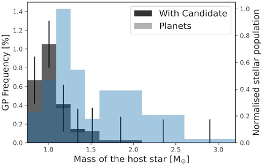
GP Frequency of the CoRoT sample for FGK and IMS stars. Grey, frequency based on confirmed planets, dark grey, including the candidate CoRoT 659668516. Light blue: the stellar sample, observed with CoRoT.
About 5900 IMS with masses |$\rm \gt 1.6\, \mathrm{M}_{\odot }$| have been observed with CoRoT. The absence of planet detections in this sample does not allow to derive a GP frequency directly. Nevertheless, we can derive an upper limit by deriving the GP frequency, in the case at least one GP host star would have been detected. We assumed an detection probability of 12 per cent for a 10 d orbit to derive the upper limit of |$\rm 0.25 \pm 0.16\, {{\ \rm per\ cent}}$| for the mass range between 1.6 and 3.2 M⊙.
8 SUMMARY AND CONCLUSIONS
The CoRoT survey is one of the few photometric surveys that allow us to determine the frequency of close-in planets of IMSs on the main-sequence. As IMSs, we denote main-sequence stars with |$M_{\star }=1.3{-}3.2\, \mathrm{M}_{\odot }$|. Roughly one third of the main-sequence stars that have been observed with CoRoT are stars in this mass range. The sensitivity of the mission is large enough to detect all objects with |$\rm \mathit{R}_{planet} \gt 0.8\, \mathit{R}_{Jup}$| orbiting at |$\rm \mathit{a} \lesssim$| 0.1 au with a completeness rate of better than 90 per cent. That means CoRoT has the sensitivity to detect basically all transiting, close-in gas-giant (GP) planets, brown dwarfs and stellar companions. In our survey, we analysed all IMSs, observed by CoRoT and studied 17 promising candidates in detail. Only three of them could be confirmed as close-in sub-stellar companions:
CoRoT–34b, is a brown dwarf with |$\rm \mathit{M}_{BD}= 71.4_{-8.6}^{+8.9}\, M_{\rm Jup}$| and, thus, just below the hydrogen burning limit which marks the border towards low-mass stars. Only ≈30 transiting BDs, that allow to directly measure their mass and radius, are known to date. Since CoRoT–34b is fully transiting, the transit parameters are well defined, which make it to an important test bench for testing models of high-mass BDs. Its mass and radius lead to a surface gravity |$\rm log(\mathit{g})_{BD} = 5.14 \pm 0.10$|, which is slightly lower than predicted from models at an stellar age of about 2.1 Gyr (e.g. Baraffe et al. 2003; Saumon & Marley 2008; Phillips et al. 2020). This can possibly be explained by the inflated radius of |$\rm 21\pm 13\, {{\ \rm per\ cent}}$| compared to the COND03 model (Baraffe et al. 2003). This apparent discrepancy would be resolved if the BD were inflated by the irradiation from its host star. Acton et al. (2021) showed in their Fig. 7, the relationship between equilibrium temperature and radius for known transiting BDs. Notably all known BDs with |$\rm \mathit{T}_{equ} \gt 2000\,$| K have radii larger than predicted by evolutionary models of BDs at the age of their host stars. These are HATSs-70b (Zhou et al. 2019a), KELT-1b (Siverd et al. 2012), and TOI-503b (Šubjak et al. 2020), which span, together with CoRoT–34b, through the whole mass-range of BDs from deuterium burning to the hydrogen burning limit. The fact that it turned out that CoRoT–34b is an inflated 2.1 Gyr old BD at the hydrogen burning limit, may allow us to study possible heating mechanisms by stellar irradiation and their dependence from the mass of the BD. Since high-mass BDs thought to be formed in situ, it might also be possible that further, non-transiting sub-stellar companions with orbital periods <100 d exist around CoRoT–34 (Batygin, Bodenheimer & Laughlin 2016). We find that CoRoT–34 pulsates with 0.71 d, which is only a bit shorter, but very close to one third of the orbital period. This strong synchronization of the stellar pulsations with the orbit of the brown dwarf might be explained by tidally excited oscillation modes caused by the close-in Brown dwarf as a result of tidal circularization (Kumar, Ao & Quataert 1995).
CoRoT–35b and CoRoT–36b are both giant planets which show anomalously large radii, only consistent with the largest known hot Jupiters. Those anomalous radii are probably best explained by heating processes related to the strong irradiation from their host stars, which lead to equilibrium temperatures larger than 1700 and 1500K, respectively (Sarkis et al. 2021). The discovery of CoRoT–35b plays a particularly interesting role, as it orbits a metal-poor star. The CoRoT centre fields are located at low Galactic latitudes, which are dominated by stars of solar metallicity in the galactic thin disc, which makes CoRoT–35 a rather exceptional object in the CoRoT sample (Gazzano et al. 2013). Only very few metal-poor stars (|$\rm [Fe/H] \lt -0.3 dex$|) have been confirmed to host hot Jupiters and up to date less than ten of them have GPs with inflated radii larger than |$\rm 1.4\, \mathit{R}_{Jup}$|.12 Examples of such objects are WTS-1b (Cappetta et al. 2012) or KELT-21b (Johnson et al. 2018). We found transit timing variations for CoRoT–35b, hinting at another massive planet in the system. Only 26 transits have been observed with CoRoT, thus, it will be difficult to model the object causing these variations (e.g. Veras & Ford 2009). In future research, this can be done by adding more data points, for instance, using ground- or space-based photometry, which will allow to measure the mass of this object. Along the same line, many published CoRoT planets have recently been re-observed by TESS, allowing to optimise the transit periods and ephemeris (Klagyivik et al. 2021). The possibility to find a planetary system together with the rarity of such inflated GPs orbiting stars with sub-solar metallicity, makes the detection of CoRoT–35b a rare benchmark object for the planet formation of such stars (e.g. Adibekyan 2019).
With time-resolved transit spectroscopy, we confirm that CoRoT–36b is orbiting in a polar orbit with a projected obliquity of |$\rm 275.8 \pm 11.3\, ^{\circ }$|. This discovery adds CoRoT–36b to the growing list of misaligned giant planets, orbiting IMSs. It has been confirmed that more massive stars tend to have commonly misaligned planets in nearly circular orbits (e.g. Winn et al. 2010). This misalignment is generally thought to be triggered by the Kozai mechanism due to an perturbing object, like an outer planet (e.g. Nagasawa, Ida & Bessho 2008; Triaud et al. 2010; Winn et al. 2010). Other mechanisms might play a role to explain the observed distribution of planet obliquities (see Albrecht, Dawson & Winn 2022, for a review).
One of our candidates, CoRoT 659668516, still might be a sub-stellar object of an ISM, but is very diluted by other sources, and thus, we cannot conclude on its nature. All other candidates were identified as false signals or binary stars, and therefore, we can extend the frequency of close-in Giant planets of IMSs, and compare it to the frequency of solar-type stars.
We determine the frequency of solar-type stars in the CoRoT sample to host at least one close-in giant planet to |$\rm 0.70 \pm 0.16\, {{\ \rm per\ cent}}$|. This result is fully consistent to the findings from other surveys for close-in planets from solar-type stars like Naef et al. (2005) (|$0.7\pm 0.5\, {{\ \rm per\ cent}}$|), Cumming et al. (2008) (|$0.64\pm 0.4\, {{\ \rm per\ cent}}$|), Mayor et al. (2011) (|$0.89 \pm 0.36\, {{\ \rm per\ cent}}$|), and Zhou et al. (2019b) (|$0.71 \pm 0.31\, {{\ \rm per\ cent}}$|).
For stars with |$M_{\star }=1.26 {-} 1.6\, M_\odot$|, we derive an average GP frequency of |$\rm 0.12 \pm 0.10\, {{\ \rm per\ cent}}$| and find a steep drop in this mass range. The upper mass limit of |$\rm 1.6\, M_\odot$| is selected to include the highest mass planet host stars, identified with CoRoT.
Due to the large number of early F-type stars, surveyed during the CoRoT mission, and its high detection efficiency this is a significant result, which cannot be explained by selection effects within the mission design. We can, thus, exclude any increase of the close-in GP-frequency in this mass range within the CoRoT survey. For stars more massive than IMSs, we derive an upper limit of 0.25 per cent.
This GP frequency for IMS is well in agreement with the upper limits derived from the Kepler space mission (<0.75 per cent, Sabotta et al. 2019) but slightly lower than the preliminary results obtained from the TESS space mission for F-type stars (0.43 ± 0.15 per cent, Zhou et al. 2019b). This difference can be explained by the wider mass-range of our survey which includes a steep decline of the GP frequency for stars more massive than |$\rm 1.4\, M_\odot$| which was used as upper border in their study. Our upper limit for the GP frequency of stars with masses between |$\rm 1.6 \,and\, 3.2\, M_\odot$| is fully consistent with the frequency for more massive IMS, found in TESS.
This is in contrast to the GP frequency at larger separations, from RV surveys of giant stars, that show an increase with stellar mass (e.g. Johnson et al. 2010a, b; Reffert et al. 2015). Assuming that this higher planet frequency for IMSs is not overestimated by stellar activity, we can conclude that the efficient migration scenario, which would lead to a higher frequency for close-in planets, that are then engulfed during stellar evolution (e.g. Hasegawa & Pudritz 2013), cannot play a large role to explain the absence of short period GPs in RV surveys. Nevertheless, it cannot fully be ruled out since such close-in GPs do exist (e.g. Zhou et al. 2019b).
SUPPORTING INFORMATION
radial_velocities.csv
Please note: Oxford University Press is not responsible for the content or functionality of any supporting materials supplied by the authors. Any queries (other than missing material) should be directed to the corresponding author for the article.
ACKNOWLEDGEMENTS
The CoRoT space mission, launched on 2006 December |$\rm 27$|, has been developed and is operated by CNES, with the contribution of Austria, Belgium, Brazil, ESA (RSSD and Science Programme), Germany, and Spain. This work was support by the Deutsche Forschungsgemeinschaft (DFG) through grants GU 464/15- 1,GU 464/16-1, GU 464/17-1, GU 464/18-1, andTs 17/2-1. EG and DS also acknowledge the generous support by the Thüringer Ministerium für Wirtschaft, Wissenschaft und Digitale Gesellschaft. CH, UH, AI, and MD acknowledge funding by the Deutsche Forschungsgemeinschaft (DFG) through grants HE1356/62-1, HE1356/71-1, andIR190/1-1. This research is also supported work funded from the European Research Council (ERC) the European Union’s Horizon 2020 research and innovation programme (grant agreement n° 803193/BEBOP). HJD acknowledges support from the Spanish Research Agency of the Ministry of Science and Innovation (AEI-MICINN) under grant PID2019-107061GB-C66, DOI: 10.13039/501100011033. JK gratefully acknowledges the support of the Swedish National Space Agency (DNR 2020-00104). This research has made use of the SIMBAD data base, operated at CDS, Strasbourg, France. We made also use of data from the European Space Agency (ESA) mission Gaia (https://www.cosmos.esa.int/gaia), processed by the Gaia Data Processing and Analysis Consortium (DPAC, https://www.cosmos.esa.int/web/gaia/dpac/consortium). The ground- based observations were obtained with the VLT at the European Southern Observatory at Paranal, Chile (291.C-5028(A), 092.C- 0222(A), and 093.C-0027(A), with the 2.2-m and 3.5-m telescope at German-Spanish Astronomical Center at Calar Alto (H12-2.2-037, H14-2.2-043), with the Nordic Optical Telescope at La Palma (NOT runs P45-109, P45-206, P46-113, P46-215, P47-105, P47-211, P48-217, P49-205; funding from the European Union Seventh Framework Programme FP7/2013-2016 under grant agreement No. 312430, OPTICON), the 2.1-m at McDonald observatory, Texas, the 80-cm telescope of the Instituto de Astrofisica de Canarias at the observatorio del Teide, the Tel-Aviv University 1-m telescope at WISE Observatory, the Alfred-Jensch telescope in Tautenburg, and the Large Binocular Telescope. The NOT is operated on the island of La Palma jointly by Denmark, Finland, Iceland, Norway, and Sweden, in the Spanish Observatorio del Roque de los Muchachos of the Instituto de Astrofisica de Canarias. The 2.2-m and 3.5-m telescopes of the Calar Alto observatory is located in the Sierra de Los Filabres (Andalucia, Southern Spain) north of Almeria. It is operated jointly by the Max-Planck-Institut for Astronomie (MPIA) in Heidelberg, Germany, and the Instituto de Astrofisica de Andalucia (CSIC) in Granada/Spain. The LBT is an international collaboration. LBT Corporation partners are: The University of Arizona on behalf of the Arizona university system; Istituto Nazionale di Astrofisica, Italy; LBT Beteiligungsgesellschaft, Germany, representing the Max-Planck Society, the Astrophysical Institute Potsdam, and Heidelberg University; The Ohio State University, and The Research Corporation, on behalf of the University of Notre Dame, University of Minnesota, and University of Virginia. This publication makes use of data products from the Two Micron All Sky Survey, which is a joint project of the University of Massachusetts and the Infrared Processing and Analysis Center/California Institute of Technology, funded by the National Aeronautics and Space Administration and the National Science Foundation. The authors thank the referee for the constructive remarks.
DATA AVAILABILITY
Most data underlying this article is available online as indicated in the specific section or reference. Data, obtained with ESO telescopes are available in the ESO Science Archive Facility, at http://archive.eso.org/cms.html. Other data underlying this article will be shared on reasonable request to the corresponding author.
Footnotes
85 per cent agreement between photometric and spectroscopic classification.
Book page 506, Table B.1.
Book page 506, Table B.1.
RV measurements are available in machine readable form as radial_velocities.csv.
The re-normalised unit weight error, RUWE (Lindegren 2018), as well as the ipd_gof_harmonic and ipd_frac_multi parameters are inspected.
The Extrasolar Planets Encyclopedia (Schneider et al. 2011) (2021 August).
For the stellar sample, we use the same binning as in Section 2 with 1.26 M⊙ being the lower border of the bin that includes the 1.3 M⊙ limit for IMSs.
NASA exoplanet archive, 2021 August.
REFERENCES
APPENDIX A: SPECTROPHOTOMETRIC TEMPERATURE, ANGULAR DIAMETER, AND INTERSTELLAR REDDENING
The spectroscopic analysis provided us with the atmospheric parameters. The spectral energy distribution (SED) provides us with an independent estimate of the effective temperature (see Table A1). Making use of the geometric flux dilution we derive the angular diameter (Θ = 2R/d) as a scaling factor from the observed flux f(λ) and the synthetic stellar surface flux F(λ): Θ2 = f(λ)/F(λ)/4. Because the CoRoT stars are located at low Galactic latitude interstellar reddening is important to be accounted for. We fit the interstellar colour excess and the RV parameter simultaneously with the angular diameter and the effective temperature, using the reddening law of Fitzpatrick et al. (2019). For CoRoT–34 the SED is well covered (see Fig. A1) allowing us to determine the RV parameter of the reddening law to be close to the standard (RV = 3.0). The synthetic flux distributions are interpolated from a grid of model SEDs calculated with the atlas12 code and matched to the observed magnitudes by χ2 minimization (see Heber, Irrgang & Schaffenroth 2018; Irrgang et al. 2020, for details). The surface gravity and metallicities of the stars are fixed. The results are summarized in Table A1. Effective temperatures agree well with the spectroscopic ones listed in Table 2.
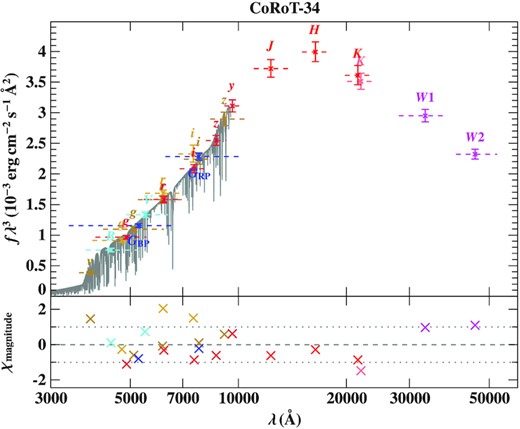
Comparison of synthetic and observed photometry for CoRoT–34. Top panel: SED with filter-averaged fluxes (times wavelength to the power of three) converted from observed magnitudes. The approximate width of the respective filters (widths at 10 per cent of maximum) are shown by dashed lines. The best-fitting model SED, smoothed to a spectral resolution of 6 Å, is shown in grey. Bottom panel: Residuals χ, i.e. the difference between synthetic and observed magnitudes divided by the corresponding uncertainties. The different photometric systems are displayed in the following colours: APASS-griz (golden, Henden et al. 2015); PAN-STARRS (red, Chambers et al. 2017); SkyMapper (dark yellow, Onken et al. 2019); APASS-Johnson (cyan, Henden et al. 2015); Gaia (blue, Riello et al. 2021); 2MASS (red, Skrutskie et al. 2006); UKIDDS (pink Lawrence et al. 2007); UNWISE (magenta, Schlafly, Meisner & Green 2019).
Resulting parameters of the fit of the spectral energy distributions.
| CoRoT–34: | |
|---|---|
| Color excess E44 − 55) | |$0.323^{+0.040}_{-0.029}$| mag |
| Extinction parameter R(55) | |$3.67^{+0.23}_{-0.21}$| |
| Angular diameter |$\log (\Theta \, \mathrm{(rad)})$| | |$-10.259^{+0.007}_{-0.016}$| |
| Effective temperature Teff | |$7820^{+320}_{-220}$| K |
| CoRoT 35: | |
| Color excess E(44 − 55) | |$0.566^{+0.022}_{-0.049}$| mag |
| Angular diameter |$\log (\Theta \, \mathrm{(rad)})$| | −10.254 ± 0.010 |
| Effective temperature Teff | |$6400^{+120}_{-260}$| K |
| CoRoT 36: | |
| Color excess E(44–55) | |$0.206^{+0.020}_{-0.097}$| mag |
| Angular diameter |$\log (\Theta \, \mathrm{(rad)})$| | |$-10.030^{+0.016}_{-0.020}$| |
| Effective temperature Teff | |$6800^{+100}_{-520}$| K |
APPENDIX B: RADIAL VELOCITY MEASUREMENTS
The following tables list the RV measurements for the confirmed Sub-stellar companions CoRoT–34b, 35b, and 36b, as well as for the candidate CoRoT 659668516. All other RV measurements are available in machine readable form as supplementary material.
Radial velocity measurements of CoRoT–36 obtained during several orbital phases out of transit. Horizontal lines mark data sets obtained with different instruments or different observing runs.
| HJDa | RV | ±σ | Instrument |
|---|---|---|---|
| -2 450 000 | (km s|$\rm ^{-1}$|) | (km s|$\rm ^{-1}$|) | |
| 6093.80675 | 10.18 | 0.20 | HARPS |
| 6096.67636 | 9.99 | 0.20 | HARPS |
| 6098.79155 | 10.15 | 0.20 | HARPS |
| 6101.67704 | 10.01 | 0.20 | HARPS |
| 6115.70754 | 9.98 | 0.20 | HARPS |
| 6118.64215 | 10.05 | 0.20 | HARPS |
| 6101.60540 | 9.68 | 0.43 | FIES |
| 6102.58413 | 9.24 | 0.30 | FIES |
| 6104.50742 | 10.12 | 0.72 | FIES |
| 6107.49199 | 9.27 | 0.54 | FIES |
| 6118.51460 | 9.28 | 0.24 | FIES |
| 6119.45816 | 9.58 | 0.26 | FIES |
| 6120.45199 | 9.68 | 0.63 | FIES |
| 6121.62526 | 9.68 | 0.34 | FIES |
| 6122.49860 | 9.53 | 0.48 | FIES |
| 6459.46791 | 9.65 | 0.27 | FIES |
| 6461.46262 | 9.65 | 0.13 | FIES |
| 6115.69276 | 19.95 | 0.21 | SANDIFORD |
| 6116.85210 | 19.02 | 0.25 | SANDIFORD |
| 6117.80003 | 18.09 | 0.26 | SANDIFORD |
The Heliocentric Julian date is calculated directly from the UTC.
Radial velocity measurements of CoRoT–36 obtained during and close to the transit.
| HJDa | RV | ±σ | Instrument |
|---|---|---|---|
| −2 450 000 | (km s|$\rm ^{-1}$|) | (km s|$\rm ^{-1}$|) | |
| 6499.3910 | −0.044 | 0.116 | FIESb |
| 6499.4059 | 0.202 | 0.104 | FIES |
| 6499.4207 | 0.272 | 0.108 | FIES |
| 6499.4356 | 0.112 | 0.116 | FIES |
| 6499.4517 | 0.238 | 0.112 | FIES |
| 6499.4665 | 0.097 | 0.108 | FIES |
| 6499.4814 | −0.095 | 0.112 | FIES |
| 6499.4963 | −0.289 | 0.116 | FIES |
| 6499.5123 | −0.138 | 0.132 | FIES |
| 6499.5272 | −0.056 | 0.100 | FIES |
| 6499.5420 | −0.151 | 0.108 | FIES |
| 6499.5569 | −0.078 | 0.116 | FIES |
| 6499.5729 | −0.124 | 0.112 | FIES |
| 6499.5878 | −0.058 | 0.116 | FIES |
| 6499.6026 | −0.171 | 0.120 | FIES |
| 6499.6176 | 0.008 | 0.128 | FIES |
| 6499.6336 | −0.148 | 0.132 | FIES |
| 6510.5485 | 23.150 | 0.030 | UVESc |
| 6510.5604 | 23.010 | 0.030 | UVES |
| 6510.5722 | 23.020 | 0.030 | UVES |
| 6510.5873 | 23.080 | 0.030 | UVES |
| 6510.5992 | 23.030 | 0.030 | UVES |
| 6510.6110 | 23.045 | 0.030 | UVES |
| 6510.6231 | 23.025 | 0.030 | UVES |
| 6510.6349 | 22.940 | 0.030 | UVES |
| 6510.6468 | 23.045 | 0.030 | UVES |
| 6510.6589 | 23.045 | 0.030 | UVES |
| 6510.7703 | 22.650 | 0.030 | UVES |
The Heliocentric Julian date is calculated directly from the UTC.
The RVs obtained with FIES are measured relative to the template.
The RVs obtained with UVES are heliocentric.
Radial velocity measurements of CoRoT–34.
| HJDa | RV | ±σ | Instrument |
|---|---|---|---|
| −2 450 000 | (km s|$\rm ^{-1}$|) | (km s|$\rm ^{-1}$|) | |
| 5962.96299 | 43.34 | 6.77 | HIRES |
| 5964.87595 | 42.44 | 1.47 | HIRES |
| 6315.83576 | 27.45 | 5.43 | HIRES |
| 6315.95414 | 33.80 | 14.34 | HIRES |
| 6317.94208 | 29.15 | 4.56 | HIRES |
| 5546.71708 | 27.60 | 1.97 | HARPS |
| 5547.71536 | 44.16 | 1.75 | HARPS |
| 6307.66380 | 36.34 | 1.89 | HARPS |
| 6308.66913 | 45.29 | 2.35 | HARPS |
| 6312.68506 | 42.43 | 5.72 | HARPS |
| 6332.60448 | 28.60 | 0.49 | HARPS |
| 6334.72000 | 30.49 | 6.54 | HARPS |
| 6335.63909 | 46.67 | 5.63 | HARPS |
| 6336.56863 | 33.64 | 0.53 | HARPS |
| 6353.66197 | 25.77 | 1.00 | HARPS |
| 6354.65832 | 44.04 | 9.29 | HARPS |
| 6355.64480 | 34.42 | 2.19 | HARPS |
| 6360.66932 | 27.65 | 4.49 | HARPS |
| 6361.53093 | 41.77 | 11.33 | HARPS |
| 6362.58672 | 30.77 | 0.98 | HARPS |
| 6364.58864 | 31.13 | 1.77 | HARPS |
| 6365.58175 | 45.39 | 2.99 | HARPS |
| 6587.72768 | 41.12 | 0.78 | UVES |
| 6587.74101 | 43.10 | 1.75 | UVES |
| 6629.67304 | 38.23 | 2.02 | UVES |
| 6629.68407 | 35.59 | 1.67 | UVES |
| 6656.56692 | 33.19 | 3.16 | UVES |
| 6656.57796 | 34.63 | 5.17 | UVES |
| 6667.75962 | 31.70 | 6.46 | UVES |
| 6667.77063 | 31.11 | 1.02 | UVES |
| 6669.79442 | 34.24 | 0.84 | UVES |
| 6669.80543 | 36.40 | 2.77 | UVES |
| 6675.63855 | 31.59 | 3.15 | UVES |
| 6675.64955 | 31.15 | 2.56 | UVES |
| 6676.79285 | 40.28 | 2.32 | UVES |
| 6676.80386 | 45.35 | 0.68 | UVES |
| 6694.55314 | 36.78 | 3.18 | UVES |
The Heliocentric Julian date is calculated directly from the UTC.
RV measurements CoRoT–35.
| BJDa | RV | ±σ | Instrument |
|---|---|---|---|
| −2 450 000 | (km s|$\rm ^{-1}$|) | (km s|$\rm ^{-1}$|) | |
| 6158.68514 | 3.9054 | 0.0719 | HARPS |
| 6160.63150 | 4.1314 | 0.0713 | HARPS |
| 6452.86950 | 3.8436 | 0.0639 | HARPS |
| 6534.63480 | 4.1474 | 0.0652 | HARPS |
| 6536.52832 | 3.8552 | 0.0670 | HARPS |
| 6544.54782 | 4.2670 | 0.1212 | HARPS |
| 6564.56242 | 3.9744 | 0.0844 | HARPS |
| 6565.50257 | 3.9698 | 0.0866 | HARPS |
The Barycentric Julian date is calculated directly from the UTC.
Radial velocity measurements of CoRoT 659668516. frc and src denote ‘fast-’ and ‘slow-rotating component’, respectively.
| HJDa | RV | ±σ | Instrument |
|---|---|---|---|
| −2 450 000 | (km s|$\rm ^{-1}$|) | (km s|$\rm ^{-1}$|) | |
| 6818.48244 | 15.95 | 1.38 | TWIN |
| 6818.57451 | 17.64 | 0.24 | TWIN |
| 6820.48877 | 23.69 | 3.24 | TWIN |
| 6821.46328 | 15.68 | 1.42 | TWIN |
| 6821.60504 | 21.30 | 1.67 | TWIN |
| 6855.44570 | 26.23 | 1.61 | TWIN |
| 6097.77494 | 16.34 | 0.26 | HARPS, src |
| 6099.67744b | 16.08 | 0.19 | HARPS, src |
| 6097.77494 | 18.14 | 3.00 | HARPS, frc |
| 6861.54386 | 14.80 | 0.66 | UVES, frc |
| 6863.56748 | 14.96 | 0.51 | UVES, frc |
| 6866.73130 | 14.93 | 0.76 | UVES, frc |
| 6868.52861 | 15.01 | 0.56 | UVES, frc |
| 6861.54386 | 16.01 | 0.55 | UVES, src |
| 6863.56748 | 16.30 | 0.82 | UVES, src |
| 6866.73130 | 15.52 | 0.84 | UVES, src |
| 6868.52861 | 16.76 | 0.73 | UVES, src |
The Heliocentric Julian date is calculated directly from the UTC.
Only the slow rotating component could be measured for this spectrum due to low SNR.
APPENDIX C: CANDIDATES OF THIS SURVEY
Observational parameters of the 17 candidates analysed.
| CoRoT ID | Right Ascension | Declination | Apparent magnitudea |
|---|---|---|---|
| 102806520 | 06:46:10.244 | −01:42:23.630 | B:14.48; R:13.21 |
| 102850921 | 06:47:23.865 | −03:08:32.377 | R:12.98 |
| 102584409 | 06:41:00.051 | −01:29:29.738 | B:11.91; V:11.51; R:11.56 |
| 102605773 | 06:41:34.477 | −00:53:57.746 | B:14.80; R:14.15 |
| 102627709 | 06:42:05.924 | −00:31:31.390 | B:14.73; R:13.57 |
| 110853363 | 06:52:36.485 | −03:07:30.151 | B:13.53; R:13.42 |
| 110756834 | 06:51:29.005 | −03:49:03.486 | B:13.99; R:13.41 |
| 110858446 | 06:53:25.072 | −05:42:47.027 | R:13.35 |
| 110660135 | 06:50:01.371 | −05:12:07.448 | B:10.62; V:10.55; R:10.82 |
| 310204242 | 18:31:19.816 | −06:21:23.875 | B:14.65; R:13.14 |
| 659719532 | 18:33:35.740 | + 07:42:19.278 | B:11.65; V:11.15; R:11.44 |
| 652345526 | 18:31:00.241 | + 07:11:00.125 | B:13.72; V:13.06; R:12.72 |
| 659668516 | 18:33:27.345 | + 05:20:01.334 | B:16.04; R:14.64 |
| 659460079 | 19 17 15.43 | −02 46 28.82 | B:16.55; R:15.28 |
| 659721996 | 18:35:59.542 | + 07:49:08.436 | B:14.93; R:14.03 |
| 632279463 | 18:30:9.370 | + 07:23:45.478 | V:12.54; R:12.56 |
| 631423419 | 18:34:0.905 | + 06:50:22.567 | B:13.02; R:12.1 |
Obtained from the EXODAT data base (Deleuil et al. 2009).
APPENDIX D: TTVs measured for CoRoT–35b.
|$\rm \mathit{T}_{exp}$| are the expected transit mid times from linear ephemeris, TTV is the measured mid-transit time variation from the expected mid-time.
| |$\rm \mathit{T}_{exp}$| (BJD) | TTV (min) | |
|---|---|---|
| TTVb; 1 | 56032.2843 | |$\rm -51.66 \pm 4.35$| |
| TTVb; 2 | 56035.5117 | |$\rm 52.56 \pm 4.50$| |
| TTVb; 3 | 56038.7392 | |$\rm 48.11 \pm 4.40$| |
| TTVb; 4 | 56041.9667 | |$\rm -27.05 \pm 4.50$| |
| TTVb; 5 | 56045.1942 | |$\rm 5.34 \pm 4.34$| |
| TTVb; 6 | 56048.4217 | |$\rm 11.63 \pm 4.37$| |
| TTVb; 7 | 56051.6491 | |$\rm 2.40 \pm 4.31$| |
| TTVb; 8 | 56054.8766 | |$\rm -2.68 \pm 4.38$| |
| TTVb; 9 | 56058.1041 | |$\rm -43.35 \pm 4.49$| |
| TTVb; 10 | 56061.3316 | |$\rm -10.17 \pm 4.43$| |
| TTVb; 11 | 56064.5591 | |$\rm -13.60 \pm 4.44$| |
| TTVb; 12 | 56067.7865 | |$\rm 54.18 \pm 4.42$| |
| TTVb; 13 | 56071.0140 | |$\rm -21.44 \pm 4.32$| |
| TTVb; 14 | 56074.2415 | |$\rm 11.69 \pm 4.37$| |
| TTVb; 15 | 56077.4690 | |$\rm -31.82 \pm 4.33$| |
| TTVb; 16 | 56080.6965 | |$\rm 4.58 \pm 4.35$| |
| TTVb; 17 | 56083.9239 | |$\rm -6.07 \pm 4.38$| |
| TTVb; 18 | 56087.1514 | |$\rm -2.06 \pm 4.35$| |
| TTVb; 19 | 56090.3789 | |$\rm 28.04 \pm 4.41$| |
| TTVb; 20 | 56093.6064 | |$\rm -9.28 \pm 4.27$| |
| TTVb; 21 | 56096.8339 | |$\rm -9.27 \pm 4.40$| |
| TTVb; 22 | 56100.0613 | |$\rm -17.02 \pm 4.43$| |
| TTVb; 23 | 56103.2888 | |$\rm 17.38 \pm 4.43$| |
| TTVb; 24 | 56106.5163 | |$\rm -24.02 \pm 4.39$| |
| TTVb; 25 | 56109.7438 | |$\rm 8.60 \pm 4.38$| |
| TTVb; 26 | 56112.9713 | |$\rm -31.27 \pm 4.34$| |
