


ABSTRACT
We measure the small-scale clustering of the Data Release 16 extended Baryon Oscillation Spectroscopic Survey Luminous Red Galaxy sample, corrected for fibre-collisions using Pairwise Inverse Probability weights, which give unbiased clustering measurements on all scales. We fit to the monopole and quadrupole moments and to the projected correlation function over the separation range |$7-60\, h^{-1}{\rm Mpc}$| with a model based on the aemulus cosmological emulator to measure the growth rate of cosmic structure, parametrized by fσ8. We obtain a measurement of fσ8(z = 0.737) = 0.408 ± 0.038, which is 1.4σ lower than the value expected from 2018 Planck data for a flat ΛCDM model, and is more consistent with recent weak-lensing measurements. The level of precision achieved is 1.7 times better than more standard measurements made using only the large-scale modes of the same sample. We also fit to the data using the full range of scales |$0.1\text{--}60\, h^{-1}{\rm Mpc}$| modelled by the aemulus cosmological emulator and find a 4.5σ tension in the amplitude of the halo velocity field with the Planck + ΛCDM model, driven by a mismatch on the non-linear scales. This may not be cosmological in origin, and could be due to a breakdown in the Halo Occupation Distribution model used in the emulator. Finally, we perform a robust analysis of possible sources of systematics, including the effects of redshift uncertainty and incompleteness due to target selection that were not included in previous analyses fitting to clustering measurements on small scales.
1 INTRODUCTION
Understanding the accelerating expansion of the Universe is one of the primary goals for modern physics experiments. Many of these experiments aim to accomplish this through measuring the observed positions of galaxies in the Universe, which depend on the cosmological model in a number of ways. The intrinsic distribution of galaxies results from the growth of initial matter perturbations through gravity, giving a window to the early Universe. However, the fundamental observables are the angular positions and redshifts of galaxies, while the intrinsic pattern is in comoving distances, so surveys are also sensitive to the link between these two coordinates. This link depends on the relationship between separations in angles and redshifts and distances across and along the line of sight (los; Alcock & Paczynski 1979), as well as on redshift-space distortions (Kaiser 1987). Because these depend on both cosmological expansion and the build-up of structure within the Universe, large galaxy surveys offer a unique opportunity to solve the question of the origin of the late acceleration of the expansion (Weinberg et al. 2013; Ferreira 2019).
The growth of structure most clearly manifests on the observed galaxy distribution through Redshift Space Distortions (RSD; Kaiser 1987). These are a consequence of the velocities of galaxies in a comoving frame distorting the los cosmological distances based on observed redshifts, and are sensitive to the growth rate of structure, which in turn depends on the strength of gravity. The strength of the RSD measurements depend on the parameter fσ8, which is commonly used to quantify the amplitude of the velocity power spectrum and provides a strong test of modifications to gravity (Guzzo et al. 2008; Song & Percival 2009). The development of large galaxy surveys driven by advances in multi-object spectrographs has resulted in recent renewed interest in RSD including measurements from the WiggleZ (Blake et al. 2011), 6dFGS (Beutler et al. 2012), SDSS-II (Samushia, Percival & Raccanelli 2012), SDSS-MGS (Howlett et al. 2015), FastSound (Okumura et al. 2016), and VIPERS (Pezzotta et al. 2017) galaxy surveys.
The best precision measurements to date come from the Baryon Oscillation Spectroscopic Survey (BOSS; Dawson et al. 2013), part of the third generation of the Sloan Digital Sky Survey (SDSS; Eisenstein et al. 2011). Using large-scale modes, BOSS has achieved the best precision of ∼6 per cent on the parameter combination fσ8 (Beutler et al. 2017; Grieb et al. 2017; Sánchez et al. 2017; Satpathy et al. 2017). Note that these studies all measured RSD in the linear or quasi-linear regime, where proportionately small levels of non-linear modelling were required.
In contrast, Reid et al. (2014) made a measurement of the amplitude of the RSD signal from an early BOSS galaxy sample, fitting to the monopole and quadrupole moments of the correlation function over scales 0.8 to |$32\, h^{-1}{\rm Mpc}$|, obtaining a 2.5-per cent measurement of fσ8(z = 0.57) = 0.450 ± 0.011. This demonstrates the increased precision available if RSD in the data can be accurately measured and modelled to small scales. The most accurate method to model small-scale clustering is to use N-body simulations, and this was the route taken by Reid et al. (2014). However, without a simulation for each model to be tested (Reid et al. 2014 used three simulation sets at three very similar cosmologies), one has to extrapolate solutions to different cosmologies, which needs care. The most pernicious problem faced in the Reid et al. (2014) analysis was correcting the small-scale clustering in the data, which suffers from fibre-collisions, where hardware limitations mean that some galaxies are excluded from the catalogue due to having close neighbours. A similar method was recently applied to the BOSS LOWZ galaxies (Lange et al. 2022), and a study is in preparation for the CMASS sample (Zhai et al. 2022).
The extended Baryon Oscillation Spectroscopic Survey (eBOSS; Dawson et al. 2016), part of the SDSS-IV experiment (Blanton et al. 2017) is the latest in a line of galaxy surveys done using the Sloan Telescope. This experiment was designed to make Baryon Acoustic Oscillations (BAO) and RSD measurements using three classes of galaxies used to directly trace the density field, together with a high redshift quasar sample (du Mas des Bourboux et al. 2020) that allows Lyman-α forest measurements at redshifts z > 2.1. We use the Luminous Red Galaxy (LRG) sample from Data Release 16 (Ahumada et al. 2020) to make RSD measurements at z ∼ 0.7 including small-scale information. Standard BAO and RSD measurements made with this sample on larger scales only are presented in Bautista et al. (2021), Gil-Marín et al. (2020), together with a test of their methodology using mock catalogues in Rossi et al. (2021). At intermediate redshifts, eBOSS probes the Universe using samples of emission line galaxies (Tamone et al. 2020; de Mattia et al. 2021; Raichoor et al. 2021) and quasars (Lyke et al. 2020; Neveux et al. 2020; Ross et al. 2020; Smith et al. 2020; Hou et al. 2021) as direct tracers of the density field lower redshifts. We do not analyse these data, focusing instead on the easier to model LRG sample. The cosmological interpretation of the BAO and RSD results from all eBOSS samples was presented in Alam et al. (2021).
Pushing the modelling to include small scales in our analysis is made possible by two key advances in methodology since the Reid et al. (2014) analysis. First, we use the aemulus emulator (Zhai et al. 2019) to create accurate models of the redshift-space correlation function moments to small scales (see Section 3.3). To correct for fibre-collisions, we use the Pairwise Inverse Probability (PIP) method (Bianchi & Percival 2017; Percival & Bianchi 2017), as described in Section 3.2. Together, these advances mean that we can now both make and model accurate clustering measurements from the eBOSS LRG sample, fitting the correlation function to small scales.
Our paper is structured as follows: the eBOSS LRG sample is described in Section 2, and the method for measuring and fitting the correlation functions in Section 3. In Section 4, we perform various tests of the method using mock catalogues. We present our results in Section 5, and discuss their significance in Section 6. Finally, we summarize our results in Section 7.
2 EBOSS LRG SAMPLE
The eBOSS LRG target sample was selected (Prakash et al. 2016) from SDSS DR13 photometry (Albareti et al. 2017), together with infrared observations from the WISE satellite (Lang, Hogg & Schlegel 2016). LRG targets were selected over 7500 deg2, and observed using the BOSS spectrographs (Smee et al. 2013) mounted on the 2.5-m Sloan telescope (Gunn et al. 2006).
In order to measure clustering we quantify the sample mask, detailing where we could observe galaxies, using the random catalogue with 50 times more points than galaxies as described in Ross et al. (2020). Regions with bad photometric properties, that are close to higher priority targets, or near the centrepost region of the plates are masked, removing 17 per cent of the initial footprint. Redshifts for the randoms were sampled from those of the galaxies.
Redshifts were measured from the resulting spectra using the redrock algorithm.1redrock fits the data with templates derived from principal component analysis of SDSS data, followed by a redshift refinement procedure that uses stellar population models. We are unable to obtain a reliable redshift estimate from many spectra (3.5 per cent on average across the survey), with a failure fraction with systematic angular variations. We therefore apply a weight wnoz as described in Ross et al. (2020) to galaxies to remove these variations, calculated as a function of position of the fibre on the detector and the signal to noise of that set of observations.
Systematic variations in the density of galaxies caused by variations in the photometric data used for target selection are mitigated by applying weights wsys to the galaxies. These were computed using a multilinear regression on the observed relations between the angular overdensities of galaxies versus stellar density, seeing and galactic extinction. As we are interested primarily in small-scales, the exact correction is not important. Additional weights wFKP that optimize the signal, which varies because the density varies across the sample (Feldman, Kaiser & Peacock 1994), are also included (Fig. 1).
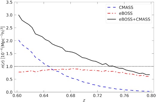
Redshift distribution of the eBOSS DR16 (red dash-dotted line), CMASS DR12 (blue dashed line), and the joint eBOSS + CMASS sample (black thick line, see Section 5.7 for details), optimized using wFKP weights.
A fibre could not be placed on 4 per cent of the LRG targets due to fibre-collisions: when a group of two or more galaxies are closer than 62 arcsec, they cannot all receive a fibre because of hardware limitations. We use PIP weights wPIP together with angular upweighting (Bianchi & Percival 2017; Percival & Bianchi 2017) to correct for this effect, as described in Mohammad et al. (2020), and Section 3.2. The final combined weight applied to the galaxies is defined as wtot = wnozwsyswFKP, and we also use wPIP applied to pairs.
The eBOSS sample of LRGs overlaps in area and redshift range with the high-redshift tail of the BOSS CMASS sample. Unlike many other eBOSS analyses including the large-scale measurements of BAO and RSD (Gil-Marín et al. 2020; Bautista et al. 2021), we do not combine the eBOSS LRG sample with all the z > 0.6 BOSS CMASS galaxies. We focus on the eBOSS sample to simplify the correction of the small-scale fibre assignment: fibre assignment was performed separately for BOSS and eBOSS using different configurations of the SDSS tiling code.
3 METHODS
3.1 Measurements
The modelling of the 3D correlation function in equation (2) is complicated by the large number of separation bins. Indeed, this requires a very large number of survey realizations to estimate the data covariance matrix. We follow the standard technique of compressing the information contained in the full 3D correlation function |$\xi \left(\boldsymbol{s}\right)$|. In particular, we fit our model to the projected correlation function wp(rp) and the first two even multipole moments ξℓ of the redshift space correlation function.
We bin rp and s in nine logarithmically spaced bins between |$0.1\text{--}60\, h^{-1}{\rm Mpc}$|, matching the output of aemulus predictions for wp(rp) and ξℓ, while the los separation π and μ are binned using linear bins of width |$\Delta \pi =1\, h^{-1}{\rm Mpc}$| and Δμ = 0.1. Given the discrete binning of different variables, we estimate the integrals in equations (3) and (4) as Riemann sums.
3.2 PIP correction
In eBOSS spectroscopic observations, fibre-collisions occur whenever two targets are closer than |$\theta ^{(\rm {fc})}=62^{\prime \prime }$| on the sky. While a fraction of such collisions are resolved thanks to multiple passes of the instruments in small chunks of the survey, fibre-collisions in single passes remain unresolved and correlate with the underlying target density. If not properly corrected, missed targets due to fibre-collisions can systematically bias the measured two-point correlation function on small scales. In the large-scale analysis of the eBOSS LRG sample (Bautista et al. 2021) fibre-collisions are accounted for by means of the nearest-neighbour (NN) weighting that is quantified through the weight wcp.
In this work, we replace the standard NN correction for fibre-collisions with a more rigorous Pairwise-Inverse-Probability (PIP) weighting (see Bianchi & Percival 2017, for a discussion about inverse-probability estimators). The PIP weights are assigned to pairs of objects in the targeted sample and quantify the probability, for any pair, of being targeted in a random realization of the survey targeting. Under the assumption that no pair has zero probability of being observed, applying the PIP weighting provides statistically unbiased estimates of the two-point correlation function. The selection probabilities are characteristic of the particular fibre assignment algorithm used to select targets from a parent photometric sample for the spectroscopic follow-up. Therefore, these probabilities are extremely difficult to model analytically except for some simple targeting strategies. We infer the selection probabilities by generating multiple replicas of the survey target selection. Details on how these survey realizations are built are provided in Mohammad et al. (2020). Given a set of survey realizations, the inverse probability, or equivalently the PIP weight wmn, is simply the number of realizations in which a given pair could have been targeted divided by the number of times it was targeted. The individual-inverse-probability (IIP) wm are the single-object counterparts of the PIP weights, i.e. the inverse-probability for a given object m of being targeted in a random survey realization.
Mohammad et al. (2020) extensively tested the effectiveness of the method of PIP + ANG weighting using a sample of 100 Effective Zel’dovich mocks (EZmocks, Zhao et al. 2021) designed to match the eBOSS LRG sample. The mean of the corrected measurements was compared to the mean of the true clustering of the mocks for ξ0, ξ2, and wp over a separation range of |$0.1\text{--}100\, h^{-1}{\rm Mpc}$| (see figs 9 and 12 of Mohammad et al. 2020). The PIP + ANG correction was able to recover the clustering of the parent sample to within 1σ of the error on the mean at all measurement scales for ξ0, and ξ2 and all scales of wp except for the fibre-collision scale, where the corrected measurements recovered the true clustering to within the error on a single mock. We can therefore be confident that the PIP + ANG correction to the eBOSS LRG sample produces unbiased results to within the statistical uncertainty of our sample on all scales.
3.3 aemulus cosmological emulator
We compare our measurements to the aemulus cosmological emulator (Zhai et al. 2019) predictions for ξ0, ξ2, and wp for a galaxy sample in a universe with variable cosmological and galaxy-halo connection parameters. The aemulus emulator applies Gaussian process based machine learning to a training set of 40 N-body simulations and that use a latin hypercube to optimally sample a wCDM parameter space spanning the approximate 4σ range of the Planck (Planck Collaboration 2020b) or WMAP (Hinshaw et al. 2013) results (DeRose et al. 2019). A halo occupation distribution model (HOD) is used to connect a galaxy sample to the dark matter haloes. Unlike some galaxy clustering analyses, our emulator does not model ξ4, since it is considerably noisier than ξ0 and ξ2. The emulator prediction would likely be noise dominated for ξ4, and would require adding more training complexity without a commensurate increase in cosmological information. In their measurement of fσ8 from small-scale clustering within the BOSS LOWZ sample, Lange et al. (2022) found that excluding ξ4 from their analysis of ξ0 and ξ2 did not produce a significant change in the best-fitting value or uncertainty.
The emulator also allows three additional parameters that control how galaxies are distributed in their host haloes: cvir, vbc, and vbs (labelled ηcon, ηvc, and ηversus in Zhai et al. 2019). cvir is the ratio between the concentration parameters of the satellites to the host halo where the halo is assumed to have a Navarro–Frenk–White (NFW) profile (Navarro, Frenk & White 1996). vbc and vbs are the velocity biases of centrals and satellites respectively, where σgal = vgalσhalo and σhalo is the velocity dispersion of the halo calculated from its mass. Finally, the aemulus emulator uses a 15th parameter, γf, which rescales all halo bulk velocities in the simulation. The galaxy velocity can therefore be thought of as the sum of two components: a component equal to the bulk motion of the host halo scaled by γf, and a randomly directed component that depends on the halo mass through the velocity dispersion and that is scaled by either vbc or vbs for centrals and satellites, respectively. For a detailed description of the aemulus correlation function parameters see Zhai et al. (2019). See Section 3.7 for a description of how we treat these parameters in our fit.
The original aemulus emulator was trained to match a BOSS CMASS-like sample at z = 0.57 and space density n = 4.2 × 10⁻⁴[h−1Mpc]−3. However, our eBOSS sample is at an effective redshift of z = 0.737 and peak number density of n = 9 × 10⁻⁵. The difference in number density is particularly worrying, since a less dense sample will preferentially fill more massive haloes. The result will be a sample with a larger linear bias, which is degenerate with the growth rate in clustering measurements. In order to ensure an unbiased result, we rebuild the emulator from the original simulations, but using the z = 0.7 simulation time-slice and adjusting HOD parameters, especially Mmin, to match the eBOSS number density. The training ranges for the new emulator are given in Table 1.
All model parameters divided into cosmological and HOD parameters, with the training range used by the aemulus emulator and the prior range used in the MCMC fit. Prior ranges were chosen to be slightly larger than the original training ranges, except where excluded by the physical meaning of the parameter, in order to be able to identify if the fit converges outside of the training range. The purpose of this extended range is only to more easily identify a prior dominated fit, since the emulator is not expected to produce accurate clustering outside of the training range. Instead, it would regress to the mean prediction. The exception is log Mcut, where the prior excludes the lower part of training range since log Mcut ceases to have any impact on the halo occupation if it is below log Mmin. This is the case for the eBOSS LRG sample, so log Mcut is poorly constrained. However, we found the chains tended to pile up at the lower end of the training range, which gave the misleading impression that the data strongly preferred the lowest possible value, although it had no effect on the cosmological constraints. For that reason, we set a more reasonable lower limit on log Msat for our sample.
| Parameter | Training range | Prior range |
|---|---|---|
| Ωm | [0.255, 0.353] | [0.225, 0.375] |
| Ωbh2 | [0.039, 0.062] | [0.005, 0.1] |
| σ8 | [0.575, 0.964] | [0.5, 1] |
| h | [0.612, 0.748] | [0.58, 0.78] |
| ns | [0.928, 0.997] | [0.8, 1.2] |
| Neff | [2.62, 4.28] | 3.046 |
| w | [–1.40, –0.57] | –1 |
| log Msat | [14.0, 16.0] | [13.8, 16.2] |
| α | [0.2, 2.0] | [0.1, 2.2] |
| log Mcut | [10.0, 13.7] | [11.5, 14] |
| σlog M | [0.1, 1.6] | [0.08, 1.7] |
| vbc | [0, 0.7] | [0, 0.85] |
| vbs | [0.2, 2.0] | [0.1, 2.2] |
| cvir | [0.2, 2.0] | [0.1, 2.2] |
| γf | [0.5, 1.5] | [0.25, 1.75] |
| fmax | [0.1, 1] | [0.1, 1] |
3.4 Interpreting growth rate measurements
As shown in Reid et al. (2014), which used a similar parametrization to measure RSD from their simulations, in the linear regime a fractional change in γf is proportional to a fractional change in f, such that f = γffΛCDM, where fΛCDM is the linear growth rate for a flat ΛCDM cosmology specified by the model parameters. However, the link between the linear velocity power spectrum amplitude and the non-linear regime is possibly scale dependent i.e. a linear response on large scales might not necessarily lead to a linear response on small scales. γf is introduced in the simulations as a scaling of all velocities by the same amount and so γf also scales the non-linear velocities of haloes. In this case, γf still provides a consistency test with the amplitude of the velocity field expected in a ΛCDM universe with the model cosmology, where γf = 1 indicates agreement, but it no longer necessarily gives a pure rescaling of the linear growth rate. For models that do have such a linear response, then the measurement of γf over the full range of scales can be used to constrain the linear growth rate. However, as this is model dependent, we conservatively separate the contributions of the linear and non-linear regime in presenting our results (as described in Section 4.1).
Although the aemulus code uses γf to adjust the RSD amplitude in the model, the RSD are sensitive to the parameter combination fσ8. We therefore present our large-scale results in terms of fσ8 = γffΛCDMσ8, which is used in the remainder of the paper and the abstract. It is also important to note that we calculate fΛCDMσ8 from the model cosmology according to linear theory, rather than the value that would be obtained from the power spectrum on scales corresponding to |$0.1\text{--}60 \, h^{-1}{\rm Mpc}$|. Thus, the value of fσ8 we present is the value expected from linear theory for our model, and is directly comparable to measurements made on larger scales. However, care should be taken when using the resulting measurements of fσ8 to constrain models where the other parameters deviate significantly from flat ΛCDM and general relativity (ΛCDM + GR, hereafter used interchangeably with ΛCDM). A problem inherent in many cosmological measurements and all previous RSD measurements is that one assumes various features of a particular model, here flat ΛCDM, in order to make the measurements. To test a different model, one should strictly have to perform a new fit including all properties of that model. This does not affect the validity of our measurement as a test of consistency with ΛCDM within the parameter space of the emulator, or as an indication of how the RSD measurements compare to those from other surveys.
3.5 Covariance matrix
Clustering measurements in different separation bins are correlated, and we need an estimate of the covariance matrix when fitting a model to the observations. Mock surveys, either based on the output of N-body simulations or approximate methods, have been widely used to estimate the data covariance matrix. However, in order to work on small scales, we would need a large number of simulations that accurately reproduce the small-scale clustering – a difficult task. In order to generate a covariance matrix that reflects the small-scale clustering of our sample, we instead use jackknife sampling. We split our survey footprint into equal area squares on the sky using right ascension (RA) and declination (Dec.) cuts. This method relies on the clustering of the sample being uncorrelated with position in the survey. Furthermore, because we expect the covariance to follow a simple volume scaling, we remove the squares with the smallest occupation as determined from the random catalogue over the survey footprint, so that each region included will contribute approximately the same statistical weight to the sampling (Fig. 2). Since the measurements from each sample are normalized, it is not necessary that they contain identical numbers of objects, however selecting regions in this way reduces variance from regions at the edge of the survey which are only partially filled or have peculiar geometries. The missing area is included in the final calculation by means of a volume-weighted correction.
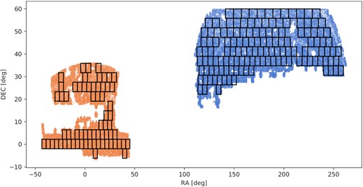
The footprint of the eBOSS LRG clustering catalogue with our jackknife regions. The blue points show the North Galactic Cap (NGC) observations, while the orange points show the South Galactic Cap (SGC) observations. It should be noted that the square jackknife regions all have approximately equal area on the sky, however due to the distortion of projecting a sphere on to a plane, the regions at larger declination appear wider in this plot.
The correlation matrix is highly diagonal, which is expected since we have a small number of widely separated bins, which are only expected to be weakly correlated. In order to reduce the noise in the off-diagonal terms, we smooth the correlation matrix using diagonally adjacent bins. Each off-diagonal element is assigned the average of itself and the two adjacent diagonal elements, excluding bins from other measurements. The result of this diagonal smoothing is shown in Fig. 3.
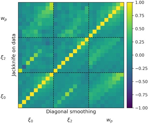
Comparison of the unsmoothed and smoothed correlation matrices. The upper diagonal elements correspond to the unsmoothed jackknife correlation matrix, while the lower diagonal elements show the result of our diagonal smoothing method.
In addition to the data error, we include the emulator error in the covariance matrix. The emulator error is calculated as a fractional error on each correlation function bin using a sample of test HOD parameter sets which are selected from the same parameter ranges as the training sample, but were not used in the training (Zhai et al. 2019). The fractional error is converted to an absolute error, σE, by multiplying by the correlation function measurements from the data. The total variance for each measurement bin is then calculated from |$\sigma _T^2=\sigma _D^2+\sigma _E^2$|. In order to preserve the structure of the jackknife covariance matrix, we convert the smoothed correlation matrix back to the covariance matrix using |$C_{i,i}=\sigma _{T,i}^2$|. The contributions of the data and emulator errors to the total error are shown in Fig. 4. The data error is dominant in the region |$s\lt 5\, h^{-1}{\rm Mpc}$| for the monopole and projected correlation function, while the emulator error is comparable for |$s\gt 5\, h^{-1}{\rm Mpc}$| and across the full separation range of the quadrupole.
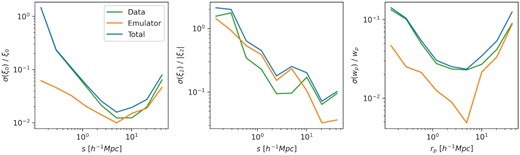
The contributions of the data error calculated through jackknife sampling (green), the emulator error (orange), and total error (blue), for the monopole, quadrupole, and projected correlation function (left- to right-hand panel).
3.6 AP scaling
The accuracy of this method depends, in part, on the width of the bins used due to the calculation of the derivative and the interpolation between points. In order to assess the importance of these factors, we perform an additional fit to the data without the AP correction. See Section 5.6 for details.
3.7 Exploring the likelihood
We assume our correlation function measurements are drawn from a multivariate Gaussian distribution, and use uniform priors for all model parameters, given in Table 1. We explore the posterior surface for the fit between data and the aemulus correlation function predictions using a Markov chain Monte Carlo (MCMC) sampler within the Cobaya2 framework (Torrado & Lewis 2021). We include the full aemulus HOD parameter space in our fit, however, we limit the wCDM cosmological parameter space by fixing Neff = 3.046 and w = −1, since these parameters are not well constrained by our measurements but have been well measured by other probes.
A concern for our small-scale analysis is that the separation range we use lacks a distinctive feature with a known scale to constrain the cosmological parameters, such as the BAO bump in large-scale analyses. Consequently, we consider a number of additional cosmological priors in order to set an accurate cosmology for our analyses. To begin with, we apply a uniform prior on the cosmological parameters based on the distance in 7D cosmological parameter space between the chain point and the cosmologies of the aemulus simulations used to train the emulator. If the distance is above a certain threshold the proposed step is forbidden, thus restricting the parameter space to the region which is well sampled by the training data, rather than the full uniform prior range given in Table 1. In practice, the main impact of the training prior is to add the restriction σ8 > 0.65, since there is only one training cosmology with σ8 below that range.
4 ROBUSTNESS AND SYSTEMATIC ERROR CHECKS
In this section, we explore the robustness of our model in general and to several possible sources of systematic error in particular. We begin by assessing the impact of non-linear velocities on our measurements, and what information is included from different scales. We then perform a general check of our method by fitting to measurements made on a mock catalogue. Finally, we check the impact of the two possible discrepancies between our model and the data, the effects of galaxy selection on the completeness of the HOD model, and redshift uncertainty.
4.1 Contribution of non-linear velocities
In Section 3.4, we introduced the key parameter of our measurement, γf, and described its significance on linear and non-linear scales. In order to identify the transition between these regimes, we examine how the emulator prediction changes for various values of γf, shown in Fig. 5. For the three largest bins, varying γf produces an almost constant relative change in the monopole, with a larger growth rate giving a larger clustering amplitude, as expected from linear theory. In the middle three bins, the effect on the monopole changes signs as the quasi-linear regime transitions to the non-linear regime, where the random virial motions of the haloes begin to dominate and increasing γf, which rescales all halo velocities, begins to damp the clustering. In the three smallest bins, the effect of γf on the monopole begins to decrease as the one-halo term begins to dominate. Because γf affects only the halo velocities, and in our HOD formalism, we do not assign galaxies based on subhalos, varying γf has no effect on the one-halo term. Motivated by this result, we divide our nine measurement bins into three groups of three bins, with individual ranges of |$0.1\text{--}0.8\, h^{-1}{\rm Mpc}$|, |$0.8\text{--}7\, h^{-1}{\rm Mpc}$|, and |$7\text{--}60\, h^{-1}{\rm Mpc}$|. These three ranges correspond roughly to the strongly non-linear regime where the one-halo term is dominant, the transition between the non-linear and quasi-linear regimes, and the quasi-linear regime. We therefore restrict our measurement of fσ8 to the quasi-linear regime, where γf can be interpreted as a rescaling of the linear growth rate. For measurements performed over the full separation range, we instead use γf as a test of ΛCDM, where a deviation from γf = 1 indicates that the velocity field of the data as parametrized by our emulator model is in disagreement with the expectation from ΛCDM.
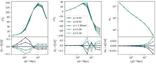
The effect on the emulator prediction of varying γf for the monopole (left-hand panel), quadrupole (centre hand panel), and projected correlation function (right-hand panel). All other parameters are kept fixed at reasonable values for the baseline eBOSS fit. Upper panels: Direct comparison of the predictions, ranging from low γf (blue) to high γf (red). Lower panels: Relative difference to the γf = 1 prediction.
4.2 Galaxy selection and the HOD model
As described in Section 3.3, we add an additional parameter fmax to the emulator compared to previous uses that controls the maximum occupation fraction of central galaxies in the HOD framework, in order to address the incompleteness of the eBOSS LRG sample due to target selection. We test the necessity of this addition and the effect on the clustering using a series of HOD mock galaxy catalogues. We constructed these mocks from the Uchuu3 simulation. Briefly, Uchuu is a |$(2000 \, h^{-1}{\rm Mpc})^3$|, 128003 particle simulation using the Planck2015 cosmology and a mass resolution of |$m_p=3.27\times 10^8 \, h^{-1}M_\odot$|. We construct the mocks from the z = 0.7 slice, using the halotools4 (Hearin et al. 2017) python package and an HOD parametrization identical to that outlined in Section 3.3. We constructed mocks using σlog M, log Msat, α, and log Mcut from five randomly selected test HOD parameter sets in aemulus, with log Mmin tuned to give n = 1 × 10⁻⁴. The aemulus test HOD sets are themselves randomly selected from the uniform training range given in Table 1, but were not used in training the emulator. In all mocks, we kept the additional parameters vbc = 0, vbs = 1, cvir = 1, and γf = 1 fixed to their simplest, no scaling values. For each of the five HOD parameter sets, we then constructed five mocks with fmax = [0.2, 0.4, 0.6, 0.8, 1.0], for a total of 25 mocks.
We fit these 25 HOD mocks using two emulators: one matching the original aemulus HOD model that is equivalent to fixing fmax = 1, and the full emulator with variable fmax. Both emulators were built to match the eBOSS redshift and number density, as described in Section 3.3. The γf constraints on the HOD mocks from both emulators are shown in Fig. 6, where the expected value is γf = 1 by the construction of the mocks. It should be noted that all of the mocks were constructed using the same halo catalogue from a single simulation box at a particular cosmology, so it is unsurprising that the constraints do not scatter evenly above and below γf = 1, since they are not fully independent. The key points to notice are that the variable fmax emulator is able to recover the expected value of γf within the uncertainty over the full fmax range, and shows no trend in fmax. Conversely, the fixed fmax emulator shows a clear bias in γf for fmax ≤ 0.6. This result matches what we would theoretically expect for model which overestimates the fmax value of the sample. If the mismatch is small, there is not a significant change in the galaxy bias of the sample, however if fmax is significantly overestimated then the model prediction has a larger galaxy bias, b, than the sample, which is compensated by a lower growth rate since the amplitude of the linear clustering scales as fb2.
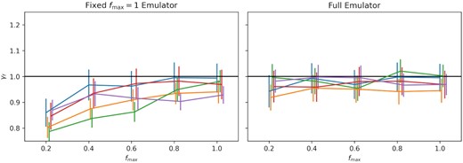
Performance of emulators with fixed or variable fmax on HOD mocks constructed with varying fmax. The left-hand panel shows the results from an emulator built with the original aemulus parameter set, which is equivalent to fmax = 1. The right-hand panel shows the results from the emulator used in our analysis with variable fmax. Both emulators were built to match the eBOSS redshift and number density. The horizontal line shows the expected value of γf used to construct the mocks. Points are shifted slightly along the x-axis to avoid overlap.
4.3 Redshift uncertainty
Another area of concern where the emulation based model may not accurately reflect the data is the effect of redshift uncertainties. As shown in Fig. 2 of Ross et al. (2020), the eBOSS LRG sample has a redshift uncertainty that is well approximated by a Gaussian with mean |$\mu =1.3\rm ~km~s^{-1}$| and standard deviation |$\sigma =91.8\rm ~km~s^{-1}$|. On average, this means that each redshift is wrong by an absolute offset of |$65.6 \rm ~km~s^{-1}$|. To first order this gives a Gaussian random velocity shift for all targets, which acts to damp the clustering of the multipoles on small scales. The parameters vbc and vbs, which control the velocity dispersion of centrals and satellites, respectively, should be able to mimic much of this effect in the model without affecting the constraints on other parameters. However, since γf scales all halo velocities in the simulation, on non-linear scales where the halo velocities are virialized, γf has a similar effect on the clustering as the redshift uncertainty, vbc and vbs. In addition, vbc and vbs are both calculated by scaling the virial dispersion of the host halo, so the galaxy velocities derived in the model have a mass dependence which is not reflected in the redshift uncertainty. The result is that the redshift uncertainty may bias the recovered value of γf on non-linear scales, with an unmodelled redshift uncertainty giving a larger than expected value of γf.
We test the effect of the redshift uncertainty on the γf and fσ8 constraints using a second set of HOD mocks, constructed in the same way as those described in Section 4.2. We selected 25 new aemulus test HOD parameter sets and generated HOD catalogues using halotools. We then calculated the clustering with and without a random velocity shift along the los drawn from a Gaussian with mean |$\mu =1.3\rm ~km~s^{-1}$| and standard deviation |$\sigma =91.8\rm ~km~s^{-1}$|. The change in the measured values of γf from the full separation range and fσ8 from the quasi-linear scales only (matching the method used for our baseline results) due to the inclusion of the random velocity shift are shown in Fig. 7. For all 25 mocks, including a random velocity shift increased the value of γf measured from the full separation range, with an average shift slightly greater than half the statistical uncertainty. The larger value of γf measured due to the random velocity shift matches our theoretical expectation for the degeneracy between γf and the redshift uncertainty on non-linear scales, and the magnitude of the shift indicates that the redshift uncertainty is a significant concern when fitting to the non-linear scales. On the other hand, the shifts in the measured value of fσ8 scatter around 0, with a mean shift over an order of magnitude smaller than the statistical uncertainty. This result also agrees with what is expected for our model, since on quasi-linear scales the redshift uncertainty is not degenerate with a change in γf, and instead will change only vbc and vbs. Therefore, the redshift uncertainty is not a concern for our value of fσ8 measured from the quasi-linear scales.
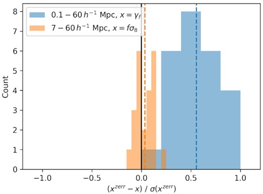
A histogram of the shifts in the measured cosmological parameters for 25 HOD mocks with and without a random velocity dispersion matching the eBOSS redshift uncertainty. Blue bars show the shift in γf measured over the full separation range, and orange bars show the shift in fσ8 measured from the quasi-linear scales only. The x-axis shows the difference between the value measured for the mock with a random velocity dispersion (zerr) and the value measured from the same mock without the additional velocity dispersion, divided by the uncertainty of the measurement from the zerr mock. Coloured dashed lines show the mean shift for each case. For the fit over |$0.1\text{--}60\, h^{-1}{\rm Mpc}$|, including a random velocity dispersion not represented in the model increased the measured value of γf for all 25 mocks, with a mean shift slightly larger than half of the statistical uncertainty. Conversely, for the fit over |$7\text{--}60\, h^{-1}{\rm Mpc}$|, the shifts from including a random velocity dispersion scatter around 0, with a mean shift that is negligible compared to the statistical error.
There are several barriers to including a correction for the redshift uncertainty in the model. Most significantly, the redshift uncertainty grows with redshift (see fig. 6 of Bolton et al. 2012 for BOSS redshift evolution), while the emulator is constructed from catalogues at a single redshift slice. The evolution with redshift is also important because the eBOSS LRG targeting cuts were made using the apparent magnitudes of the targets, so properties of the sample such as the mean mass will also evolve weakly with redshift and correlate with the growth of the redshift uncertainty. The result is that including the redshift uncertainty in the model may not be as simple as drawing from a uniform velocity shift, and would require more detailed testing and corrections. The effect of redshift uncertainty could instead be included as an additional systematic error or shift in our measured values. However, it is important to note that for every mock tested, the inclusion of redshift uncertainty (without it being present in the model) increased the measured value of γf, because on the non-linear scales where the redshift uncertainty is the most significant, it is degenerate with the larger random motions of the haloes provided by a larger value of γf. In Section 5, we consistently measure values of γf that are below the value expected from ΛCDM + Planck2018, so the presence of redshift uncertainty is actually expected to increase this tension rather than lowering it. We therefore take the conservative approach of excluding a shift in our measurements due to the redshift uncertainty, even though it would be expected to increase the tension shown by our measurements, and leave a complete treatment of the redshift uncertainty to future work.
4.4 SHAM mocks
We test the robustness of our model and analysis pipeline using a subhalo abundance matching (SHAM) mock generated from the Uchuu simulation. By using a SHAM mock rather than a HOD mock, we remove the dependence on the specific galaxy-halo connection model used in our analysis, providing the best approximation to a model independent test. If our analysis is able to correctly recover the expected value of γf = 1 for the SHAM mock, then we can be confident it will be able to match the data, even if there are deviations from the specific functional form of the galaxy–halo connection model described in Section 3.3. We use the z = 0.7 slice of the simulation to construct a SHAM mock using the peak halo velocity, Vpeak, with a scatter of 0.2 dex, and a number density of n = 1 × 10⁻⁴ in order to match the eBOSS LRG number density and redshift.
The result of our fit to the SHAM mock is shown in Fig. 8. The primary purpose of the Uchuu SHAM mock test is to assess the robustness of the cosmological parameter recovery using our HOD based emulator, so we have only included the parameters which have the greatest impact on the γf constraint. The constraints on all of the cosmological parameters are in good agreement with the known values from the simulation, and the 1D marginalized constraint on γf is γf = 0.964 ± 0.049, which agrees to within 1−σ with the known value of γf = 1 for the mock. All well constrained HOD parameters converge within the training parameter space indicating that the emulator is able to accurately model the clustering of the mock, despite the mock being constructed using a different galaxy–halo connection. This result shows that are analysis pipeline and model provide robust constraints on the growth rate.
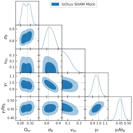
Two dimensional and one dimensional marginalized constraints of the key parameters from the fit to an Uchuu SHAM mock matching the eBOSS LRG number density and redshift. Dotted lines show the values of the cosmological parameters from the simulation.
5 RESULTS
In this section, we present the results of our fit to the small-scale LRG clustering. We also investigate the robustness of our results by testing the inclusion of additional constraints on the cosmological parameters, examining how the constraints change depending on which scales and measurements are included in the analysis, the effect of covariance matrix smoothing on the measured parameters, and consistency with the constraints from a combined CMASS + eBOSS sample.
5.1 Headline results
We fit the eBOSS LRG monopole, quadrupole, and projected correlation function over scales |$0.1\lt r\lt 60\, h^{-1}{\rm Mpc}$| using the Cobaya MCMC sampler. We restrict the cosmological parameter space using the aemulus training prior described in Section 3.7, but do not include any external data. We obtain a value of γf = 0.767 ± 0.052, 4.5σ below what would be expected in a ΛCDM + GR universe. The 1D and 2D likelihood contours of the full parameter set are shown in Fig. 9. All well constrained parameters are within the prior ranges described in Table 1, and the parameters that are most impactful for our results, Ωm, σ8, vbc, and γf, all show roughly Gaussian constraints. The best-fitting values of the cosmological parameters other than γf are consistent with recent measurements from the Planck Collaboration (Planck Collaboration 2020b). The best-fit model prediction is plotted relative to the data in Fig. 10, showing reasonable agreement within the measurement uncertainty on all scales. The best-fitting prediction has χ2 = 14.1, with 14 degrees of freedom and 27 data points, indicating a good fit. In addition, we consider a fit over only the quasi-linear scales of our measurements, |$7\text{--}60\, h^{-1}{\rm Mpc}$| as described in Section 4.1, from which we obtain a value of fσ8(z = 0.737) = 0.408 ± 0.038. This value is 1.4σ below what is expected from the 2018 Planck data for a flat ΛCDM universe, and is a factor of 1.7 improvement in statistical error over the more standard large-scale analysis of the same data set. See Section 5.4 for more details.
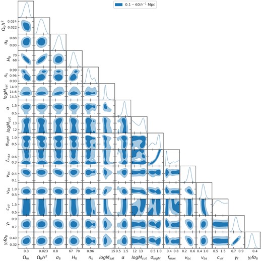
One dimensional and two dimensional contours of the parameters used in our baseline fit, as well as the derived constraints on γffσ8.
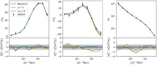
Comparison of the best-fitting model predictions to the data several fit to the eBOSS LRG sample for the monopole (left-hand panel), quadrupole (centre panel) and projected correlation function (right-hand panel). Upper panels: the baseline fit (blue), fixed γf = 1 fit (orange), and vbc = 0 fit (green), with the data and measurement uncertainty (black). Lower panels: The difference between the best-fitting models and the data divided by the measurement uncertainty. The 1 − σ region is shown in grey.
5.2 Testing the quasi-linear scales for overfitting
One concern for our fit to the quasi-linear scales is that by reducing the separation range to |$7\text{--}60\, h^{-1}{\rm Mpc}$|, we are fitting nine data points with a 14 free parameter model. However, it is important to note that many of the HOD parameters have a negligible effect on these scales. In particular, the three parameters that control the satellite occupation (log Msat, α, log Mcut) and the three parameters that control the positions of galaxies in the haloes (vbc, vbs, cvir) have very little impact and are almost entirely constrained by the |$0.1\text{--}7\, h^{-1}{\rm Mpc}$| bins. Therefore, while there are 14 free parameters in the model, only eight are significant when fitting to the nine bins of the quasi-linear scales. While this provides a theoretical explanation for why the quasi-linear scales will not be overfit, our fit over the scales |$7\text{--}60\, h^{-1}{\rm Mpc}$| has a minimum χ2 = 0.36 (Table2), indicating that the small scale HOD parameters may still be causing some overfitting.
γf constraints with statistical errors calculated from the width of the 1D marginalized posterior and χ2 values for the fits used in our analysis. NP gives the number of free model parameters in the fit and ND gives the number of data points. *The eBOSS + Planck18 runs jointly fit 5 of the 14 parameters with Planck, so they are not fully independent.
| Run | γf | NP | ND | χ2 |
|---|---|---|---|---|
| |$0.1\text{--}60\, h^{-1}{\rm Mpc}$| | 0.767 ± 0.052 | 14 | 27 | 14.1 |
| |$0.1\text{--}7\, h^{-1}{\rm Mpc}$| | 0.71 ± 0.14 | 14 | 18 | 7.8 |
| |$0.8\text{--}60\, h^{-1}{\rm Mpc}$| | 0.783 ± 0.066 | 14 | 18 | 4.2 |
| |$7\text{--}60\, h^{-1}{\rm Mpc}$| | 0.854 ± 0.083 | 14 | 9 | 0.36 |
| |$7\text{--}60\, h^{-1}{\rm Mpc}$|, eight parameters | 0.821 ± 0.064 | 8 | 9 | 0.74 |
| |$7\text{--}60\, h^{-1}{\rm Mpc}$|, six parameters | 0.802 ± 0.050 | 6 | 9 | 1.8 |
| ξ0 + ξ2 | 0.819 ± 0.073 | 14 | 18 | 5.0 |
| ξ0 + wp | 0.65 ± 0.11 | 14 | 18 | 5.4 |
| γf = 1 | 1 | 13 | 27 | 28.0 |
| vbc = 0 | 0.958 ± 0.088 | 13 | 27 | 22.5 |
| fmax = 1 | 0.764 ± 0.051 | 13 | 27 | 16.6 |
| Unsmoothed covariance matrix | 0.767 ± 0.052 | 14 | 27 | 14.3 |
| Scaled mock covariance matrix | 0.766 ± 0.059 | 14 | 27 | 12.0 |
| No training prior | 0.85 ± 0.12 | 14 | 27 | 12.1 |
| eBOSS + Planck18 | 0.784 ± 0.048 | 14* | 27 | 18.5 |
| eBOSS + Planck18 scaled σ8 | 0.798 ± 0.047 | 14* | 27 | 19.1 |
| eBOSS + Planck18 free σ8 | 0.766 ± 0.053 | 14* | 27 | 18.0 |
| No AP scaling | 0.772 ± 0.053 | 14 | 27 | 14.5 |
To test if this overfitting affects our results, we perform additional fits over the |$7\text{--}60\, h^{-1}{\rm Mpc}$| separation range with the predominantly small scale HOD parameters fixed to their best-fitting values from the fit over the full |$0.1\text{--}60\, h^{-1}{\rm Mpc}$| separation range. In the first additional fit we keep the six parameters listed above fixed, leaving eight parameters (Ωm, Ωbh2, σ8, h, ns, σlog M, γf, fmax) free. In the second fit, we also keep σlog M and fmax fixed to their best-fitting values from the full fit, allowing only the six cosmological parameters to vary. The γf constraints from these fits are shown in Table 2 and Fig. 11. The results of both fits show that reducing the parameter space increases the precision of the γf constraint without significantly shifting the central value, while increasing the minimum χ2. We conclude that allowing the small scale HOD parameters to be free does lead to the quasi-linear scales being overfit, however, it does not bias our cosmological constraints and instead only increases the uncertainty. Fixing these HOD parameters would increase the precision of our measurement from the quasi-linear scales, but it would also introduce an indirect dependence on the non-linear scales. We therefore take the conservative choice of using the measurement with all 14 parameters free as our baseline result. However, this test does show the value of including the non-linear scales in a measurement of the linear growth rate.

γf constraints from all the runs listed in Table 2. The blue point shows the baseline fit to the full separation range, extended by the blue dashed line for comparison to other points. The red point shows the fit to the quasi-linear scales only. The black dashed line shows γf = 1 for comparison, the value expected if the amplitude of the halo velocity field matches the ΛCDM expectation.
5.3 Testing the impact of the cosmological priors
We consider a number of prior constraints on the cosmological parameters, as described in Section 3.7. The three most significant cases are a uniform prior as described in Table 1, a uniform prior that restricts the cosmological parameters to be within the volume that is well sampled by the training simulations, and a joint fit with Planck2018 likelihoods with a scaled value of σ8 to account for the redshift difference between the data and the model. The constraints on the key parameters for these three prior choices are shown in Fig. 12. The parameter that is most significantly impacted by the prior choice is σ8, with all three methods giving consistent values but with large differences in precision. However, the constraint on fσ8 is almost unchanged for all prior choices. This result clearly shows the robustness of the fσ8 fit from the data, and demonstrates the freedom of the model where changes in σ8 can be balanced by γf. It is also important to note that because the uncertainty on fσ8 is dominated by the uncertainty of γf that the training prior and the joint fit with Planck achieve almost the same precision on fσ8, despite having comparable constraints on γf but a significant difference in precision on σ8.
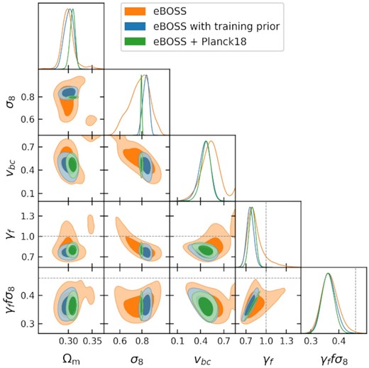
One dimensional and two dimensional contours of the key fit parameters for the fit to the eBOSS LRG sample with no additional cosmological constraints (orange), restricted by the aemulus training prior (blue), and jointly fit with the Planck2018 likelihoods (green).
The effect of the three treatments of σ8 for the joint Planck fit described in Section 3.7 can be found in Table 2. Using the same value of σ8 for the Planck chains and model, scaling to account for the redshift offset, or excluding the Planck constraints on σ8 all give consistent values for the growth rate, again demonstrating the robustness of the fit.
5.4 Testing the dependence on the data fitted
In order to test the consistency of the constraint on γf from the different regimes described in Section 4.1, we fit to the full non-linear regime (|$0.1\text{--}7\, h^{-1}{\rm Mpc}$|), the weakly non-linear and quasi-linear regimes (|$0.8\text{--}60\, h^{-1}{\rm Mpc}$|), and the quasi-linear regime only (|$7\text{--}60\, h^{-1}{\rm Mpc}$|). One dimensional and two dimensional contours in the vbc − γf parameter space for these three fits are shown in the left-hand panel of Fig. 13. There is little variation in the other parameters between these fits to different scales, however some important insight is gained from examining the vbc − γf degeneracy since both parameters have a similar effect on the clustering in the non-linear regime. The fits to smaller scales yield larger and more precise values of vbc, while obtaining smaller and less precise constraints on γf. The full fit to all scales is located at the intersection in vbc − γf space of the small and larger scale fits. The result is that there is mild tension between the constraints on small and large scales, although the significance when considering the combined uncertainty is less than 1 − σ. It is worth recalling that since γf rescales all halo velocities in the simulation, in the linear regime it can be used to derive a constraint on the linear growth rate fσ8, in the non-linear it also enhances the effects of non-linear growth. So the fit to the small-scales is really a consistency check between the data and model with ΛCDM, and these results showing that there is a strong tension which is most significant in the non-linear regime.
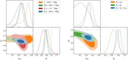
Two dimensional and one dimensional marginalized constraints on vbc and γf for fits to different scales and measurements. Left-hand panel: constraints from the three largest separation bins (orange), six largest separation bins (green), six smallest separation bins (red), and all nine separation bins (blue) for all three measurements. The dotted line shows γf = 1, the value expected if the amplitude of the halo velocity field matches the expectation from ΛCDM. Right-hand panel: constraints from the joint fit to the monopole and projected correlation function (orange), monopole and quadrupole (green), and all three measurements (blue).
The fit to the quasi-linear scales only does not show the same degeneracy between vbc and γf since they no longer have the same effect on the clustering, and is broadly consistent with any value of vbc since it ceases to be impactful on such large scales. However, the large scale fit is still able to recover a relatively tight constraint on γf that can be compared directly to the linear growth rate, giving a measurement fσ8 = 0.408 ± 0.038, which is 1.4σ lower than the value expected from the 2018 Planck data for a flat ΛCDM model.
We also examine the effect of excluding certain measurements from the fit. In the right-hand panel of Fig. 13, we show the constraints in vbc − γf parameter space from the joint fit to only the monopole and projected correlation function, and the joint fit to the multipoles only. The multipole only fit is less sensitive to the degeneracy between vbc and γf, but prefers a smaller value of vbc and larger γf compared to the full fit. On the other hand, the joint fit of the monopole and projected correlation function, which contain similar clustering information but are sensitive and insensitive to the effects of RSD respectively, prefer a non-zero value of vbc with much greater confidence, compensated by a low but less well constrained value of γf. As with the fits to different scales, the full fit lies in the overlap region produced by the different sensitivities of these measurements.
5.5 Testing the dependence on the covariance matrix
The results of the fits using this scaled mock covariance matrix and the original unsmoothed jackknife covariance are shown in Table 2. The constraints in both cases are nearly identical to our baseline fit using the smoothed jackknife covariance matrix, indicating that our analysis is robust to the choice of covariance matrix.
5.6 Testing the dependence on AP correction
We test the dependence of our result on the AP correction by running a full fit excluding the AP correction. The constraint on γf from this fit can be seen in Table 2 and Fig. 11. Excluding the AP correction has a negligible effect on the constraint on γf and slightly increases the best-fitting χ2. We therefore conclude that any uncertainty in the AP correction due to the large bin width and approximate calculation will not have a significant effect on our cosmological constraints.
5.7 Including the BOSS CMASS data
We test the reliability of our fit using a combined CMASS + eBOSS sample in the redshift range 0.6 ≤ z ≤ 0.8. In particular, in our analysis we use the CMASS sample from the DR12 data release. The CMASS DR12 catalogue covers an area of |$9376\deg ^2$| over a redshift range of 0.4 < z < 0.8 (Reid et al. 2016) with a target density of |$99.5\deg ^{-2}$|. The target selection is calibrated to provide a sample of galaxies with approximately constant stellar mass over the spanned redshift range. We refer the reader to Reid et al. (2016) for a detailed description of the target selection and properties for CMASS sample. In order to perform a joint measurement of the two-point correlation function using the eBOSS and CMASS catalogues, we restrict the two samples (and the corresponding random catalogues) only to the area of the sky where they overlap and to the redshift range of 0.6 < z < 0.8. The redshift distributions of the two samples as well as their joint distribution are shown in Fig. 1.
The advantage of this sample is that it is more complete due to the complimentary nature of the CMASS and eBOSS colour cuts. However, the inclusion of the additional CMASS objects skews the redshift distribution of the sample, which is not ideal for an HOD-based analysis where the galaxy–halo connection parameters are implicitly assumed to be the same across the full redshift range of the sample, and several are dependent on the density of galaxies. As such, we use our combined CMASS + eBOSS measurement to provide a consistency check with our fit, particularly our assumption that the target selection of eBOSS does not affect our measurement, but we continue to use the eBOSS only constraint as our fiducial measurement.
To correct fibre-collisions in the CMASS sample, we use a modified version of the NN upweighting with completeness correction, designated CP, as described in section 2.3 of Mohammad et al. (2020), and the standard angular upweighting method described in Section 3.2. For the eBOSS LRG sample, the CP correction was found to perform similarly to the PIP only result on all scales of wp, ξ0, and ξ2 (see figs 15 and 18 of Mohammad et al. 2020). Given the similarities in sample type and targeting between CMASS and eBOSS, it is reasonable to expect a similar result for CMASS. When combined with angular upweighting, any systematic bias is expected to be below the statistical uncertainty of the measurement. Since our primary goal in analyzing the combined CMASS + eBOSS sample is as a consistency check, this correction is sufficient for our purposes.
Fig. 14 shows the result of our fit compared to the eBOSS only fit in the most important parameters of our analysis for both the full emulator range and the quasi-linear scales only. The CMASS + eBOSS measurement is consistent with the eBOSS only measurement in all parameters, although there is a greater preference for larger fmax values, as expected. It is interesting to note that in the fit over the full emulator range the inclusion of the CMASS data does not affect our γf constraint, including not reducing the 1D marginalized uncertainty. However, there are several reasons why including additional data may not reduce 1D marginalized constraints. First, the additional data may reduce the allowed parameter space in 14 dimensions without affecting the 1D constraints on a specific parameter. Additionally, the uncertainty in our measurement is limited by the emulator accuracy in several bins, notably the quadrupole and the large scale bins of the monopole and wp, so a reduction of measurement uncertainty in these bins will not be reflected in the fit. Finally, the constraint on γf seems to rely on the complimentary constraining of different scales and probes on parameter combinations such as vbc and γf (Fig. 13). The fit to CMASS + eBOSS has slightly less tension between the small and large scales than the eBOSS only measurement, so the overlap region remains the same size even though the uncertainty from separated scales has been reduced. This can be seen in the fit to the quasi-linear scales, where the combined CMASS + eBOSS sample gives a constraint of fσ8 = 0.384 ± 0.036. This constraint is consistent with the eBOSS only measurement from the quasi-linear scales, but because it is slightly lower, it is in less tension with the fit over the full separation range.
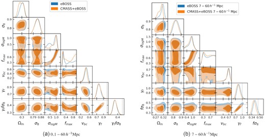
Two dimensional and one dimensional marginalized constraints of the key parameters of our fit for our fiducial eBOSS measurement (blue) and combined CMASS + eBOSS sample (orange). The two plots show (a) the fit over the full emulator range, and (b) the fit to the quasi-linear scales only.
6 DISCUSSION
6.1 Comparison to other measurements
We compare our result to other measurements of fσ8 from galaxy clustering surveys in Fig. 15. Taken as a whole sample, there is clearly good consistency with the ΛCDM prediction. For the eBOSS LRGs, Bautista et al. (2021) analyzed pairs with separations between |$25\text{--}130\, h^{-1}{\rm Mpc}$|, and obtained measurements of fσ8 = 0.446 ± 0.066 and 0.420 ± 0.065 depending on the RSD model used in the analysis (see Table B1 of Bautista et al. 2021). Our measurement is consistent with these results at around the 1 − σ level, but has a factor of 1.7 improvement in the statistical error. Our measurement also continues the trend of galaxy clustering measurements of fσ8 falling slightly below the prediction from observations of the CMB.
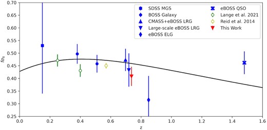
fσ8 measurements from various SDSS samples. The blue points show the results of the standard large-scale analyses from the SDSS MGS (Howlett et al. 2015), BOSS galaxies (Alam et al. 2017), CMASS + eBOSS LRGs, eBOSS LRGs (Bautista et al. 2021), eBOSS ELGs (de Mattia et al. 2021), and eBOSS quasars (Neveux et al. 2020). Our small-scale analysis of the eBOSS LRGs using only the quasi-linear regimes is shown in red. Empty coloured points show the results of small-scale analyses from the BOSS LOWZ sample (Lange et al. 2022, green) and BOSS CMASS sample (Reid et al. 2014, yellow) that included non-linear scales in the analysis. The black line shows the expected value of fσ8 for a flat ΛCDM universe with the best-fitting Planck2018 cosmology. The large-scale eBOSS LRG result is shifted in the x-axis to avoid overlap with the small-scale result from this work.
In Fig. 15, we also compare our results to other attempts to measure fσ8 on small scales. Reid et al. (2014) used a similar parametrization as our analysis to measure fσ8 from the small-scale clustering of the BOSS CMASS sample, and achieved the highest precision to date. However, due to the difficulty of modelling the non-linear regime Reid et al. (2014) used a fixed cosmology, which has been shown by Zhai et al. (2019) to significantly reduce the uncertainty. Conversely, Lange et al. (2022) use a novel modelling method in their analysis of the BOSS LOWZ sample that does not require an emulator. It should also be noted that their model does not include an equivalent of our γf parameter that allows the linear growth rate to change independently of the ΛCDM cosmology. Both of these analyses have split in linear and non-linear regimes differently than our analysis, which significantly affects the claimed uncertainty. By restricting our measurement of fσ8 to only the quasi-linear scales, our uncertainty increases by a factor of ∼1.5 compared to our fit over the full |$0.1\text{--}60\, h^{-1}{\rm Mpc}$| separation range, however, we can be confident that what we are measuring is purely the linear growth rate, and so can be directly compared to other more standard large-scale measurements. As shown in Sections 5.1 and 5.4, using the full separation range significantly increases the tension with the result expect for ΛCDM, with the non-linear scales in greater disagreement with the expected value than the quasi-linear scales, however it is no longer clear if this tension arises from a discrepancy in the linear growth rate or a difference in the non-linear velocity field measured in the data using the emulator model.
It is interesting to note that Lange et al. (2022) found a similar dependence on the measurement scales, with smaller scales preferring a smaller value of fσ8. Lange et al. (2022) also found that adding the projected correlation function to their fiducial measurement of the monopole, quadrupole, and hexadecapole reduced the best-fitting value of their lower redshift sample by 1 − σ, but did not significantly affect the measurement from their higher redshift sample. Differences between the two analysis methods mean it is expected that there would be some variation in the impact of the different measurements and scales between our results. This is particularly true since Lange et al. (2022) do not include a parameter comparable to our γf, given the importance of wp in breaking the vbc − γf degeneracy in our analysis.
6.2 Galaxy–halo connection parameters
The parameter found to be most degenerate with our γf constraint is vbc, the scaling of the velocity dispersion of centrals in the HOD framework (Fig. 9). A lower value of vbc corresponds to a larger γf, as expected in the non-linear regime since both parameters increase the observed velocity dispersion of galaxies (see Section 4.3). Our fit over the full |$0.1\text{--}60 \, h^{-1}{\rm Mpc}$| separation range strongly prefers a non-zero vbc and low γf. However, our fit to the quasi-linear regime finds no discernible degeneracy between vbc and γf and recovers both a relatively large value of γf and non-zero value of vbc, although the constraint on vbc is weak to the small impact it has on those scales (Fig. 13). This result indicates that the degeneracy between vbc and fσ8 may illustrate the degree to which the non-linear scales affect the overall constraint. Lange et al. (2022) also find a strong degeneracy between the velocity scaling of central galaxies and their constraint on fσ8, with their higher redshift sample yielding vbc > 0 and low fσ8 compared to the ΛCDM prediction. Reid et al. (2014) elected to fix the velocity of centrals to match that of the host halo, and find closer agreement with the ΛCDM expectation, which we also find when using a fixed vbc = 0. vbc > 0 indicates that a central galaxy is in motion relative to the centre of the host halo, either because the central galaxy is oscillating in the potential or because the system is not fully relaxed. Understanding the physical processes that would lead to this effect, especially if the process is redshift dependent, will be important for future analyses.
We also investigate the dependence of our measurement on the fmax parameter. Due to the strong degeneracy between σlog M and fmax, our fit to the data is broadly consistent with a wide range of values for fmax between 0.2 and 1, however there is a large peak at fmax = 0.25. A low value of fmax is not surprising for the eBOSS sample given the magnitude and colour cuts made when selecting the target sample, particularly since the highest magnitude objects were removed. We do not find a degeneracy with fσ8, so the lack of constraint on σlog M and fmax is not expected to bias our measurement.
Numerical simulations have shown that the clustering of dark matter haloes can depend on properties other than halo mass, a.k.a halo assembly bias (Sheth & Tormen 2004; Gao, Springel & White 2005; Harker et al. 2006; Wechsler et al. 2006; Obuljen, Dalal & Percival 2019). This bias can propagate into the distribution of galaxies that live in these haloes and thus introduce additional bias in the clustering measurement. In the analysis of BOSS galaxies over a wider redshift range Zhai et al. (2022), we enhance the basic HOD approach used here with an assembly bias model depending on the environment of dark matter haloes. Although the results of that analysis imply the mild existence of assembly bias, there is a negligible impact on the cosmological constraint and measurement of structure growth rate. Therefore, we exclude explicit modelling of assembly bias in this paper.
6.3 Comparison to tension from lensing surveys
It is interesting to note that we obtain a lower value of fσ8 than expected from Planck measurements, given the current σ8-tension between Planck and weak lensing surveys and the low amplitude of the galaxy–galaxy lensing amplitude measured using the BOSS CMASS sample by Leauthaud et al. (2017), since both tensions could be resolved by a lower value of σ8 than that measured by Planck. To see approximately how our result might relate to this tension, we compare the constraints on S8 = σ8(ΩM/0.3)0.5 for the DES Y1 results (Abbott et al. 2018), Planck 2018 (Planck Collaboration 2020b), and our results (Fig. 16). The left-hand panel shows our measurement using the full separation range, while the right-hand panel shows our measurement from the quasi-linear scales only. Our constraint, shown as the blue contour, is consistent with both the DES Y1 and Planck results in both cases. However, it is important to note that our low value of fσ8 comes almost entirely from γf < 1, which reduces the magnitude of peculiar velocities in the simulation without affecting the amplitude of fluctuations, σ8. If the low value of fσ8 we measure was due to the value of σ8 instead then the constraint would shift down the S8 axis, shown as a green contour. For our measurement from the quasi-linear scales this shift maintains consistency with both DES Y1 and Planck 2018, however for our fit to all scales this shift puts the green constraint in tension with the Planck results, and in more mild disagreement with the DES results. This result may indicate that the increased tension we find from the non-linear scales may be caused by an issue with the HOD model, rather than a purely cosmological tension.
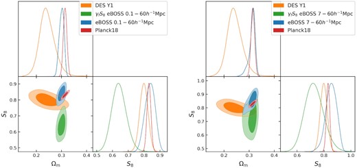
Two dimensional and one dimensional marginalized constraints on Ωm and S8 from our analysis (blue), the Dark Energy Survey (DES) year 1 results (Abbott et al. 2018) (orange) and Planck 2018 results (Planck Collaboration 2020a, c) (red). Since our low value of fσ8 mostly comes from γf, we also plot γfS8 (green) for our fit, which shows the constraint we would have if the low value of fσ8 came entirely from the σ8 value. Left-hand panel: results of our full fit to all scales. Right-hand panel: results from only the quasi-linear scales used to constrain the linear growth rate.
6.4 Emulator robustness and potential improvements
We have performed rigorous tests of the emulator performance (see Section 4), and found that the model performs well when fit to an independent simulation and galaxy–halo connection prescription. We also find that a model that assumes all central galaxies are observed leads to a systematic bias in the recovered cosmological parameters if the actual fractional occupation of centrals is lower than 0.6. We correct this bias by adding the parameter fmax to the emulator, and verify that the full emulator gives an unbiased measurement for 0.2 < fmax < 1.0. We also identify the redshift uncertainty as a source of systematic bias on non-linear scales, with a redshift uncertainty missing from the model leading to an offset in γf to larger values by more than half of the statistical error for the eBOSS sample. This is a significant concern for future small-scale analyses, and will require careful attention due to the difficulties in implementing a redshift dependent effect in a model constructed at a single redshift. The redshift uncertainty has also been found to scale with redshift, so it will be an even greater concern for future large surveys at high redshift such as DESI (DESI Collaboration 2016a, b) and Euclid (Laureijs et al. 2011).
Our measurement of the clustering within the eBOSS LRG sample also meets or exceeds the emulator precision in several of the measurement bins (see Fig. 4), showing the importance of improving the model precision for future surveys. This must be balanced against ensuring there are sufficient bins to yield a well defined fit, given the number of model parameters (see Section 5.2). Finally, careful attention must be given to the non-linear scales, and identifying what information can be used to constrain the linear growth rate. A key aspect includes ensuring the performance of the HOD model on these scales, and investigating the effect of baryonic physics.
7 SUMMARY
We have measured the growth rate of structure from the small-scale clustering of the eBOSS LRG sample corrected by PIP weights and modelled using the aemulus cosmological emulator. Using the quasi-linear scales of our measurement range, we obtain a measurement of fσ8(z = 0.737) = 0.408 ± 0.038, which is 1.4σ lower than the value expected from 2018 Planck data for a flat ΛCDM model. Our measurement is a significant improvement over more standard measurements made using only the large-scale modes, achieving a level of precision that is 1.7 times better than the large-scale analysis of the same sample. Using the full separation range of our measurement, we find a 4.5σ tension in the amplitude of the halo velocity field with the expectation for a ΛCDM universe. This tension is driven by the non-linear scales of our analysis and so may not be well modelled by a change in the linear growth rate, but may instead reflect a breakdown in the HOD model used in the emulator.
We perform a robust check of possible sources of systematic error not included in previous analyses. We find that using a model that assumes all central galaxies are observed leads to a systematic bias if the actual occupation of centrals is lower; a fractional occupation of fmax ≤ 0.6. We also investigate the effect of redshift uncertainty, and find that the presence of a velocity shift from redshift uncertainty in the data that is not included in the model results in a higher measurement of γf with an offset of ∼0.5σ, where σ is the typical statistical error. This effect is caused by the degeneracy between the increased velocity dispersion due to the redshift uncertainty and the random motions of the haloes in the non-linear regime. Lastly, we investigate the consistency between the non-linear and quasi-linear scales of our analysis. While we find them to be consistent within the statistical error, there is a trend to lower γf on non-linear scales, which increases the tension with the expectation from ΛCDM for the fit to all scales. This result highlights the importance of distinguishing between results obtained from the linear scales and thus directly constraining the linear growth rate fσ8, and those that include non-linear scales and may have a non-linear dependence on the linear growth rate together with a dependence on other factors.
While our results are consistent with the expectation from Planck 2018 parameter constraints, we are also consistent with recent weak lensing results giving a low value of S8, particularly if our low value of fσ8 was driven by an adjustment to σ8. In light of these lensing results and the mild disagreement we find with Planck expectations, extending this type of analysis to future surveys including DESI and Euclid will be an important area of future research. With considerably larger samples and probing a different redshift range, the improvement in precision from moving to smaller scales will be key to achieving optimal constraints and identifying or rejecting a tension in the growth rate of cosmic structure.
ACKNOWLEDGEMENTS
ZZ is supported in part by NASA grant 15-WFIRST15-0008, Cosmology with the High Latitude Survey Roman Science Investigation Team (SIT). JLT acknowledges the support of NSF AAG grant 2009291. MJC, FGM, ZZ, and WJP acknowledge financial support from the Canadian Space Agency (CSA) and the Natural Sciences and Engineering Research Council of Canada (NSERC). GR acknowledges support from the National Research Foundation of Korea (NRF) through Grants Nos 2017R1E1A1A01077508 and 2020R1A2C1005655 funded by the Korean Ministry of Education, Science and Technology (MoEST).
Research at Perimeter Institute is supported, in part, by the Government of Canada through the Department of Innovation, Science and Economic Development Canada and by the Province of Ontario through the Ministry of Colleges and Universities.
This research was enabled, in part, by the support provided by Compute Ontario (www.computeontario.ca) and Compute Canada (www.computecanada.ca).
Funding for the Sloan Digital Sky Survey IV has been provided by the Alfred P. Sloan Foundation, the U.S. Department of Energy Office of Science, and the Participating Institutions. SDSS-IV acknowledges support and resources from the Center for High Performance Computing at the University of Utah. The SDSS website is www.sdss.org. SDSS-IV is managed by the Astrophysical Research Consortium for the Participating Institutions of the SDSS Collaboration including the Brazilian Participation Group, the Carnegie Institution for Science, Carnegie Mellon University, Center for Astrophysics | Harvard & Smithsonian, the Chilean Participation Group, the French Participation Group, Instituto de Astrofísica de Canarias, The Johns Hopkins University, Kavli Institute for the Physics and Mathematics of the Universe (IPMU) / University of Tokyo, the Korean Participation Group, Lawrence Berkeley National Laboratory, Leibniz Institut für Astrophysik Potsdam (AIP), Max-Planck-Institut für Astronomie (MPIA Heidelberg), Max-Planck-Institut für Astrophysik (MPA Garching), Max-Planck-Institut für Extraterrestrische Physik (MPE), National Astronomical Observatories of China, New Mexico State University, New York University, University of Notre Dame, Observatário Nacional / MCTI, The Ohio State University, Pennsylvania State University, Shanghai Astronomical Observatory, United Kingdom Participation Group, Universidad Nacional Autónoma de México, University of Arizona, University of Colorado Boulder, University of Oxford, University of Portsmouth, University of Utah, University of Virginia, University of Washington, University of Wisconsin, Vanderbilt University, and Yale University.
DATA AVAILABILITY
The eBOSS galaxy and random catalogues are publicly available at: https://data.sdss.org/sas/dr16/eboss/lss/catalogs/DR16/ with a description here: https://www.sdss.org/dr16/spectro/lss/ We used the aemulus emulator, which is available here: https://aemulusproject.github.io, and the cobaya package, which is available here: https://github.com/CobayaSampler.
Footnotes
Available at github.com/desihub/redrock
Cobaya, a code for bayesian analysis in cosmology, is the python successor to CosmoMC. Users are able to use the same MCMC sampler as CosmoMC (Lewis & Bridle 2002; Lewis 2013) in a python framework, while allowing access to likelihoods from many major cosmological datasets. The sampler is tailored for parameter spaces with a speed hierarchy and implements the ‘fast dragging’ procedure described in Neal (2005). See https://cobaya.readthedocs.io for details.
