


ABSTRACT
We present cosmological constraints from the analysis of angular power spectra of cosmic shear maps based on data from the first three years of observations by the Dark Energy Survey (DES Y3). Our measurements are based on the pseudo-Cℓ method and complement the analysis of the two-point correlation functions in real space, as the two estimators are known to compress and select Gaussian information in different ways, due to scale cuts. They may also be differently affected by systematic effects and theoretical uncertainties, making this analysis an important cross-check. Using the same fiducial Lambda cold dark matter model as in the DES Y3 real-space analysis, we find |${S_8 \equiv \sigma _8 \sqrt{\Omega _{\rm m}/0.3} = 0.793^{+0.038}_{-0.025}}$|, which further improves to S8 = 0.784 ± 0.026 when including shear ratios. This result is within expected statistical fluctuations from the real-space constraint, and in agreement with DES Y3 analyses of non-Gaussian statistics, but favours a slightly higher value of S8, which reduces the tension with the Planck 2018 constraints from 2.3σ in the real space analysis to 1.5σ here. We explore less conservative intrinsic alignments models than the one adopted in our fiducial analysis, finding no clear preference for a more complex model. We also include small scales, using an increased Fourier mode cut-off up to |$k_{\rm max}={5}\, {h}\, {\rm Mpc}^{-1}$|, which allows to constrain baryonic feedback while leaving cosmological constraints essentially unchanged. Finally, we present an approximate reconstruction of the linear matter power spectrum at present time, found to be about 20 per cent lower than predicted by Planck 2018, as reflected by the lower S8 value.
1 INTRODUCTION
Gravitational lensing by the large-scale structure coherently distorts the apparent shapes of distant galaxies. The measured effect, cosmic shear, is sensitive to both the geometry of the Universe and the growth of structure, making it, in principle, a powerful tool for probing the origin of the accelerated expansion of the Universe and, consequently, the nature of dark energy. After the first detections two decades ago (Bacon, Refregier & Ellis 2000; Kaiser, Wilson & Luppino 2000; Van Waerbeke et al. 2000; Wittman et al. 2000), methodological advances in measurement algorithms were permitted by newly collected data, e.g. from the Deep Lens Survey (DLS; Wittman et al. 2002; Jee et al. 2013, 2016), the COSMOS survey (Scoville et al. 2007), the Canada–France–Hawaii Telescope Legacy Survey (CFHTLS; Semboloni et al. 2006) and Canada–France–Hawaii Telescope Lensing Survey (CFHTLenS; Joudaki et al. 2017) and the Sloan Digital Sky Survey (SDSS; Huff et al. 2014). These were fostered by community challenges (see e.g. Heymans et al. 2006; Massey et al. 2007; Bridle et al. 2009; Kitching et al. 2012; Mandelbaum et al. 2014). Ongoing surveys, such as the Dark Energy Survey1 (DES; Flaugher 2005), the ESO Kilo-Degree Survey2 (KiDS; de Jong et al. 2013; Kuijken et al. 2015), and the Hyper Suprime-Cam Subaru Strategic Program3 (HSC; Aihara et al. 2018a, b), have produced data sets capable of achieving cosmological constraints that are competitive with cosmic microwave background observations on the amplitude of structure, σ8, and the density of matter, Ωm, through the parameter combination |$S_8\equiv \sigma _8\sqrt{\Omega _{\rm m}/0.3}$| (Troxel et al. 2018; Hikage et al. 2019; Hamana et al. 2020, 2022b; Planck Collaboration VI 2020; Asgari et al. 2021; DES Collaboration 2022). These surveys are paving the way for the next generation of surveys, namely the Vera Rubin Observatory Legacy Survey of Space and Time4 (LSST; Ivezić et al. 2019), the ESA satellite Euclid5 (Laureijs et al. 2012), and NASA’s Nancy Grace Roman Space Telescope6 (Akeson et al. 2019), which will improve upon current observations in quality, area, depth, and spectral coverage, in the hope of better determining the nature of dark energy. However, the level of precision needed to fully exploit the cosmological information contained in these future observations pushes the community to dissect every component of the analysis framework, from data collection to inference of cosmological parameters.
The two-point statistics of the cosmic shear field are most commonly used to extract cosmological information. While it is well known that the shear or convergence fields are, to some extent, non-Gaussian (Springel, Frenk & White 2006; Yang et al. 2011), i.e. that there is information in higher order statistics (e.g. in peaks, Dietrich & Hartlap 2010; Martinet et al. 2018; Jeffrey, Alsing & Lanusse 2021a; Harnois-Déraps et al. 2021; Zürcher et al. 2021, or three-point functions, Takada & Jain 2003; Fu et al. 2014), the two-point functions remain the primary source of information, as they can be predicted by numerical integration of analytical models (Zuntz et al. 2015; Joudaki et al. 2017; Chisari et al. 2019; Krause et al. 2021) and efficiently measured (Jarvis 2015). The shear two-point function can be characterized by its two components, ξ+(θ) and ξ−(θ), as a function of angular separation θ, or by its Fourier (or harmonic) counterpart, the shear angular power spectrum, Cℓ, as a function of multipole ℓ (with an approximate mapping ℓ ∼ π/θ). Both have been measured on recent data from the DES (DES Year 1; Troxel et al. 2018; Camacho et al. 2021; Nicola et al. 2021, and DES Year 3, Amon et al. 2022; Secco, Samuroff et al. 2022), KiDS (KiDS-450; Hildebrandt et al. 2017; Köhlinger et al. 2017, and KiDS-1000, Asgari et al. 2021; Loureiro et al. 2021), and HSC (Hikage et al. 2019; Hamana et al. 2020, 2022b).
While, in principle, the two statistics summarize the same information, practical considerations require discarding some of the measurements for cosmological analyses via scale cuts. As a consequence, the information retained by the two statistics differs in practice, which introduces some statistical variance in cosmological constraints, on top of potential differences due to differential systematic effects. Indeed, constraints reported for the analyses of cosmic shear with KiDS-450 data showed a difference between the real- and harmonic-space analyses of ΔS8 = 0.094 (Hildebrandt et al. 2017; Köhlinger et al. 2017), and that of HSC Year 1 data a difference of Δσ8 = 0.24 and ΔS8 = 0.045 (Hikage et al. 2019; Hamana et al. 2020, 2020a, b), both corresponding to about 2σ discrepancies (see also Fig. 11, discussed below). More recently, the comparison between three different estimators presented for KiDS-1000 data, on the other hand, showed excellent agreement (Asgari et al. 2021), including a newly developed pseudo-Cℓ estimator in Loureiro et al. (2021). In a preparatory study (Doux et al. 2021), we quantified this effect for DES Y3 by means of simulations and showed (i) that the difference on the S8 parameter is expected to fluctuate by about σ(ΔS8) ∼ 0.02 for typical scale cuts, and (ii) that the observed difference is the result of the interplay between scale cuts and systematic effects, and how these impact each statistic.
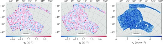
Maps of the two shear components, γ1 and γ2, and density, ng, of the full DES Y3 weak lensing catalogue.

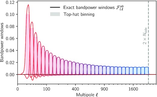
Bandpower window functions |$\mathcal {F}_{L\ell }^{ab}$| from equation (15). Each curve corresponds to one of the 32 bandpowers L from ℓmin = 8 to ℓmax = 2Nside = 2048, which are equally spaced on a square-root scale throughout this work. The naive binning function is shown by the filled histogram behind.
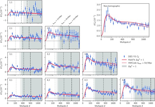
Cosmic shear power spectra measured from DES Y3 data. Each panel in the lower left triangle corresponds to a redshift bin pair indicated in the upper left corner. The measured E-mode component of the binned, noise-bias corrected power spectra is shown in blue with error bars from an analytical covariance matrix (see Section 3.3). The grey shaded regions show scales that are not used in the fiducial analysis (Δχ2 = 1) where the effect of baryons is neglected, with extra points removed when combining with shear ratios shown in light grey (see Section 3.5.1). The corresponding best-fitting model within ΛCDM, discussed in Section 6.1, is represented by red solid lines. The grey dashed lines show the scale cuts corresponding to kmax = 1, 3, and 5 |$h\, {\rm Mpc}^-1$| (see also Section 3.5.2), and the corresponding best-fitting model using hmcode and |$k_{\rm max}={5}\, {h}\, {\rm Mpc}^{-1}$|, discussed in Section 6.3, is represented by red dashed lines. The upper right panel shows the measured non-tomographic shear power spectrum of DES Y3 data in blue, along with the theory expectation corresponding to the best fit of the tomographic analysis, in red. For readability, all measurements and errors bars are scaled by the mean multipole |$\bar{L}$| of each bandpower L, i.e. the data points show |$\bar{L}\hat{{\bf C}}_L^{EE}$| and are compared to theoretical predictions of ℓCℓ.
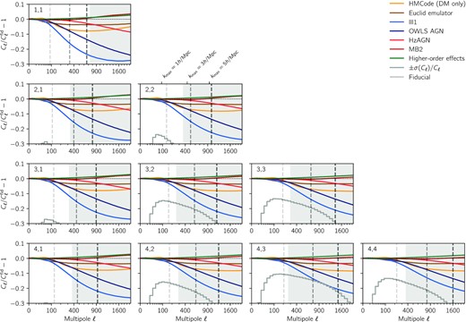
Residual shear power spectra with respect to the fiducial power spectra, |$C_\ell ^{\rm fid}$|. The orange (hmcode) and brown (euclid emulator) curves show residuals for alternative prescription of the non-linear power spectrum (see Section 3.2.2). The blue and red curves show the effect of baryons as predicted by four hydrodynamical simulations (Illustris, OWLS AGN, Horizon AGN, and MassiveBlack II). Higher order lensing effects computed with CosmoLike are also shown, in green, to be small. The error bars are shown by the grey step-wise lines which represent ±σ(Cℓ)/Cℓ on the same scale (only −σ(Cℓ)/Cℓ is visible). The grey-shaded regions show scales that are not used in the fiducial analysis where the effect of baryons is neglected. The grey dashed lines show the scale cuts corresponding to kmax = 1, 3, and 5 |$h\, {\rm Mpc}^{-1}$|(see Section 3.5.2).
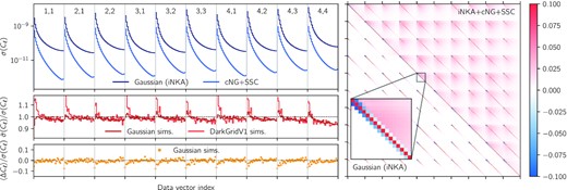
Features and validation of the analytical covariance matrix used in this work, computed with namaster and cosmolike. Upper left: error bars given by the square-root of the diagonal of the Gaussian (dark blue) and non-Gaussian (light blue) contributions to the covariance matrix. Middle left: comparison of the error bars computed from Gaussian simulations (dark red) and darkgridV1 simulations (light red) with the fiducial error bars. Lower left: residuals of the pseudo-Cℓ measurements from the Gaussian simulations with respect to the input (binned) spectra. In all left-hand panels, the horizontal axis corresponds to indices of the components stacked data vector. The corresponding redshift bin pairs are indicated at the top of the upper panel, with each block corresponding to multipoles in the range 8–2048. Right: correlation matrix, with only the Gaussian contribution in the lower triangle, and both Gaussian and non-Gaussian contributions in the upper triangle (note the normalization in the range −0.1 to +0.1).
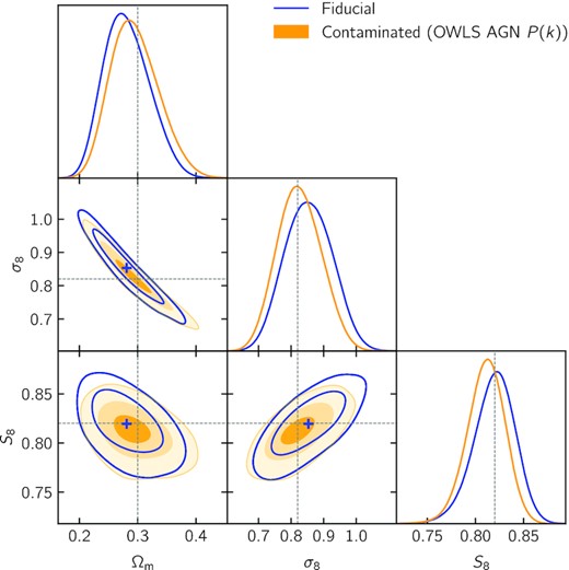
Validation of the Δχ2 < 1 scale cuts. We compare constraints from a noiseless data vector produced at the fiducial cosmology (dark blue) to those obtained from a contaminated data vector obtained by rescaling the matter power spectrum using equation (25) with the OWLS AGN simulation, both using the fiducial model. The nested, filled regions show the 0.3σ, 1σ, and 2σ contours, corresponding to roughly 24, 68, and 95 per cent confidence regions. The mean of the fiducial posterior, which is represented by the blue plus sign, lies within the 0.3σ contour of the contaminated posterior.
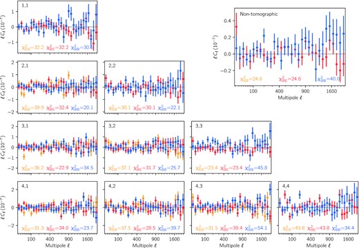
EB and BB cosmic shear power spectra measured with DES Y3 data for each pair of tomographic bins in the lower triangle, and the entire sample in the upper right panel (note that the EB and BE power spectra are different only for cross-redshift bin spectra). Error bars are computed from 10 000 Gaussian simulations using the DES Y3 catalog ellipticities and positions, as explained in Section 4.1.1. We find a χ2 of 344.0 for 320 degrees of freedom for tomographic B-mode power spectra, corresponding to a probability-to-exceed of 0.17. We find a χ2 of 535.4 for 512 degrees of freedom for EB tomographic cross-power spectra (counting all 16 independent bin pairs), corresponding to a probability-to-exceed of 0.23. Individual χ2 are reported for each redshift bin pairs in the corresponding panels. In the non-tomographic case, we find, for the B-mode power spectrum, a χ2 of 40.0 for 32 degrees of freedom, corresponding to a probability-to-exceed of 0.16.
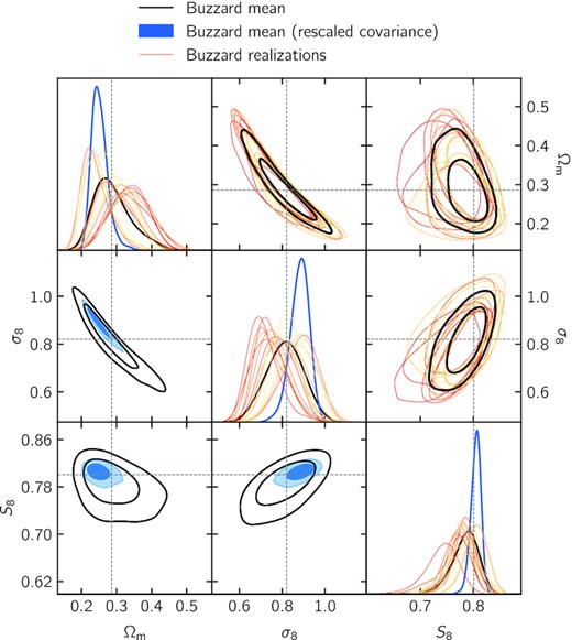
Validation of the analysis framework with Buzzard simulations. We show the 1D and 2D marginal posterior distributions corresponding to the mean Buzzard data vector with the data covariance (black) and the same covariance rescaled by a factor 1/16 (blue). The posteriors obtained for each realization are shown in yellow to red.
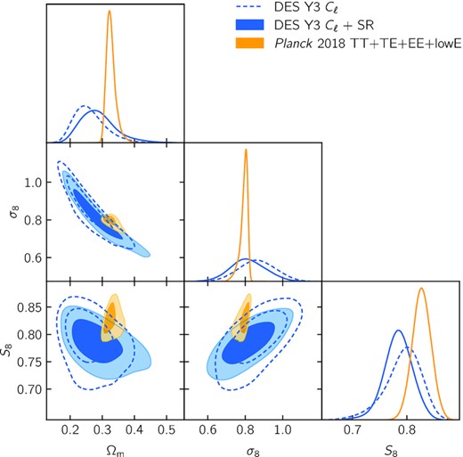
Cosmological constraints on the amplitude of structure σ8, the total matter density Ωm and their combination |${S_8\equiv \sigma _8\sqrt{\Omega _{\rm m}/0.3}}$|. The inner (outer) contours show 68 per cent (95 per cent) confidence regions. Constraints from DES Y3 cosmic shear power spectra with the two sets of fiducial scale cuts are shown in blue, with (solid) and without (dashed) shear ratios (Sánchez et al. 2021). Constraints obtained from Planck2018 measurements of cosmic microwave background temperature and polarization anisotropies are shown in yellow (Planck Collaboration VI 2020).
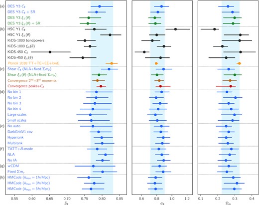
Comparison of 1D marginal posterior distributions over the parameters S8 ≡ σ8(Ωm/0.3)0.5, σ8 and Ωm, from DES Y3 data as well as other experiments, and consistency tests for this work (in blue). (a) Constraints obtained from the harmonic (this work) and real (Amon et al. 2022; Secco et al. 2022) space analyses of DES Y3 data are shown in blue and green (see also Fig. 14), both with and without shear ratio information (SR; Sánchez et al. 2021). (b) Constraints from other weak lensing surveys, namely HSC Y1 (Hikage et al. 2019; Hamana et al. 2020, 2022b), KiDS-1000 (Asgari et al. 2021), and KiDS-450 (Hildebrandt et al. 2017; Köhlinger et al. 2017) are shown in grey, and constraints from cosmic microwave background observations from Planck 2018 are shown in yellow (Planck Collaboration VI 2020). (c) Constraints from four weak lensing analyses of DES Y3 data are compared, including the analysis of mass map moments (Gatti et al. 2021b) and peaks (Zürcher et al. 2022), and illustrating a high level of consistency (see also Fig. 15). (d) Consistency tests where redshift bins are removed one at a time (first four) and where the data vector is split into its large- and small-scale data points (last two) (see also Appendix C). (e) Various other consistency tests: removing autopower spectra, swapping the covariance matrix, and marginalizing over redshift distribution uncertainties with HyperRank and MultiRank(see also Appendix C). (f) Modelling robustness test for intrinsic alignment (IA), including B-mode power spectra, or replacing TATT by NLA, or removing IA contributions altogether (see also Section 6.2, Fig. 12). (g) Other robustness test, freeing the dark energy equation-of-state w or fixing the neutrino mass to 0.06 eV. (h) Baryonic feedback tests where the matter power spectrum is computed with HMCode instead of HaloFit, and fiducial scale cuts are replaced with kmax = 1, 3, and 5 |$h\, {\rm Mpc}^{-1}$| scale cuts (see also Section 6.3 and Fig. 13).
In this work, we present measurements of (tomographic) cosmic shear power spectra measured from data based on the first three years of observations by the Dark Energy Survey (DES Y3), which we use to infer cosmological constraints on the ΛCDM model. We then extend our analysis and vary scale cuts to derive constraints on intrinsic alignments and baryonic feedback at small scales, the two largest astrophysical sources of uncertainty on cosmic shear studies (Chisari et al. 2018; Mandelbaum 2018; Secco et al. 2022). Finally, we study the consistency of these constraints with those inferred from other DES Y3 weak lensing analyses, using two-point functions (Amon et al. 2022; Secco et al. 2022) and non-Gaussian statistics (Gatti et al. 2021b; Zürcher et al. 2022).
The paper is organized as follows: Section 2 presents DES Y3 data; Section 3 introduces the formalism relevant to the estimation of cosmic shear power spectra and the cosmological model, including systematic effects, intrinsic alignments and baryonic feedback; Section 4 highlights the different tests we performed to validate both the measurement and modelling pipelines, some of which rely on simulations (Gaussian, N-body, and hydrodynamical); Section 5 details the three-step blinding procedure we adopted in this work; Section 6 presents our main results, i.e. cosmological constraints inferred from the analysis of DES Y3 cosmic shear power spectra, and compares them to other weak lensing studies; and finally Section 7 summarizes our results.
2 DARK ENERGY SURVEY YEAR 3 DATA
The Dark Energy Survey The Dark Energy Survey Collaboration (DES, 2005) is a photometric imaging survey that covers around 5000 square degrees of the Southern hemisphere in five optical and near-infrared bands (grizY). Its observations were carried out at the Cerro Tololo Inter-American Observatory (CTIO) in Chile, using the 570-megapixel DECam camera mounted on the Blanco telescope (Flaugher et al. 2015), during a six-year campaign (2013–2019). This work is based on data collected during the first three years (Y3) of observations, in particular the DES Y3 weak lensing shape catalogue presented in Gatti et al. (2021c), which is a subsample of the Y3 Gold catalogue (Sevilla-Noarbe et al. 2021), and the inferred redshift distributions presented in Myles et al. (2021).
2.1 Shape catalogue
Galaxy shape calibration biases are usually parametrized in terms of multiplicative and additive components. The DES Y3 shape measurements are based on the metacalibration algorithm, which allows to self-calibrate most shear multiplicative biases, including selection effects, by measuring the response of the shape measurement pipeline to an artificial shear (Huff & Mandelbaum 2017; Sheldon & Huff 2017). The residual multiplicative biases, at the 2–3 per cent level, are dominated by shear-dependent detection and blending effects, and the correction was measured on a suite of realistic, DES-Y3-like image simulations presented in MacCrann et al. (2022).
The shape catalogue was validated by a series of (null) tests presented in Gatti et al. (2021c) and found to be robust to both multiplicative and additive biases. The fiducial DES Y3 catalogue used here comprises ellipticity measurements for 100204026 galaxies, with inverse-variance weights based on signal-to-noise ratio and size. The effective area of the sample is 4143 deg2 (see Sevilla-Noarbe et al. 2021, for details), corresponding to an effective density of |${\bar{n}={5.59}\, {\rm gal/arcmin}^2}$|. Fig. 1 shows the two ellipticity components and the density of the entire sample. We will construct similar maps for each of the four tomographic bin (see next section) and use them to measure cosmic shear power spectra.
2.2 Redshift distributions
The DES Y3 shape catalogue was further divided into four tomographic bins, based on photometric redshifts inferred with the Sompz algorithm (phenotypic redshifts with self-organizing maps, Buchs et al. 2019). The DES Y3 implementation is detailed in Myles et al. (2021) and is based on measurements in the riz bands. The g band was excluded in DES Y3 weak lensing analyses due to known issues in modelling the point spread function (Jarvis et al. 2021) required by metacalibration. This exclusion was shown to degrade estimated redshift distributions in when five tomographic bins were used (Buchs et al. 2019), motivating the use of four bins. The DES Y3 implementation of sompz thus connects DES wide-field photometry to (i) deep-field observations (Hartley et al. 2022), using image injection with the Balrog software (Everett et al. 2022), and to (ii) external spectroscopic and high-quality photometric samples, to calibrate redshifts. This Bayesian framework allows to consistently sample the posterior distribution of the four redshift distributions, while propagating calibration and sample uncertainties. Given an ensemble of realizations, uncertainties can be marginalized-over during sampling by means of the hyperrank method (Cordero et al. 2022). The initial ensemble that was generated for DES Y3 was subsequently filtered using constraints on redshifts from cross-correlations with spectroscopic samples, as detailed in Gatti et al. (2022). The residual uncertainty on the mean redshift of each tomographic bin is of the order of σ〈z〉 ∼ 0.01. Redshift distributions are shown in the upper panel of Fig. 2, where, for each bin, the ensemble mean is represented by a solid line, and the ensemble dispersion is represented by the light bands. The lensing efficiency functions corresponding to the mean distributions at the fiducial cosmology are shown in the lower panel.
3 METHODS
In this work, we aim at extracting cosmological constraints from the measurements of the angular auto- and cross-power spectra of the tomographic cosmic shear fields inferred from DES Y3 data. This section describes the estimation of angular spectra from data and the multivariate Gaussian likelihood model, including theoretical predictions for power spectra and their covariance matrix.
3.1 Angular power spectrum measurements
The formalism introduced so far is valid for a full-sky observations. In practice, however, the cosmic shear field is only sampled within the survey footprint, at the positions of galaxies. This induces a complicated sky window function, or mask, that correlates different multipoles and biases the estimators defined in equations (6) and (8). We therefore estimate angular power spectra with the so-called pseudo-Cℓ or MASTER formalism (Hivon et al. 2002) using the namaster software (Alonso et al. 2019) to correct for the effect of the mask. We provide a summary of the method here and refer the reader to Hikage et al. (2011) for the development of the pseudo-Cℓ formalism for cosmic shear, to Alonso et al. (2019) for the namaster implementation and to Nicola et al. (2021) and Camacho et al. (2021) for recent applications of the pseudo-Cℓ formalism with namaster to DES Y1 and HSC cosmic shear data.
We do not apply any purification of E and B modes (Lewis, Challinor & Turok 2001; Smith 2006; Grain, Tristram & Stompor 2009; Alonso et al. 2019) since the B-mode signal is largely subdominant and does not contain cosmological information, to first order. Moreover, this would require an apodization of the mask, that is speckled with empty pixels due to fluctuations in the density of source galaxies and small vetoed areas, and thus significantly decrease the effective survey area.
Finally, we correct for the effect of the pixelization of the shear fields into healpix maps. As noted in Nicola et al. (2021), it depends on the density of galaxies, at fixed resolution: at low density, each pixel contains at most one galaxy and the map is sampling the shear field itself (but has many empty pixels), whereas at higher density, we are estimating the average of the shear field within each pixel. Here, for a resolution of Nside = 1024, we find that pixels with at least one galaxy contain on average 17.2–17.5 galaxies for all four tomographic bins, meaning that we are indeed sampling the averaged shear field (although a small fraction of pixels, especially on the footprint edges, have only one galaxy). This is then corrected for by dividing the pseudo-spectra |$\tilde{{\bf C}}_\ell ^{ab}$| by the (squared) healpix pixel window function |$F_\ell ^2$|, or equivalently, assigning weights |$w_{L}^{\ell }=1/F_\ell ^2$| for ℓ ∈ L for measurements (except for theoretical predictions). We test the effect of the resolution parameter in Appendix C1, and verify that it has negligible impact on cosmological constraints. In Section 4, we validate these hypotheses and the measurement pipeline with Gaussian and N-body simulations.
The estimated shear power spectra for DES Y3 data are shown in Fig. 4, along with the best-fitting model for our fiducial ΛCDM results.
3.2 Modelling
In this section, we describe the theoretical model for the observed shear power spectra, including systematic uncertainties.
3.2.1 Theoretical background
3.2.2 Non-linear power spectrum
Following the general methodology of the DES Y3 large-scale structure analysis set in Krause et al. (2021), for our fiducial model we compute the non-linear matter power spectrum PNL(k, z) using the Boltzmann code camb(Lewis, Challinor & Lasenby 2000; Howlett et al. 2012) with the halofit extension to non-linear scales (Smith et al. 2003), with updates to dark energy and massive neutrinos from Takahashi et al. (2012). halofit is reported to be accurate at the 5 per cent level for |$k \le {1}\, h\, {\rm Mpc}^{-1}$|, when compared to N-body simulations, and degrading for smaller scales. However, Krause et al. (2021) showed that DES Y3 cosmic shear is insensitive to varying the prescription to model the small-scale power spectrum by substituting HaloFit for hmcode (with dark matter only), the euclid emulator, or the mira-titan emulator (Mead et al. 2015; Lawrence et al. 2017; Euclid Collaboration 2019). We show a comparison of some of these prescriptions in Fig. 5 and we verify the robustness of our fiducial choice in in Section 4.4.1.
3.2.3 Intrinsic alignments
Galaxies are extended objects and therefore subject to tidal forces. Their intrinsic shapes, or ellipticities, are consequently not fully random but rather tend to align with the tidal field of the gravitational potential and therefore each other (Hirata & Seljak 2004; Bridle & King 2007). As a consequence, the shear power spectrum estimated from galaxies receives additional contributions from the correlation of intrinsic shapes, |$C_{\ell ,{\rm I}{\rm I}}^{ab}$|, and the cross-correlations of intrinsic shapes with the cosmological shear field, |$C_{\ell ,{\rm GI}}^{ab}$| and |$C_{\ell , {\rm IG}}^{ab}$|, such that the theoretical spectrum of the observed signal reads |${C_\ell ^{ab}+C_{\ell ,{\rm GI}}^{ab}+C_{\ell , {\rm IG}}^{ab}+C_{\ell ,{\rm I}{\rm I}}^{ab}}$|.
In this work, we follow the DES Y3 analysis of cosmic shear in real space (Krause et al. 2021; Amon et al. 2022; Secco et al. 2022) and use the so-called TATT framework (Blazek et al. 2019) as our fiducial choice to model these extra terms stemming from intrinsic alignments (IA). This model unified tidal alignment (TA) with tidal torquing (TT) mechanisms, proposed by Catelan, Kamionkowski & Blandford (2001), Crittenden et al. (2001), and Mackey, White & Kamionkowski (2002), thanks to a perturbative expansion of the intrinsic galaxy shape field in the density and tidal fields, up to second order in the tidal field. We refer the reader to Secco et al. (2022) for full details of the implementation and a justification of this choice. The TA and TT contributions are each modulated by an amplitude (respectively, ATA and ATT) and a redshift-dependence parameter (respectively, αTA and αTT), with an additional linear bias bTA of sources contributing to the TA signal. The non-linear alignment model (NLA; Hirata & Seljak 2004; Bridle & King 2007), commonly used in cosmic shear analyses (Troxel et al. 2018; Hikage et al. 2019; Hamana et al. 2020, 2022b; Asgari et al. 2021) is contained in the TATT framework and corresponds to the case ATT = bTA = 0.
The TATT model also predicts a small, but non-zero B-mode power spectrum, when bTA ≠ 0 or ATT ≠ 0. In the main parts of the analysis, the B-mode spectrum is not used for cosmological analysis. Instead, it is demonstrated in Section 4.2.1 that DES Y3 data is consistent with no B modes, rejecting the hypothesis of a strong contamination of the signal by systematic effects that would source B modes, such as leakage from the PSF, measured in Section 4.2.2 and Appendix A. This test thereby also excludes a detectable contribution of the IA B-mode signal, with the unlikely caveat that systematic effects and IA may cancel each other. In addition, the PSF test allows us to predict the contamination of B-mode spectra, which is found to be subdominant, by an order of magnitude, to the TATT-predicted B-mode signal for ATT = 1, which is well within current E-mode constraints. Therefore, we will extend the cosmological analysis in Section 6.2 and include B-mode measurements to improve constraints on the TATT parameters. To do so, we employ the same pseudo-Cℓ formalism and extend the mode-coupling matrices in equations (10) and (14) to account for the B-mode component. Note that namaster computes both E and B components of the mixing matrices as well as the cross-terms accounting for leakages between the two components. The fiducial analysis simply discards those terms, as B-to-E mode leakage is found to be negligible. However, E-to-B mode leakage is found to significantly contribute to the B-mode signal, in comparison to the TATT-predicted B-mode signal (they are of comparable magnitude for ATT of order unity). Therefore, the extended analysis including B-mode measurements uses consistent modeling of multipole coupling and E/B-mode leakage. The covariance matrix for the B-mode measurement as well as the cross-covariance between E- and B-mode measurements are computed from a set of 10 000 Gaussian simulations based on DES Y3 data, as detailed in Section 4.1.1.
3.2.4 Effects of baryons
Astrophysical, baryonic processes redistribute matter within dark matter haloes and modify the matter power spectrum at small scales (Chisari et al. 2018; Schneider et al. 2019, 2020; Huang et al. 2021). Feedback mechanisms from active galactic nuclei and supernovae heat up their environment and suppress clustering in the range k ∼ 1–10 |$h\, {\rm Mpc}^{-1}$|, while cooling mechanisms enhance clustering on smaller scales. The complex physics involved in these mechanisms has been modelled in multiple hydrodynamical simulations (van Daalen et al. 2011; Dubois et al. 2014; Vogelsberger et al. 2014; Khandai et al. 2015). However, the absolute and relative amplitudes of the various effects remain poorly understood and constitute a major source of uncertainty, at the level of tens of per cent, on the matter power spectrum at scales |$k\gtrsim {5}\, {h}\, {\rm Mpc}^{-1}$|, and on the shear power spectrum at multipoles as low as ℓ ≳ 100, as shown on Fig. 5 (see also Huang et al. 2019).
We will later extend our analysis to smaller scales, which requires to model and marginalize over baryonic effects. To do so, we will use hmcode7 (Mead et al. 2015), instead of halofit, to simultaneously model the effects of non-linearities and baryonic feedback on the matter power spectrum. This adds one or two extra parameters, namely the minimum halo concentration AHM and the halo bloating parameter ηHM, which were shown to approximately follow the linear relation ηHM = 1.03–0.11AHM for various simulations (see Mead et al. 2015). Although Mead et al. (2021) recently presented an updated version of hmcode with improved treatment of baryon-acoustic oscillation damping and massive neutrinos, we will only consider the 2015 version of the code, which was available at the onset of this work. We note that Tröster et al. (2021) found only a small impact of hmcode versions on cosmological constraints derived from cosmic shear and Sunyaev–Zeldovich effect cross-correlations.
3.2.5 Shear and redshift uncertainties
We include uncertainties on the shear calibration and redshift distributions following the DES Y3 real-space analysis (Krause et al. 2021; Amon et al. 2022; Secco et al. 2022).
For redshift uncertainties, the sompz method provides a ensemble of redshift distributions encapsulating the full uncertainty (Myles et al. 2021), and not just that of the mean redshift. However, it was shown in Cordero et al. (2022) and Amon et al. (2022) that the simpler parametrization of equation (26) is sufficient for DES Y3, which we test in Appendix C1. For shear calibration, a new approach was developed alongside the image simulations presented in MacCrann et al. (2022). In short, it was shown that the redshift distribution of a sample, n(z), corresponds to the response of the shear estimated from this sample to a cosmological shear signal, as a function of the redshift of the signal. In the presence of galaxy blending, the response is modified, which may be captured by an effective redshift distribution, nγ(z), normalized to 1 + m. Realistic simulations, that used the same pipelines as DES Y3 data for co-addition, detection, and shear measurements, allowed to jointly estimate residual uncertainties in shear and redshift biases. These results were subsequently mapped on to the standard parametrization of equations (26) and (27), thus defining the priors over these parameters, as detailed in Table 1. Extensive testing demonstrated that our fiducial approach is sufficiently accurate given the statistical uncertainties in DES Y3 (see Cordero et al. 2022; MacCrann et al. 2022; Amon et al. 2022, for details).
Cosmological and nuisance parameters in the baseline ΛCDM model. Uniform distributions in the range [a, b] are denoted |$\mathcal {U}(a,b)$| and Gaussian distributions with mean μ and standard deviation σ are denoted |$\mathcal {N}(\mu ,\sigma)$|.
| Parameter | Symbol | Prior |
|---|---|---|
| Total matter density | Ωm | |$\mathcal {U}(0.1,0.9)$| |
| Baryon density | Ωb | |$\mathcal {U}(0.03,0.07)$| |
| Hubble parameter | h | |$\mathcal {U}(0.55,0.91)$| |
| Primordial spectrum amplitude | As × 109 | |$\mathcal {U}(0.5,5)$| |
| Spectral index | ns | |$\mathcal {U}(0.87,1.07)$| |
| Physical neutrino density | Ωνh2 | |$\mathcal {U}(0.0006, 0.00644)$| |
| IA amplitude (TA) | ATA | |$\mathcal {U}(-5,5)$| |
| IA redshift dependence (TA) | αTA | |$\mathcal {U}(-5,5)$| |
| IA amplitude (TT) | ATT | |$\mathcal {U}(-5,5)$| |
| IA redshift dependence (TT) | αTT | |$\mathcal {U}(-5,5)$| |
| IA linear bias (TA) | bTA | |$\mathcal {U}(0,2)$| |
| Photo-z shift in bin 1 | Δz1 | |$\mathcal {N}(0, 0.018)$| |
| Photo-z shift in bin 2 | Δz2 | |$\mathcal {N}(0, 0.015)$| |
| Photo-z shift in bin 3 | Δz3 | |$\mathcal {N}(0, 0.011)$| |
| Photo-z shift in bin 4 | Δz4 | |$\mathcal {N}(0, 0.017)$| |
| Shear bias in bin 1 | m1 | |$\mathcal {N}(-0.0063,0.0091)$| |
| Shear bias in bin 2 | m2 | |$\mathcal {N}(-0.0198,0.0078)$| |
| Shear bias in bin 3 | m3 | |$\mathcal {N}(-0.0241,0.0076)$| |
| Shear bias in bin 4 | m4 | |$\mathcal {N}(-0.0369,0.0076)$| |
3.2.6 Higher order shear
Our modelling ignores higher order contributions to the shear signal due to the magnification and clustering of the galaxy sample as well as the fact we can only access the reduced shear, given by γ/(1 − κ). These contributions are computed in Krause et al. (2021), Secco et al. (2022), and found to be below 5 per cent for the scales used in this analysis, as shown by the orange curves in Fig. 5. We verified that they have a negligible impact on cosmological constraints for DES Y3.
3.3 Likelihood and covariance
We assume cosmic shear spectrum measurements follow a multivariate Gaussian distribution with fixed covariance (see e.g. Hall & Taylor 2022, for a justification). The theoretical predictions detailed in the previous section are convolved with the bandpower windows, following equations (14) and (15).
The covariance of E-mode shear power spectra is computed analytically as follows. It is decomposed as a sum of Gaussian and non-Gaussian contributions from the shear field. The Gaussian contribution is computed with namaster using the improved narrow-kernel approximation (iNKA) estimator developed in García-García, Alonso & Bellini (2019) and optimized by Nicola et al. (2021). This estimator correctly accounts for mode-mixing pertaining to masking and binning, consistently with the pseudo-Cℓ framework presented in Section 3.1. It requires the mode-coupled pseudo-Cℓ spectra, computed from the theoretical full-sky spectra convolved by the mixing matrix from equation (10), and including noise bias for autospectra, computed from the data with equation (16). These are then rescaled by the product of masks over all pixels Nicola et al. (for details, see 2021).
The non-Gaussian contribution is the sum of two terms: the connected four-point covariance (cNG) arising from the shear field trispectrum, and the so-called supersample covariance (SSC), accounting for correlations of multipoles used in the analysis with supersurvey modes. Both non-Gaussian terms are computed using the cosmolike software (Eifler et al. 2014; Krause & Eifler 2017), with formulae derived in Takada & Jain (2009) and Schaan, Takada & Spergel (2014). These analytical expressions do not account for the exact survey geometry and only apply a scaling by the fraction of observed sky, fsky. Therefore, we interpolate these computations at all pairs of integer-valued multipoles and use the bandpower windows from equation (15) to obtain an approximation of the non-Gaussian covariance terms for the binned power spectrum estimator described in the previous section. The non-Gaussian terms (cNG + SSC) are subdominant with respect to the Gaussian contribution (see the upper left panel of Fig. 6) and this represents a good approximation to the extra covariance of different multipoles (i.e. off-diagonal terms), which becomes non-negligible only on the smallest scales.
Fig. 6 illustrates properties of the fiducial covariance matrix, computed as explained above. First, as can be seen on the left-hand panel, the non-Gaussian terms are largely subdominant in the computation of the error bars. Then, the right-hand panel, showing the correlation matrix, reveals that multipole bins are largely uncorrelated in the Gaussian covariance, and only correlated at the 10 per cent level at most due to the non-Gaussian contributions. Adjacent multipole bins are actually slightly anticorrelated due to mode coupling and decoupling, at the 6 per cent level for the lowest bins to below 1 per cent for the highest bins.
The covariance matrix of B-mode shear power spectra and the cross-covariance between E- and B-mode power spectra are computed from Gaussian simulations, presented in Section 4.1.1, as the original NKA estimator was found to be unreliable for these spectra in García-García et al. (2019).
3.4 Parameters and priors
For our fiducial analysis, we vary six parameters of the ΛCDM model, namely the total matter density parameter Ωm, the baryon density parameter Ωb, the Hubble parameter h (where |${H_0={100}\, h\, {\rm km\, s}^{-1}\, {\rm Mpc}^{-1}}$|), the amplitude of primordial curvature power spectrum As and the spectral index ns, and the neutrino physical density parameter Ωνh2.
We also vary the five parameters of the intrinsic alignments model, TATT. When restricting to the NLA model, we fix ATT = αTT = bTA = 0. Our validation tests are carried out assuming the TATT model, but using the NLA best-fitting values from Samuroff et al. (2019) based on DES Year 1 data, since this work found no strong preference for the more complex model.
In addition to the cosmological and astrophysical parameters described above, our analysis includes two nuisance parameters per redshift bin to account for uncertainties in shape calibration (ma) and redshift distributions (Δza), as described in Section 3.2.5.
The full list of parameters for the baseline ΛCDM model with their priors is shown in Table 1. Throughout this paper we assume the Planck 2018 (Planck Collaboration VI 2020) best-fitting cosmology derived from TT, TE, EE + lowE + lensing + BAO data as our fiducial parameter values.
In addition, we will consider alternative models that require extra varied parameters:
When using hmcode to model small scales, we vary either AHM only (using the relationship between AHM and ηHM suggested in Mead et al. 2015), or both AHM and ηHM parameters, applying uniform priors |$A_{\rm HM}\sim \mathcal {U}(0,10)$| and |$\eta _{\rm HM}\sim \mathcal {U}(0,2)$|.
When constraining the wCDM model, we vary the dark energy equation-of-state w, with a uniform prior in the range [−2, −1/3].
Finally, we will, in some cases, include independent (geometric) information from measurements of ratios of galaxy–galaxy lensing two-point functions at small scales, as presented in Sánchez et al. (2021). Given an independent lens sample Porredon et al. (here, maglim, presented in 2021), the ratios of tangential shear signals for two redshift bins of the source sample around the same galaxies from a common redshift bin of the lens sample depend largely on distances to these samples. Shear ratios (SR) can therefore be used to constrain uncertainties in the redshift distributions. We only exploit small-scale measurements, corresponding to scales of approximately 2–|${6}\, h^{-1}\, {\rm Mpc}$|, or ℓmin ∼ 360–1200 for redshift bins 1–4, that are largely independent from the scales we use in this analysis (see Fig. 4 and Section 3.5). In these cases, we incorporate shear ratios at the likelihood level, using a Gaussian likelihood. The modelling of shear ratios necessitates extra parameters, namely the clustering biases and redshift distribution uncertainties for each of the three lens bins used here. Details about the shear-ratio likelihood and priors can be found in Sánchez et al. (2021).
3.5 Scale cuts
3.5.1 Fiducial scale cuts (Δχ2)
As stated in Section 3.2.4, baryonic feedback is a major source of uncertainty on the matter power spectrum at small scales. Therefore, we follow the DES Y3 methodology presented in Krause et al. (2021), Secco et al. (2022), and remove multipole bins that are significantly affected by baryonic effects.
To do so, we compare two synthetic, noiseless data vectors computed at the fiducial cosmology: one computed with the power spectrum from halofit, and one where the power spectrum has been rescaled by the ratio of the power spectra measured in OWLS simulations (van Daalen et al. 2011) with dark matter only and with AGN feedback, as in equation (25). We then compute, using the fiducial covariance matrix, the χ2 distances between the two data vectors for each redshift bin pair and determine small-scale cuts by requiring that all χ2 distances be smaller than a threshold value Δχ2/Npair, where Npair = 10 is the number of redshift bin pairs. We then follow the iterative procedure laid out in Secco et al. (2022) and choose the threshold value Δχ2 such that the bias due to baryons in the (S8, Ωm) plane is less than 0.3σ. Specifically, we require that the maximum posterior point for the fiducial data vector lies within the 2D 0.3σ confidence region of the marginal posterior for the contaminated data vector, as shown in Fig. 7, using the same scale cuts being tested for both runs. We find Δχ2 = 1 allows to reach that goal8 and adopt the corresponding maximum multipoles as our fiducial scale cuts, as shown by the greyed area in Figs 4 and 5. This leaves 119 data points out of the 320 in total.
In comparison, the real-space analysis presented in Amon et al. (2022) and Secco et al. (2022) uses scale cuts that account for the full analysis of DES Y3 lensing and clustering data (the so-called 3 × 2pt analysis), including shear ratios. In order to make our analysis comparable, when using shear ratios, we will use slightly more conservative cuts, with Δχ2 = 0.5, similar to the real-space analysis, which results in similar biases in the (S8, Ωm) plane of about 0.15σ. This removes between one and two additional data points for each bin pair, leaving a total of 102 data points. Finally, we keep bandpowers L for which the mean multipole, |$\bar{L}$|, is below ℓmax.
We note that these multipoles ℓmax are in the range 200–400 (except for bin 1,1, which has larger error bars), corresponding to significantly larger angular scales than the cuts used in the HSC Y1 (Hikage et al. 2019) and KiDS-450 (Köhlinger et al. 2017) analyses, who used redshift-independent multipole cuts at ℓmax = 1900 and ℓmax = 1300, respectively. Both analyses tested these choices and extensively demonstrated the robustness of their final cosmological constraints. These varying approaches on scale cut choices, discussed in Doux et al. (2021), motivate us to consider alternative scale cuts in the next section.
3.5.2 Alternative scale cuts (kmax)
Note that, in general, the validity of the model depends on redshift, as non-linearities increase at lower redshift. However, we will use the same kmax value for all ten redshift bin pairs, which in practice is limited by the low redshift bin. We show the cuts corresponding to kmax = 1, 3, and 5 |$h\, {\rm Mpc}^{-1}$| with dashed lines in Figs 4 and 5. These cuts leave 71, 156, and 228 data points, respectively. The highest multipole used in this work is ℓmax ≈ 1600 for redshift bin 4, for |$k_{\rm max}=\text{5}\, {h}\, {\rm Mpc}^{-1}$|.
3.6 Sampling, parameter inference, and tensions
4 VALIDATION
In this section, we present a number of tests of our analysis framework. In Section 4.1, we introduce simulations that we use to verify that measured spectra are not significantly impacted by known systematic effects (B modes and PSF leakage) in Section 4.2, to validate the measurement pipeline and the covariance in Section 4.3, and to test the accuracy of our theoretical model and its impact on cosmological parameter inferences in Section 4.4.
4.1 Simulations
4.1.1 Gaussian simulations with DES Y3 data
In the following sections, we use a large number of Gaussian simulations to validate the cosmic shear power spectra measurements, obtain a covariance matrix for B-modes spectra and cross-spectra with the PSF ellipticities. To make them as close as possible to DES Y3 data, we use the actual positions and randomly rotated shapes of the galaxies in the DES Y3 catalogue. This ensures that the masks and the noise power spectra are identical to those of the real data measurements.
We then perform power spectra measurements on these mock catalogues with the same pipeline that is used on data, except that these spectra need not be corrected for the pixel window function. The mean residuals with respect to the expected (E mode) power spectra computed with equation (14) using mixing matrices are shown in the lower left panel of Fig. 6 for 10 000 simulations, showing agreement within 5 per cent of the error bars (the small difference reflects the accuracy of the pseudo-Cℓ estimator). We also find that the (small but non-zero) B-mode power spectra measured in these simulations are consistent, at the same level, with expectations from E-mode leakage computed using equation (14).
Note that the real space analysis of DES Y3 lensing and clustering data (DES Collaboration 2022) relied on lognormal simulations using flask (Xavier, Abdalla & Joachimi 2016) to partially validate the covariance, as detailed in Friedrich et al. (2021). However, those were mainly used to evaluate the effect of the survey geometry, which is already accounted for by namaster (Alonso et al. 2019), and need not be validated here. Therefore, we use simpler, Gaussian simulations to validate the measurement pipeline and obtain empirical covariance matrices (for B-mode and PSF tests). In order to validate the full covariance matrix, including the non-Gaussian contributions, we will rely on the darkgridV1 suite of simulations (see Section 4.1.2), which rely on full N-body simulations and are tailored for lensing studies.
4.1.2 DarkGridV1 suite of simulations
The DES Y3 analysis of the convergence peaks and power spectrum presented in Zürcher et al. (2022) relied on the DarkGridV1 suite of weak lensing simulations. They were obtained from fifty N-body, dark matter-only simulations produced using the PKDGrav3 code (Potter, Stadel & Teyssier 2017). Each of these consists of 7683 particles in a 900 |$h^{-1}\, {\rm Mpc}$| box, which is replicated 143 times to reach a redshift of 3. Snapshots are assembled to produce density shells and the corresponding (true) convergence maps for the four DES Y3 redshift bins. These simulations are then populated with DES Y3 galaxies, in a way similar to what is done for Gaussian simulations (see Section 4.1.1). This operation is repeated with a hundred noise realizations per simulation, thus producing 5000 power spectra measurements.
We will use these measurements to compute an empirical covariance matrix that includes non-Gaussian contributions, and that can be compared to our analytical covariance matrix, thus providing a useful cross-check.
4.1.3 buzzard v2.0 simulations
The Buzzard v2.0 simulations are a suite of simulated galaxy catalogues built on N-body simulations and designed to match important properties of DES Y3 data. These simulations were used to validate the configuration space analysis of galaxy lensing and galaxy clustering within the DES Y3 analysis and we refer the reader to DeRose et al. (2022) for greater details.
In brief, the light-cones were obtained by evolving particles initialized at redshift z = 50 with an optimized version of the gadgetN-body code (Springel 2005). The lensing fields (convergence, lensing, and magnification) were computed by ray tracing the simulations with the calclens code (Becker 2013), over 160 lens planes in the redshift range 0 ≤ z ≤ 2.35, and with a resolution of Nside = 8192. The simulations were then populated with source galaxies so as to mimic the density, the ellipticity dispersion and photometric properties of the DES Y3 sample. The sompz method was applied to these mock catalogues so as to divide them into four tomographic bins of approximately equal density, thus producing ensemble of redshift distributions that were validated against the known true redshift distributions (see Myles et al. 2021, for details).
We will use sixteen buzzard simulations to perform an end-to-end validation of our measurement and inference pipelines in Section 4.4.2. It is worth noting that these simulations do not incorporate the effects of massive neutrinos on the matter power spectrum, nor those imparted to intrinsic alignments. When analysing these simulations, we will therefore fix the total mass of neutrinos to zero, and assume null fiducial values of the IA parameters (though they will be varied with the same flat priors).
4.2 Validation of power spectrum measurements
In this section, we study the potential contamination of the signal with two measurements. First, we verify that the B-mode component of the power spectra is consistent with the null hypothesis of no B mode, as any cosmological or astrophysical source of B mode is expected to be very small. Secondly, we estimate the contamination of the signal by the PSF, which, if incorrectly modelled, would leak into the estimated cosmic shear E-mode spectra, and therefore bias cosmology.
4.2.1 B modes
As mentioned in Section 3.1, gravitational lensing does not produce B modes, to first order in the shear field and under the Born approximation, i.e. when the signal is integrated along the line of sight instead of following distorted photon trajectories. Second- and higher-order effects as well as source clustering and intrinsic alignments are expected to produce non-zero, but very small B modes. However, the contamination of the ellipticities by various systematic effects, first and foremost by errors in the PSF model, are expected to produce much larger B modes in practice. Indeed, the PSF does not possess the same symmetries as cosmological lensing, and its E- and B-mode spectra are almost identical. Therefore, any leakage due to a mis-estimation of the PSF could induce B modes in galaxy ellipticities. As a consequence, measuring B modes in the estimated shear maps and verifying that they are consistent with a non-detection (or pure shape-noise) constitutes a non-sufficient but nevertheless useful test of systematic effects (Becker & Rozo 2016; Asgari et al. 2017; Asgari et al. 2019; Asgari & Heymans 2019).
Fig. 8 shows measurements of the tomographic B-mode power spectra in blue for DES Y3 data. We use 10 000 Gaussian simulations presented in Section 4.1.1 to compute the covariance matrix (we have verified convergence) and obtain a total χ2, for the stacked data vector of B-mode spectra, of 344.0 for 320 degrees of freedom, corresponding to a probability-to-exceed of 0.17. This is consistent with the null hypothesis of no B modes. In addition, we show EB cross-spectra in Fig. 8 for completeness, finding a χ2 of 535.4 for 512 degrees of freedom, and a probability-to-exceed of 0.23. We also show, for completeness, measurements of the non-tomographic B-mode power spectrum, already presented in Gatti et al. (2021c). In this case, we find a χ2 of 40.0 for 32 degrees of freedom and a probability-to-exceed of 0.16. Note that Gatti et al. (2021c) also included a test where the galaxy sample was split in three bins, as a function of the PSF size at the positions of the galaxies, and found agreement with the hypothesis of no B mode.
4.2.2 Point spread function
Jarvis et al. (2021) introduced the new software piff to model the point spread function (PSF) of DES Y3 data, using interpolation in sky coordinates with improved astrometric solutions. Although the impact of the PSF on DES Y3 shapes and real-space shear two-point functions was already investigated in Gatti et al. (2021c) and Amon et al. (2022), we investigate PSF contamination in harmonic space as the leakage of PSF residuals might differ from those in real space. We do so by measuring ρ-statistics (Rowe 2010) in harmonic space and estimate the potential level of contamination of the data vector.
Our detailed results are presented in Appendix A. We conclude that we find no significant contamination and that the residual contamination has negligible impact on cosmological constraints.
4.3 Validation of the covariance matrix
We compare the fiducial covariance matrix to the covariances estimated from Gaussian simulations described in Section 4.1.1 as well as the DarkGridV1 simulations described in Section 4.1.2.
The middle left panel of Fig. 6 shows the ratios of the square-root of the diagonals of those covariance matrices. When compared to the covariance estimated from Gaussian simulations, we find excellent agreement, at the 5 per cent level across all scales and redshift bin pairs. Our fiducial, semi-analytical covariance predicts only slightly larger error bars, at the 2–3 per cent level. We also find very good agreement with the covariance matrix computed from darkgridV1 simulations, with the fiducial covariance matrix showing smaller error bars, at the 15 per cent level, for the largest scales only. This small discrepancy may be attributed to the limited number of simulations (fewer large-scale modes to average over) and/or the replication scheme that is used to build density shells. For both sets of simulations, we also compared diagonals of the off-diagonal blocks (i.e. the terms |$\operatorname{cov}(C_\ell ^{ab},C_{\ell ^{\prime }}^{cd})$| with ab ≠ cd but ℓ = ℓ′) and found good agreement, up to the uncertainty due to the finite number of simulations. Finally, we verified that replacing the analytical covariance matrix by the darkgridv1 covariance matrix has negligible impact on cosmological constraints inferred from the fiducial data vector (shifts below 0.1σ), as shown in Appendix C1.
4.4 Validation of the robustness of the models
In this section, we demonstrate the robustness of our modelling using synthetic data in Section 4.4.1, and using buzzard simulations in Section 4.4.2.
4.4.1 Validation with synthetic data
Our fiducial scale cuts, as explained in Section 3.5.1, are constructed in such a way as to minimize the impact on cosmology from uncertainties in the small-scale matter power spectrum due to baryonic feedback, as shown in Fig. 7.
We further test the robustness of our fiducial model, based on halofit, by testing other prescriptions for the non-linear matter power spectrum. To do so, we compare constraints, inferred with the same model, but for different synthetic data vectors computed (i) with halofit, (ii) with hmcode with dark matter only (i.e. using AHM = 3.13), and (iii) with the euclid emulator (Euclid Collaboration 2019). These data vectors are compared in Fig. 5 and the constraints are shown in Fig. B1, which shows that contours are shifted by less than 0.3σ in the (S8, Ωm) plane.
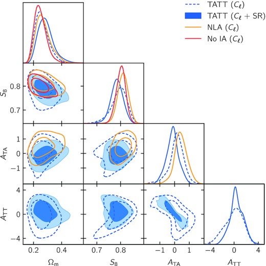
Constraints on cosmological and intrinsic alignment (IA) parameters from DES Y3 cosmic shear power spectra. The three colours refer to the assumed IA model: TATT in blue, NLA in orange, and no IA in red. The filled blue contours include information from shear ratios while the dashed ones do not. Shear ratios are not included for the NLA and no IA models.
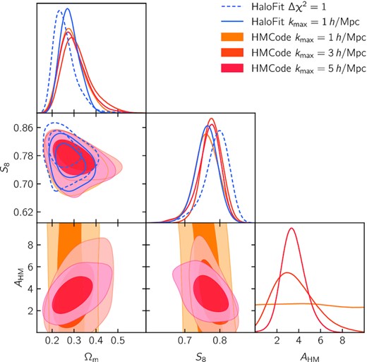
Constraints on cosmological and baryonic feedback parameters from DES Y3 cosmic shear power spectra. In blue, we show constraints for the fiducial model, i.e. using halofit. In orange to red, we show constraints using hmcode with one free parameter, while varying the kmax cut-off from 1 to |${5}\, {h}\, {\rm Mpc}^{-1}$| (see Fig. 4). We also show, with dashed lines, the constraints for the fiducial halofit model and the |$k_{\rm max}={1}\, h\, {\rm Mpc}^{-1}$| cut, which is even more conservative than our fiducial Δχ2 = 1 cut. Note that all constraints shown here use TATT to model intrinsic alignments and none include shear ratio information.
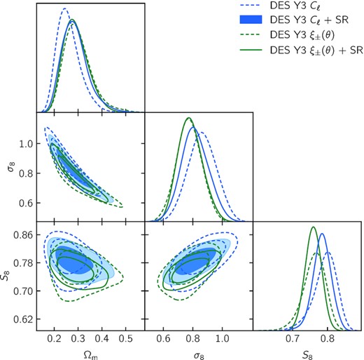
Comparison of cosmological constraints obtained from the analysis of cosmic shear two-point functions of DES Y3 data in real (in green, Amon et al. 2022; Secco et al. 2022) and harmonic space (in blue, this work). Solid contours indicate constraints that include shear ratio information Sánchez et al. (2021). We find ΔS8 = 0.025, with shear ratios, consistent with the expected statistical scatter σ(ΔS8) ∼ 0.02 predicted in Doux et al. (2021).
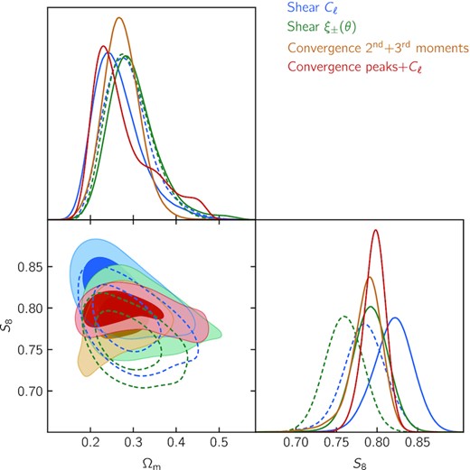
Comparison of cosmological constraints obtained from the analysis of DES Y3 lensing data using four different statistics: shear power spectra (this work, in blue), shear two-point functions (Amon et al. 2022; Secco et al. 2022, in green), convergence second and third order moments (Gatti et al. 2021b, in orange), and convergence peaks and power spectra (Zürcher et al. 2022, in red). For the first two, we have matched the modeling to that adopted for the analysis of non-Gaussian convergence statistics, namely restricting the intrinsic alignment model to NLA and fixing the total mass of neutrinos (see main text for a discussion of possible caveats). These constraints are shown by solid contours, whereas constraints obtained with the fiducial model are shown by the dashed contours, for reference. None of the constraints shown here include shear ratio information. Although the comparison requires some care, this figure highlights the overall consistency of DES Y3 lensing data and existing analyses.
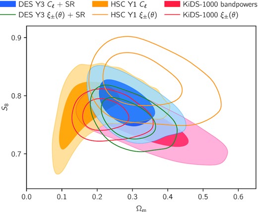
Comparison of cosmological constraints from the analysis of cosmic shear in harmonic (filled contours) and real space (contour lines) for DES Y3 (this work in blue, Amon et al. 2022; Secco, Samuroff et al. 2022 in green), HSC Y1 (Hikage et al. 2019; Hamana et al. 2020, 2022b, in yellow) and KiDS-1000 (Asgari et al. 2021, in red). We note that these results rely on different analysis and modelling choices.
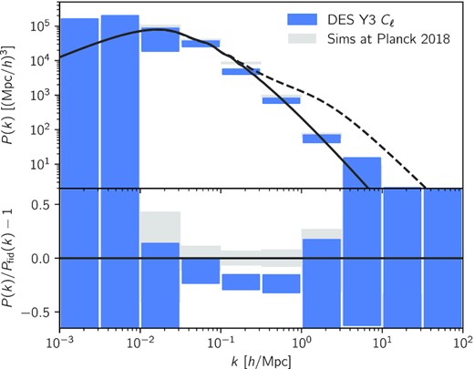
Matter power spectrum at redshift z = 0 reconstructed from DES Y3 shear power spectra, using a simplified version of the method of Tegmark & Zaldarriaga (2002). The fiducial linear matter power spectrum, computed at Planck 2018 cosmology (Planck Collaboration VI 2020), is shown by the solid, black line (the corresponding non-linear power spectrum is shown by the dashed, black line). The blue boxes, centred on |${(k, \hat{{\bf P}})}$| (see equation 33) and of height given by the square-root of the diagonal of the covariance matrix |$\bf{S}$| (see equation 34), show the reconstructed power spectrum within log-spaced k bins. In the background, we show in grey the result of the reconstruction for 1000 simulated data vectors drawn from the likelihood at Planckcosmology; however, in this case, the height of the boxes represents the standard deviation of the results, offering a simple check for the covariance matrix. The reconstructed power spectrum is about 20 per cent (or roughly 2σ) lower than the fiducial one around |$k\sim {0.3}\, h\, {\rm Mpc}^{-1}$|.
We also aim at constraining the effect of baryonic feedback using alternative scale cuts based on a kmax cut-off in Fourier space, as explained in Section 3.5.2. In order to validate the robustness of this alternative model, we follow a similar approach and consider predictions for the shear power spectra from four hydrodynamical simulations (Illustris, OWLS AGN, Horizon AGN, and MassiveBlack II), as shown in Fig. 5. We then build corresponding data vectors using halofit and a rescaling of the matter power spectrum, as in equation (25). Next, we analyse those data vectors using (i) the true model considered here (i.e.halofit and rescaling), and then (ii) hmcode with one free parameter. We finally test whether the (S8, Ωm) best-fitting parameters for the true model are within the 0.3σ contours of the posterior assuming hmcode.
When varying only AHM, we do find that this test passes for kmax = 1, 3, and 5 |$h\, {\rm Mpc}^{-1}$| with biases of 0.22σ at most (and typically 0.1σ), even though the inferred AHM parameter largely varies across simulations (we find posterior means of 2.2, 2.7, 3.4, and 3.6 for Illustris, OWLS AGN, Horizon AGN, and MassiveBlack II, respectively). This means that biases introduced by hmcode, if any, are not worse than potential projection effects found when using the true model, all of which are found to be below the level of 0.3σ. In addition, this also means that hmcode allows us to properly marginalize cosmological constraints over uncertainties in baryonic feedback.
4.4.2 Validation with Buzzard simulations
In this section, we use Buzzard simulations (see Section 4.1.3) to validate our measurement and analysis pipelines together. Precisely, we verify that (i) we are able to recover the true cosmology used when generating Buzzard simulations and (ii) the model yields a reasonable fit to the measured shear spectra.
We start by measuring cosmic shear power spectra and verify that the mean measurement (not shown) is consistent with the theoretical prediction from our fiducial model at the Buzzard cosmology, using the true Buzzard redshift distributions, and with a covariance recomputed with these inputs.
We then run our inference pipeline on the mean data vector, first with the covariance corresponding to a single realization, and then with a covariance rescaled by a factor of 1/16, to reflect the uncertainty on the average of the measurements. The first case is testing whether we can recover the true cosmology on average, while the second is a stringent test of the accuracy of the model, given that error bars are divided by |$\sqrt{16}=4$| with respect to observations with the DES Y3 statistical power. For these tests, the priors on shear and redshift biases are centered at zero, with a standard deviation of 0.005.
The 68 and 95 per cent confidence contours are shown in Fig. 9 for both covariances, using the fiducial χ2 < 1 scale cuts. We only show the contours for the best constrained parameters (Ωm, σ8, and S8) but we verified that the true cosmology is recovered in the full parameter space. We find that it is perfectly recovered in the first case and within 1σ contours in the second case, consistent with fluctuations on the mean Buzzard data vector. We find that the effective number of constrained parameters is Neff ≈ 7.8 in the first case, whereas, in the second case, we find Neff ≈ 9.6 (recall we fix the neutrino mass to zero for tests on Buzzard, so Nparam = 18 here). In the second test, we find that χ2 = 139.4 at the best-fitting parameters (maximum a posteriori) for N = 119 data points, and N − Neff degrees of freedom, such that the best-fitting χ2 corresponds to a probability-to-exceed of 2.7 per cent. For kmax cuts, we also recover the input cosmology within error bars and find χ2/(N − Neff) of 98.4/61.7, 191.6/146.1, and 254.5/217.8, respectively, for kmax of 1, 3, and 5 |$h\, {\rm Mpc}^{-1}$| (although note we will not use this combination of model and scale cuts on data). Together, these tests suggest that the accuracy of our fiducial model exceeds that required by the statistical power of DES Y3 data.
We then run our inference pipeline on each realization to visualize the scatter in the posteriors due to statistical fluctuations. This exercise allows us to verify that the model does not feature catastrophic degeneracies that have the potential to bias the marginal posterior distributions over cosmological parameters, in particular in the (S8, Ωm) plane. The contours are shown in Fig. 9, along with the contours obtained from the mean Buzzard data vector. We also compute the χ2 at best fit for each realization and find that the distribution is perfectly consistent with a χ2 distribution with N − Neff degrees of freedom, where we find Neff ≈ 7.8(2) in these cases.
5 BLINDING
We follow a blinding procedure, decided beforehand, that is meant to prevent confirmation and observer biases, as well as fine tuning of analysis choices based on cosmological information from the data itself. After performing sanity checks of our measurement and modelling pipelines that only drew from the data basic properties such as its footprint and noise properties, we proceeded to unblind our results in three successive stages as described below. It is worth noting, though, that as this work follows the real space analysis of Amon et al. (2022) and Secco et al. (2022), the blinding procedure is meant to validate the components of the analysis that are different, such as the cosmic shear power spectrum measurements, the scale cuts, and the covariance matrix.
Stage 1. The shape catalogue was blinded by a random rescaling of the measured conformal shears of galaxies, as detailed in Gatti et al. (2021c). This step preserves the statistical properties of systematic tests while shifting the inferred cosmology. A number of null tests were presented in Gatti et al. (2021c) to test for potential additive and multiplicative biases before deeming the catalogue as science-ready and unblinding it. In the Section 4.2, we repeated two of these tests in harmonic space, namely the test of the presence of B modes and the test of the contamination by the PSF.
Once all these tests had passed, we used the unblinded catalogue to measure the shape noise power spectrum and compute the Gaussian contribution to the covariance matrix. We then repeated the systematic and validation tests, in particular those based on Gaussian simulations where shape noise is inferred from the data.
Stage 2. Using the updated covariance matrix, we proceeded to validate analysis choices with synthetic data. We first determined fiducial scale cuts based on the requirement that baryonic feedback effects do not bias cosmology at a level greater than 0.3σ, as detailed in Section 3.5.1. We then verified that baryonic effects as predicted from a range of hydrodynamical simulations do not bias cosmology for alternative scale cuts, provided that hmcode(with a free baryonic amplitude parameter) is used instead of halofit, as detailed in Section 4.4.1. Finally, we verified that effects that are not accounted for in the model do not bias cosmology, e.g. PSF residual contamination in Appendix A, and higher order lensing effects and uncertainties in the matter power spectrum using the N-body Buzzard simulations in Section 4.4.2.
Stage 3. Before unblinding the data vector and cosmological constraints, we performed a last series of sanity checks. In particular, we verified that the model is a good fit to the data by asserting that the χ2 statistic at the best-fitting parameters corresponds to a probability-to-exceed above 1 per cent. We found that the best-fit χ2 is 129.3 for 119 data points and Neff ≈ 5.6 constrained parameters, corresponding to a probability-to-exceed of 14.6 per cent. We also verified that the marginal posteriors of nuisance parameters were consistent with their priors. Finally, we performed two sets of internal consistency tests, in parameter space and in data space. For the tests in parameter space, we compared, with blinded axes, constraints for (S8, Ωm) from the fiducial data vector with constraints from subsets of the data vector, first removing one redshift bin at a time, and then removing large or small angular scales, as detailed in items a and b of Appendix C1. The tests in data space, presented in Appendix C2, are based on the posterior predictive distribution (PPD), and follow the methodology presented in Doux et al. (2020). The PPD goodness-of-fit test yields a calibrated probability-to-exceed of 11.6 per cent. These tests are detailed in Appendix C, along with other post-unblinding internal consistency tests.
After this series of tests all passed, we plotted the data and compared it to the best-fitting model, as shown in Fig. 4, and finally unblinded the cosmological constraints, presented in the next section.
6 COSMOLOGICAL CONSTRAINTS
This section presents our main results. We use measurements of cosmic shear power spectra from DES Y3 data to constrain the ΛCDM model in Section 6.1. We then explore alternative analysis choices to constrain intrinsic alignments in Section 6.2 and baryonic feedback in Section 6.3. We compare our results to other weak lensing analyses of DES Y3 data in Section 6.4, namely the comic shear two-point functions (Amon et al. 2022; Secco et al. 2022), convergence peaks and power spectra (Zürcher et al. 2022) and convergence second- and third-order moments (Gatti et al. 2021b), and to weak lensing analyses from the KiDS and HSC collaborations in Section 6.5. Finally, as an illustrative exercise, we reconstruct the matter power spectrum from DES Y3 cosmic shear power spectra using the method of Tegmark & Zaldarriaga (2002) in Section 6.6. A number of internal consistency tests are also presented in Appendix C and the full posterior distribution is shown in Appendix D.
Note that, for all the constraints that are presented in the following sections, we have recomputed the effective number of constrained parameters and verified that the χ2 statistic at best fit corresponds to a probability-to-exceed above 1 per cent.
6.1 Constraints on ΛCDM
In comparison to constraints from Planck2018, we find a lower amplitude of structure S8. We estimate the tension with the parameter shift probability metric using the tensiometer package, which accounts for the non-Gaussianity of the posterior distributions (Raveri & Doux 2021), and find tensions of about 1.4σ and 1.5σ with and without shear ratios, respectively.
Finally, we note that DES Y3 shear data alone is not able to constrain the dark energy equation-of-state w. We find that the evidence ratio between wCDM and ΛCDM is Rw/Λ = 0.68(18), which is inconclusive, based on the Jeffreys scale. We thus find no evidence of a departure from ΛCDM, consistent with Amon et al. (2022) and Secco et al. (2022).
6.2 Constraints on intrinsic alignments
In this section, we focus on constraints on intrinsic alignments (IA) and explore the robustness of cosmological constraints with respect to the IA model.
In terms of model selection, we find that going from no IA to NLA, and then from NLA to TATT improves fits by Δχ2 = −0.3 and Δχ2 = −1.1, respectively, while introducing two and three more parameters. The evidence ratios are given by RNLA/TATT = 3.59(93), RnoIA/TATT = 17.5(43), and RnoIA/NLA = 4.88(11), marking a weak preference for NLA over TATT, but a substantial preference for no IA over TATT, according to the Jeffreys scale.
Cosmic shear analyses in harmonic space usually only exploit the E mode part of the power spectrum. However, as detailed in Section 3.2.3, tidal torquing generates a small B-mode signal, which may at least be constrained by our B-mode data. We validated our analysis pipeline by checking that (i) the E-to-B-mode leakage measured in our Gaussian simulations (see Section 4.1.1) is consistent with expectations from mixing matrices, (ii) we do recover correct IA parameters, with tighter constraints, for synthetic data vectors for different values of the IA parameters (including non-zero ATT). We obtain constraints that are consistent for cosmological parameters inferred without B-mode data. However, they seem to strongly prefer non-zero ATT, and are not consistent across redshift bins. This preference is indeed entirely supported by bin pairs 3,3 an 3,4, that have the highest χ2 with respect to no B mode, as shown in Fig. 8. Including B-mode data and freeing TATT parameters, the χ2 for those bins are reduced by 13.5 and 17.4, respectively, while all other bin pairs are unaffected (χ2 changed by less than 1). Indeed, we find that removing bin 3 entirely makes the preference for non-zero ATT disappear, with very small impact on the cosmology. We obtain very similar results when including shear ratios. We conclude from this experiment that DES Y3 data is not able to constrain the contribution of tidal torquing to the TATT model efficiently, leading to the model picking up potential flukes in the B-mode data, which has been verified to be globally consistent with no B modes. Future data will place stronger constraints on B modes and its potential cosmological sources.
6.3 Constraints on baryons
We now turn our attention towards baryonic feedback. Our fiducial analysis discards scales where baryonic feedback is expected to impact the shear power spectrum. However, we have shown in Section 4.4.1 that hmcode provides a model that is both accurate and flexible enough for our analysis, for scale cuts with kmax in the range 1–5 |$\, h\, {\rm Mpc}^{-1}$|.
When using hmcode with two free parameters, we find that the constraining power is entirely transferred to the second parameter, ηHM, with very little impact on cosmological constraints. For |${k_{\rm max}={5}\, {h}\, {\rm Mpc}^{-1}}$|, we find |${\eta _{\rm HM}=0.86^{+0.29}_{-0.35}}$| while AHM is unconstrained.
The previous constraints are based on our fiducial IA model, TATT. However, we showed in the previous section that the NLA model seems favoured by the data (using evidence ratios). If we use this model instead, as done in the KiDS-1000 analysis (Asgari et al. 2021), we find S8 = 0.790 ± 0.024 and |${A_{\rm HM}= 3.67^{+0.71}_{-0.92}}$|, although we note immediately that we have not validated our scale cuts against this specific model and that these results should be interpreted with caution.
Our results do not allow exclusion of the dark matter only value of AHM = 3.13 in either direction. In comparison to the hydrodynamical simulations we used in Section 3.2.4 to validate the model, constraints from data are closer to Massive Black II, although the uncertainty from shear power spectra alone is too large to discriminate between baryonic feedback prescriptions. Fig. 13 suggests that a better understanding of the effect of baryons on the distribution of matter will be an important task in order to be able to capture cosmological information at small scales. For the foreseeable future, this will likely require cross-correlating shear data with other probes that are sensitive to baryons, e.g. Compton-y maps of the thermal Sunyaev–Zeldovich (SZ) effect with CMB maps (see e.g. Pandey et al. 2021; Gatti et al. 2021a with DES Y3 data and Tröster et al. 2021 with KiDS-1000 data) or the kinetic SZ effect (Amodeo et al. 2021; Schaan et al. 2021). Another avenue is to exploit information from even smaller scales, e.g.using a principal component analysis to span a variety of scenarios from hydrodynamical simulations (see Huang et al. 2019 for the methodology and Huang et al. 2021 for an application to DES Y1 data) or a baryonification model (see Schneider & Teyssier 2015; Schneider et al. 2019, and Chen et al. 2022).
6.4 Consistency with other DES Y3 weak lensing analyses
In this section, we compare our results obtained from cosmic shear power spectra to other studies using DES Y3 lensing data, as detailed below. We first focus on the comparison with the real-space analysis of shear two-point functions presented in Amon et al. (2022) and Secco et al. (2022). The study presented here is its harmonic space counterpart, in the sense that we follow a very similar methodology and use the same fiducial model. We then extend the comparison to studies that incorporate non-Gaussian information from the DES Y3 convergence (mass) map (Jeffrey et al. 2021b), namely the analysis of peaks and power spectra from Zürcher et al. (2022), and the analysis of second and third-order moments from Gatti et al. (2021b). Figs 14 and 15 show cosmological constraints obtained from those studies, which are found to be in very good agreement, illustrating the internal consistency of DES Y3 shear analyses. See also Fig. 11 for a comparisom of all 1D marginal constraints.
6.4.1 Real space two-point functions ξ±.
Fig. 14 shows cosmological constraints obtained from two-point functions in real space (Amon et al. 2022; Secco et al. 2022) and in harmonic space (this work), both with and without including shear ratio information. We find that both studies yield very consistent cosmological constraints, with a preference for slightly higher S8 from shear power spectra. However, the difference between the means of the posteriors is ΔS8 = 0.031 when excluding shear ratios, which is fairly consistent with the expected statistical scatter σ(ΔS8) ∼ 0.02 predicted10 in Doux et al. (2021). In this preparatory study, we had shown on simulations that cuts on angular scales, which are inevitable in practice, induce a partial loss of information that differs for shear power spectra and two-point correlation functions. As a consequence, the posterior distributions of the two analyses are not expected to perfectly overlap. Considering that the observed difference ΔS8 is found to be on par with the expected scatter σ(ΔS8), we do not deem this difference to be significant.
The degeneracy directions are also found to be slightly different, with |$\alpha _{C_\ell }=0.595$| and |$\alpha _{\xi _\pm }=0.552$| for harmonic and real space analyses, respectively. When including shear ratios, the difference narrows down to ΔS8 = 0.025 and the best constrained direction is almost identical, with |$\alpha _{C_\ell }=0.598$| and |$\alpha _{\xi _\pm }=0.586$|. As a consequence of the higher value of S8 found here, the tension with Planckis reduced from 2.3σ in Amon et al. (2022) and Secco et al. (2022) to 1.5σ in this work.
For IA parameters, we find an overall excellent agreement (not shown). Although the real-space analysis shows a weak preference for negative ATA and positive ATT, we observe the same degeneracy between those parameters, with almost perfect overlap. The two parameters that describe redshift evolution are unconstrained in both cases, but the posteriors are also nearly identical. We also find that fixing the IA model to NLA results in a slightly higher value for S8.
6.4.2 Non-Gaussian statistics from mass maps.
Fig. 15 presents cosmological constraints from all four lensing analyses. Due to difficulties in modelling non-Gaussian statistics, both analyses of moments and peaks (Gatti et al. 2021b; Zürcher et al. 2022) include IA contributions using a model based on NLA, and both fix the total mass of neutrinos to the minimum value of 0.06 eV. In order to make the comparison more meaningful, we therefore re-analyse shear two-point functions and power spectra with these two changes, which tends to favour slightly higher values of S8 (either change individually also goes in this direction). We warn the reader that (i) despite matching important modeling choices, there remain differences in the analysis in terms of priors, modeling pipeline technology (e.g. Zürcher et al. 2022 uses an emulator) and methodology, and (ii) the scale cuts used for two-point functions were not validated for this specific model, and should be interpreted with caution. Nevertheless, this figure illustrates the high level of consistency of these analyses – all of which followed a similar blinding procedure – and of DES Y3 lensing data.
6.5 Comparison with other lensing surveys
In the past two years, both the HSC and KiDS collaborations have presented cosmic shear analyses of their data in harmonic and real space. Fig. 16 compares constraints obtained from DES Y3 data to those obtained from KiDS-1000 (Asgari et al. 2021) and HSC Y1 (Hikage et al. 2019; Hamana et al. 2020, 2022b). Uni-dimensional marginal distributions are also shown in Fig. 11. As shown in Doux et al. (2021) on simulations, statistical fluctuations are not expected to bias one estimator over the other and shift constraints in any specific direction, while unmodelled systematic effects might. We do not find any clear trend here.
Both KiDS-1000 and HSC analyses use NLA to model intrinsic alignments with fixed neutrino masses. However, we decide to present constraints that were obtained from the fiducial models assumed by each collaboration for simplicity. We also note that the KiDS-1000 analysis uses a ‘bandpowers’ estimator of shear power spectra that stems from an original measurement of two-point functions in real space with a thin spacing. A recent analysis (Loureiro et al. 2021) applying a pseudo-Cℓ estimator found very similar constraints on |$S_8 = 0.754^{+0.027}_{-0.029}$| between the bandpowers and pseudo-Cℓ estimators, despite appreciable differences in the intrinsic alignment parameter, likely due to how the two estimator cut large-scale information. Ignoring potential correlations due to overlapping survey areas, we find our results to be in agreement at the 0.7σ and 0.4σ levels with KiDS-1000 bandpowers and HSC Y1 Cℓ analyses. Finally, we find good agreement on the IA parameter ATA (not shown), although constraints remain broad for all three surveys.
6.6 Reconstruction of the matter power spectrum
In this section, we apply the method of Tegmark & Zaldarriaga (2002) to approximately reconstruct the linear matter power spectrum at present time, P(k), from DES Y3 shear power spectra. We immediately note that this exercise is strongly model dependent, in that it requires to assume a full cosmological model to relate shear power spectra to the matter power spectrum. Moreover, it presents subtleties in relating physical scales between the linear and non-linear power spectra, as discussed in Tegmark & Zaldarriaga (2002), and we will employ a simplified approach presented in the next paragraph. Nevertheless, assuming the Planck 2018 cosmology (Planck Collaboration VI 2020), we may compare the power spectrum reconstructed from DES Y3 data to the expectation from Planck, which is relevant in the context of the σ8 tension found in previous weak lensing surveys (Hikage et al. 2019; Hamana et al. 2020, 2022b; Asgari et al. 2021; Amon et al. 2022; Secco et al. 2022), and that we also observe in Fig. 10.
The result is shown in Fig. 17. The lower panel shows the reconstructed, binned ratio of the power spectrum with respect to the prediction from Planck 2018 (in blue), compared to the results obtained from simulated DES Y3 data vectors generated by sampling the likelihood at the Planck2018 cosmology (in grey). In the upper panel, we multiply these ratios by the fiducial linear power spectrum, shown in black. We find that the reconstructed spectrum is roughly 20 per cent lower than the prediction in the range |$k\sim {0.03}$|–1 |$\, h\, {\rm Mpc}^{-1}$| that is constrained by DES Y3 data. In particular, the reconstruction is about 2 σ low around |$k\sim {0.3}\, h\, {\rm Mpc}^{-1}$|, which remains close to the linear regime.
7 CONCLUSIONS
In this work, we have used data from the first three years of observations by the Dark Energy Survey (DES Y3), including a catalogue of over a hundred million galaxy shape measurements (Gatti et al. 2021c) split into four redshift bins (Myles et al. 2021), to measure tomographic cosmic shear power spectra. Our measurements over the DES Y3 footprint of 4143 deg2 are based on the pseudo-Cℓ method, with a consistent spherical sky approach using the namaster software (Alonso et al. 2019). We generally followed the DES Y3 methodology laid out in Amon et al. (2022), Secco et al. (2022) and the modelling choices presented in Krause et al. (2021) to infer cosmological constraints, and found |${S_8 \equiv \sigma _8 \sqrt{\Omega _{\rm m}/0.3} = 0.793^{+0.038}_{-0.025} \,\, (0.810)}$| using cosmic shear alone. We also included geometric information from small-scale galaxy–galaxy lensing ratios (Sánchez et al. 2021) to tighten the constraint to S8 = 0.784 ± 0.026 (0.798).
Following Amon et al. (2022) and Secco et al. (2022), we modeled intrinsic alignments with TATT (Blazek et al. 2019) that coherently includes tidal alignment (TA) and tidal torquing (TT) mechanisms. We found, as in Secco et al. (2022), that the data does not strongly favour this model over the simpler non-linear alignment (NLA) model, as the data does not seem to constrain the TT contribution efficiently (even when including B-modes in the analysis, which may be sourced by TT). In all cases, we find consistent cosmological constraints, although using NLA tightens constraints on S8 by about 25 per cent.
We include smaller scales that had been discarded in the fiducial analysis, switching from halofit to hmcode to model the non-linear matter power spectrum, thus including the effect of baryonic feedback, known to be a major source of uncertainty for cosmic shear at small scales (Chisari et al. 2018; Huang et al. 2019). We derived a set of scale cuts that approximately map to a cut-off kmax in Fourier modes. When raising kmax from 1 to |${5}\, {h}\, {\rm Mpc}^{-1}$|, we found consistent cosmological constraints, while the extra statistical power appears to mainly constrain the baryonic feedback parameter, |${A_{\rm HM}= 3.52^{+0.94}_{-1.2} \,\, (1.620)}$|. This result does not rule out the dark matter-only case (AHM = 3.13) nor the predictions from the hydrodynamical simulations we considered in this work. Given current error bars and theoretical uncertainties, it therefore remains difficult to extract small-scale cosmological information that is present in our cosmic shear data, thus highlighting the need to better understand the effect of baryonic processes on the clustering of matter, especially for future surveys (see e.g. Martinelli et al. 2021).
This analysis complements other weak lensing analyses of DES Y3 data, namely the analysis of cosmic shear two-point correlation functions presented in Amon et al. (2022) and Secco et al. (2022), convergence second- and third-order moments (Gatti et al. 2021b), and convergence peaks and power spectra (Zürcher et al. 2022), the latter two being based on maps from Jeffrey et al. (2021b). With respect to the real-space two-point functions, we find very similar constraints, with a value of S8 slightly higher by ΔS8 = 0.025 when including shear ratios, perfectly consistent with statistical fluctuations of order σ(ΔS8) ∼ 0.02 predicted in Doux et al. (2021). The comparison of constraints from Gaussian and non-Gaussian statistics delivers an overall coherent picture, highlighting the cosmological information beyond two-point measurements and pointing towards the modeling improvements required for future analyses. This analysis thus provides an important consistency check of DES Y3 lensing data. It also demonstrates the feasibility of conducting a harmonic space analysis over a wide survey footprint, which could be combined with other estimators, such as the real-space correlation functions, into a joint analysis in the future. To do so, one would need to compute an accurate estimate of the cross-covariance of the different statistics considered, or to perform a simulation-based, likelihood-free analysis (see e.g.Jeffrey et al. 2021a).
At last, we compared our results to those obtained by other weak lensing studies from the Hyper Suprime-Cam and Kilo-Degree Survey collaborations and found consistent constraints on cosmology. We also compared our results to constraints from observations of the cosmic microwave background. We found that the tension with Planck 2018 in S8, computed with the parameter shift probability (Raveri et al. 2020; Raveri & Doux 2021), is 1.5σ in this work, whereas it is 2.3σ in Amon et al. (2022) and Secco et al. (2022). This shift is reflected in the inferred linear matter power spectrum, in excess by about 20 per cent in the range |$k\sim 3\times 10^{-2}\, h\, {\rm Mpc}^{-1}$| to |$1\, h\, {\rm Mpc}^{-1}$| for Planckwith respect to DES Y3. Future observations, such as the complete data from the six-year program of the DES and data from the next generation of surveys including LSST, Euclid and Roman, as well as methodological improvements will be necessary to determine whether this apparent tension is the sign of an incorrect treatment of systematic effects, or of new physics.
ACKNOWLEDGEMENTS
The authors would like to thank Masahiro Takada for useful discussions that motivated this work, and David Alonso and Andrina Nicola for discussions about the pseudo-Cℓ method.
This research has made use of NASA’s Astrophysics Data System, adstex (https://github.com/yymao/adstex), numpy (Harris et al. 2020), scipy (Virtanen et al. 2020), matplotlib (Hunter 2007), numba (Lam et al. 2021), astropy (Astropy Collaboration 2013, 2018), healpy (Zonca et al. 2019), namaster(Alonso et al. 2019), cosmosis software (Zuntz et al. 2015), cosmolike (Eifler et al. 2014; Krause & Eifler 2017), getdist (Lewis 2019), and polychord (Handley et al. 2015).
Funding for the DES Projects has been provided by the U.S. Department of Energy, the U.S. National Science Foundation, the Ministry of Science and Education of Spain, the Science and Technology Facilities Council of the United Kingdom, the Higher Education Funding Council for England, the National Center for Supercomputing Applications at the University of Illinois at Urbana-Champaign, the Kavli Institute of Cosmological Physics at the University of Chicago, the Center for Cosmology and Astro-Particle Physics at the Ohio State University, the Mitchell Institute for Fundamental Physics and Astronomy at Texas A&M University, Financiadora de Estudos e Projetos, Fundação Carlos Chagas Filho de Amparo à Pesquisa do Estado do Rio de Janeiro, Conselho Nacional de Desenvolvimento Científico e Tecnológico and the Ministério da Ciência, Tecnologia e Inovação, the Deutsche Forschungsgemeinschaft and the Collaborating Institutions in the Dark Energy Survey.
The Collaborating Institutions are Argonne National Laboratory, the University of California at Santa Cruz, the University of Cambridge, Centro de Investigaciones Energéticas, Medioambientales y Tecnológicas-Madrid, the University of Chicago, University College London, the DES-Brazil Consortium, the University of Edinburgh, the Eidgenössische Technische Hochschule (ETH) Zürich, Fermi National Accelerator Laboratory, the University of Illinois at Urbana-Champaign, the Institut de Ciències de l’Espai (IEEC/CSIC), the Institut de Física d’Altes Energies, Lawrence Berkeley National Laboratory, the Ludwig-Maximilians Universität München and the associated Excellence Cluster Universe, the University of Michigan, NSF’s NOIRLab, the University of Nottingham, The Ohio State University, the University of Pennsylvania, the University of Portsmouth, SLAC National Accelerator Laboratory, Stanford University, the University of Sussex, Texas A&M University, and the OzDES Membership Consortium.
Based in part on observations at Cerro Tololo Inter-American Observatory at NSF’s NOIRLab (NOIRLab Prop. ID 2012B-0001; PI: J. Frieman), which is managed by the Association of Universities for Research in Astronomy (AURA) under a cooperative agreement with the National Science Foundation.
The DES data management system is supported by the National Science Foundation under Grant Numbers AST-1138766 and AST-1536171. The DES participants from Spanish institutions are partially supported by MICINN under grants ESP2017-89838, PGC2018-094773, PGC2018-102021, SEV-2016-0588, SEV-2016-0597, and MDM-2015-0509, some of which include ERDF funds from the European Union. IFAE is partially funded by the CERCA program of the Generalitat de Catalunya. Research leading to these results has received funding from the European Research Council under the European Union’s Seventh Framework Program (FP7/2007-2013) including ERC grant agreements 240672, 291329, and 306478. We acknowledge support from the Brazilian Instituto Nacional de Ciência e Tecnologia (INCT) do e-Universo (CNPq grant 465376/2014-2).
This manuscript has been authored by Fermi Research Alliance, LLC under Contract No. DE-AC02-07CH11359 with the U.S. Department of Energy, Office of Science, Office of High Energy Physics.
DATA AVAILABILITY
A general description of DES data releases is available on the survey website at https://www.darkenergysurvey.org/the-des-project/data-access/. DES Y3 cosmological data has been partially released on the DES Data Management website hosted by the National Center for Supercomputing Applications at https://des.ncsa.illinois.edu/releases/y3a2. This includes Gold products, PSF modelling, Balrog catalogues, Deep Fields data and the Y3 galaxy catalogs, including the redshift distributions used in this analysis. The cosmosis software (Zuntz et al. 2015) is available at https://bitbucket.org/joezuntz/cosmosis/wiki/Home. The measurement code, used in this analysis to interface DES catalogues and namaster, can be obtained upon request to the corresponding author.
Footnotes
Note that since power spectra for different redshift bin pairs are correlated, the requirement that each pair ab verifies |$\Delta \chi ^2_{ab}\lt 0.1$| yields a global Δχ2 ≈ 0.34.
Note that this prediction depends strongly on the two sets of scale cuts and the survey configuration.
REFERENCES
APPENDIX A: POINT SPREAD FUNCTION
This section presents the results of our tests for potential contamination of shear power spectra from the point spread function (PSF) and complements those presented in Jarvis et al. (2021) and Gatti et al. (2021c).
We specifically focus on the additive biases due to PSF misestimation using ρ-statistics (Rowe 2010) following the same diagnostics as Gatti et al. (2021c). We expect other contributions like the brighter-fatter effect, dependencies of the PSF model residuals on star and galaxy colours, and tangential shear around stars to be negligible, as discussed in section 5 of Gatti et al. (2021c).
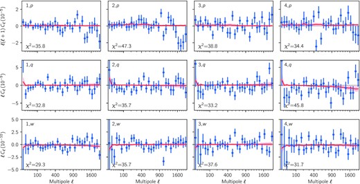
Cross-power spectra between galaxy shapes in the four redshift bins (from left to right) with PSF parameters |$\boldsymbol {p}$|, |$\boldsymbol {q}$|, and |$\boldsymbol {w}$| (from top to bottom). The measurements are shown in blue, with error bars computed from 18 000 Gaussian simulations using the DES Y3 catalogue ellipticities and positions, as explained in Section 4.1.1. The model from equations (A3) to (A5) at best fit is shown by the red line, while the band shows the uncertainty. We find χ2 statistics with respect to the best fit between 29.3 and 45.8 (29.3–47.3 for the null hypothesis) for 32 degrees of freedom, shown in the lower left corner for each panel, corresponding to a minimum probability-to-exceed of 0.04.
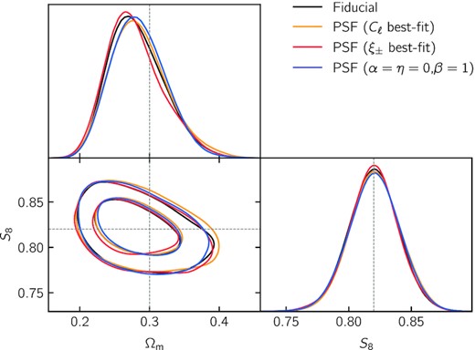
Impact of PSF contamination of the measured shear spectra on cosmological constraints. Fixing the values of the PSF model parameters (α, β, and η) at the best-fitting values inferred from power spectra (blue contours) or two-point functions (red), and at the expected values (orange), we contaminate a noiseless data vector using the model in equation (A2) and compare cosmological constraints to those obtained from the noiseless data vector (black).
We first measured the cross power spectra of the shear and the PSF parameters |$\boldsymbol {p}$|, |$\boldsymbol {q}$|, and |$\boldsymbol {w}$|. We then repeated these measurements using 18 000 Gaussian simulations, as described in Section 4.1.1, to obtain their covariance matrix. To calculate the cross power spectra between the PSF parameters [right-hand side of equations (A3)–(A5)], we split the catalog into two halves that we cross-correlate, which effectively cancels out the shot noise. We then find the best-fitting scalar parameters α, β, η over all scales and three cross-spectra types for each tomographic redshift bin using Markov chain Monte Carlo (MCMC) samples generated with the public software package emcee (Foreman-Mackey et al. 2013). This approach is adapted from the measurements performed in the real space analysis (Amon et al. 2022) using the same tomographic split, and the non-tomographic measurement from Jarvis et al. (2021).
We present the best fit α, β, η values in Table A1. While α is consistent with the expected value of 0 and with real space results from Amon et al. (2022), β and η values are different. We associate the difference to the fact that the real space analysis uses much smaller scales, down to the sub-arcminute range, while our harmonic space analysis only captures features larger than a few arcminutes. The total goodness of fit on the stacked data vector of the shear and PSF cross-spectra χ2 for 93 degrees of freedom varies between 99.5 and 117.3 across redshift bins. As in the real space analysis, the χ2 values are rather large for all but the lowest redshift bin, with the probability-to-exceed being 0.045. Subsequently in Fig. A1, we show the best-fitting model to the cross power spectra for each redshift bin and report the χ2 values for each shear and PSF parameter cross-spectrum separately.
| Bin 1 | Bin 2 | Bin 3 | Bin 4 | |
|---|---|---|---|---|
| α | |$0.003_{-0.007}^{+0.007}$| | |$0.014_{-0.008}^{+0.008}$| | |$0.008_{-0.010}^{+0.010}$| | |$0.012_{-0.011}^{+0.011}$| |
| β | |$0.02_{-0.36}^{+0.36}$| | |$-0.07_{-0.38}^{+0.38}$| | |$0.16_{-0.38}^{+0.39}$| | |$-0.74_{-0.47}^{+0.46}$| |
| η | |$-5.4_{-4.4}^{+4.3}$| | |$0.4_{-4.8}^{+4.8}$| | |$1.6_{-5.0}^{+5.1}$| | |$-5.4_{-5.8}^{+5.9}$| |
| χ2 | 99.5 | 116.3 | 113.4 | 117.3 |
Finally, we propagate the PSF bias in equation (A1) to compute the expected contamination of the shear power spectra using the model of equation (A2), in order to test its impact on cosmology. We do so using the best-fitting values for the α, β, and η parameters from our analysis in harmonic space, the best fit from the real space analysis in Amon et al. (2022) and the expected values α = η = 0 and β = 1, consistent with non-tomographic results from Jarvis et al. (2021). Fig. A2 shows that the impact on cosmological constraints is negligible.
APPENDIX B: VALIDATION ON SYNTHETIC DATA
This section illustrates the validation of the modelling pipeline on synthetic data, as described in Section 4.4.1. Fig. B1 shows the impact of the choice for the non-linear matter power spectrum, whereas Fig. B2 validates the use of hmcode to probe the small-scale portion of our measurements, based on its robustness to various baryonic feedback prescriptions from four different hydrodynamical simulations.
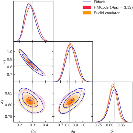
Test of the impact of the non-linear matter power spectrum on cosmological constraints. We analyse three synthetic data vectors with the fiducial model using halofit and fiducial scale cuts. Constraints obtained from the fiducial data vector are shown in blue, with the mean of the posterior shown by the blue cross. These constraints are compared to those obtained from data vectors computed with hmcode(red, AHM = 3.13) and the Euclid Emulator (orange). The innermost 0.3 σ contours (underlined in dashed lines) encompass the mean of the fiducial posterior.
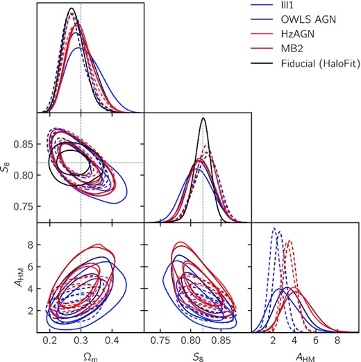
Validation of the baryonic feedback modelling with hmcode. The four coloured posteriors are obtained from shear power spectra that include the effect of baryons as predicted by four hydrodynamical simulations (see Fig. 5). Solid (dashed) lines were obtained using the scale cuts at |$k_{\rm max}={3}\, h\, {\rm Mpc}^{-1}$| (|$k_{\rm max}={5}\, {h}\, {\rm Mpc}^{-1}$|). Despite preferring very different values of AHM (the dark matter-only case corresponds to AHM = 3.13), the cosmology is recovered in all cases. For comparison, the black contours show the posterior obtained from the fiducial data vector analysed with halofit with the scale cuts at |$k_{\rm max}={3}\, h\, {\rm Mpc}^{-1}$|.
APPENDIX C: INTERNAL CONSISTENCY
This section presents a number of tests in parameter (Appendix C1) and data space (Appendix C2) for the fiducial run, i.e. using our fiducial ΛCDM model and scale cuts, and excluding shear ratio information.
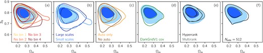
Robustness tests of cosmological constraints, comparing variations in analysis choices to the fiducial constraints in blue. We first repeat the analysis removing part of the data vector, according to (a) redshift bins, (b) scales, and (c) auto-power spectra. We then modify certain parts of the analysis, namely (d) the covariance matrix, (e) the methodology to marginalize over uncertainties in the redshift distributions, and (f) the measurement resolution. See Appendix C1 for details.
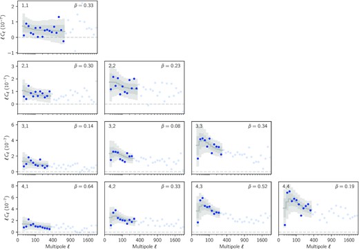
Goodness of fit test for the fiducial run using the posterior predictive distribution (PPD) methodology of Doux et al. (2020). The data are shown by the blue circles, which are filled for data points within fiducial scale cuts. The grey line shows the mean of the PPD realizations, whereas the grey bands show the 1σ and 2σ percentiles of the PPD. The calibrated p-value for each panel is shown in the upper right corner.
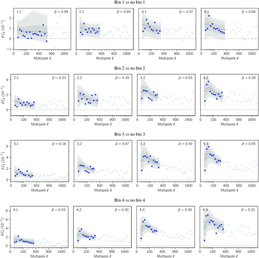
Internal consistency of the four redshift bins (removing one at a time) with the PPD in grey and data in blue. See Fig. C2 for details.
C1 Robustness of cosmological constraints
We first perform a series of tests, listed below, to assert the robustness of cosmological constraints presented in Section 6.1. Fig. 11 presents uni-dimensional marginal distributions for these tests in sections (d) and (e). We also show the 2D marginal distributions in the (S8, Ωm) plane in Fig. C1, in the following order:
Redshift test. Many parts of the cosmological model (including intrinsic alignments) are redshift dependent by construction, whereas systematic effects may differentially impact the four redshift bins. To test the robustness of the cosmological constraints to such effects, we therefore perform the analysis of cosmic shear power spectra removing one bin at a time (e.g. when removing bin 2, we remove the bin pairs 2,1, 2,2, 3,2 and 4,2 from the data vector), and show contours in Fig. C1, panel (a). While contours widen, as expected, and some degeneracies with ATA appear to create some tails in the posteriors, we find an overall excellent agreement, with no visible trend.
Large versussmall scales. As discussed throughout the paper, the non-linear scales play a crucial role in this analysis, as they contain a significant amount of cosmological information, but are also the most difficult to model. Using our fiducial set of scale cuts, we split the data vector between large and small scales as follows: for each redshift bin pair, we find the multipole ℓthr, within the scale cuts ℓmin ≤ ℓ ≤ ℓmax, that results in approximately equal signal-to-noise ratio S/N on both sides, i.e.|${S/N_{\ell _{\rm min}\le \ell \le \ell _{\rm thr}} \approx S/N_{\ell _{\rm thr}\le \ell \le \ell _{\rm max}}}$|. This procedure leaves us with 58 and 61 data points for large and small scales, respectively. We find that constraints using either only large scales or only small scales are very similar in width and in very good agreement with each other. The broadening of the posteriors seems related to partial degeneracies with intrinsic alignment parameters, in particular ATT. Nevertheless, they are in very good agreement with the constraints from the full analysis.
Autopower spectra. The pseudo-Cℓ estimator we use here requires the subtraction of the noise power spectrum, which is estimated analytically from the shape catalogue here, following Nicola et al. (2021). In order to evaluate the potential impact of a misestimation, we analyse our data without autopower spectra, i.e. removing bin pairs 1,1, 2,2, 3,3, and 4,4 from the data vector (no auto), and then using only those pairs (auto only). We find constraints that are wider but consistent with the full analysis, with no clear indication for an issue with noise spectrum subtraction.
Covariance. As described in Section 3.3, our covariance matrix is a hybrid matrix that uses namaster to evaluate the Gaussian contribution with the effects of the mask and binning properly accounted for, and cosmolike to evaluate the non-Gaussian contribution, at the fiducial Planck 2018 cosmology. We have also used darkgridV1 simulations (Zürcher et al. 2022) to obtain an empirical estimate of the covariance matrix, for comparison and validation of our analytical (and therefore noiseless) estimate. We test the impact of this choice by using the empirical covariance in our cosmological analysis, and find that our constraints are almost insensitive to this choice, showing the excellent agreement of the two covariance matrices.
hyperrank. Throughout this work, we have employed the fiducial approach over marginalizing over redshift distribution biases, Δza’s, in order to account for uncertainty in the redshift distributions. However, the DES Y3 redshift pipeline produced samples of the redshift distributions that can be properly marginalized over using either the multirank or HyperRank methods, by sampling, respectively, realizations themselves, or a set of hyperparameters used to rank and select realizations (for details, see Cordero et al. 2022). We do so here and find cosmological constraints in excellent agreement with the fiducial analysis, with roughly 15 per cent smaller uncertainty on S8 for both techniques.
Resolution. As detailed in Section 3.1, the pseudo-Cℓ estimator is based on pixelized healpix maps of the shear catalogue. However, as discussed in Nicola et al. (2021), the effects of the pixelization of the shear field depend both on the density of galaxies and the chosen resolution. We used a resolution parameter of Nside = 1024, which allows us to probe multipoles up to ℓ ∼ 2000, while yielding a relatively complete mask, without too many empty pixels in the survey area, and with a mean number of galaxies per pixel of around 17.2–17.5 for all four bins. This means that we are in the regime where the shear maps are that of the averaged shear field (as opposed to the sampled shear field) and that we may use standard healpix window functions to correct for the smoothing that has taken place. In order to verify the impact on cosmological constraints, we repeat the measurements, including noise power spectrum and Gaussian covariance estimation, at Nside = 512. We do observe expected differences in the shear power spectra – almost negligible at large scales and growing up to about the size of the error bars at ℓ ∼ 1024, with no clear trend – but find negligible impact on cosmology.
C2 Internal consistency of data with posterior predictive distributions
We apply the methodology developed of Doux et al. (2020) based on the posterior predictive distribution (PPD) to test the internal consistency of our data. In a nutshell, the method uses a parameter posterior sample and compares simulated realizations of the data vector drawn from the likelihood at these parameter values to the observed data vector. The test is subsequently calibrated using simulated data vectors, to correct for posterior volume effects, as detailed in Doux et al. (2020).
We first perform a goodness-of-fit test, where the posterior sample comes from the fiducial run, and simulated realizations are independent of the observed data, and find a calibrated p-value of 11.6 per cent. The PPD samples are shown in grey in Fig. C2 along with the observed data in blue.
We then perform consistency tests of the type A versus B, i.e.where we divide the data in two disjoint parts A and B, use B to obtain a posterior sample, and generate from those samples realizations of A to be compared to the real data, in a way that accounts for the correlation between A and B. Specifically, we split the data according to redshift bins and scales, using the same splits as in item a and item b of the previous section. We illustrate the redshift consistency test in Fig. C3 and summarize the results in Table C1, finding no indication of inconsistency.
| Test | Calibrated p-value |
|---|---|
| Goodness of fit | 0.116 |
| Bin 1 versusno bin 1 | 0.998 |
| Bin 2 versusno bin 2 | 0.020 |
| Bin 3 versusno bin 3 | 0.080 |
| Bin 4 versusno bin 4 | 0.876 |
| Small versuslarge scales | 0.395 |
| Large versussmall scales | 0.212 |
| Test | Calibrated p-value |
|---|---|
| Goodness of fit | 0.116 |
| Bin 1 versusno bin 1 | 0.998 |
| Bin 2 versusno bin 2 | 0.020 |
| Bin 3 versusno bin 3 | 0.080 |
| Bin 4 versusno bin 4 | 0.876 |
| Small versuslarge scales | 0.395 |
| Large versussmall scales | 0.212 |
| Test | Calibrated p-value |
|---|---|
| Goodness of fit | 0.116 |
| Bin 1 versusno bin 1 | 0.998 |
| Bin 2 versusno bin 2 | 0.020 |
| Bin 3 versusno bin 3 | 0.080 |
| Bin 4 versusno bin 4 | 0.876 |
| Small versuslarge scales | 0.395 |
| Large versussmall scales | 0.212 |
| Test | Calibrated p-value |
|---|---|
| Goodness of fit | 0.116 |
| Bin 1 versusno bin 1 | 0.998 |
| Bin 2 versusno bin 2 | 0.020 |
| Bin 3 versusno bin 3 | 0.080 |
| Bin 4 versusno bin 4 | 0.876 |
| Small versuslarge scales | 0.395 |
| Large versussmall scales | 0.212 |
APPENDIX D: FULL POSTERIOR DISTRIBUTION
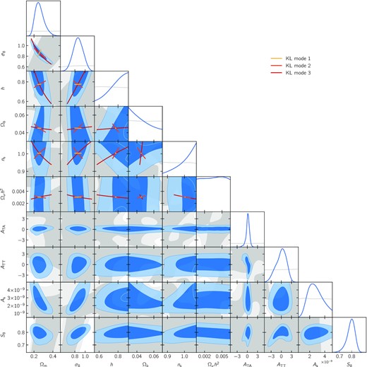
Posterior (in blue) and prior (in grey) distributions for the fiducial ΛCDM constraints from DES Y3 shear power spectra (without shear ratios) presented in Section 6.1, showing cosmological and intrinsic alignment parameters (note that the ranges are adjusted to the posterior for readability). Although we sample over As with a flat prior, we apply the KL decomposition (Raveri & Hu 2019; Raveri et al. 2020; Raveri & Doux 2021) in the space of log Ωm, log σ8, log h, log Ωb, log ns, and log Ωνh2. The best constrained directions in this parameter space, corresponding to the first three modes of the KL decomposition, are represented in yellow, orange, and red.
