


ABSTRACT
The Square Kilometre Array (SKA) is the largest radio interferometer under construction in the world. The high accuracy, wide-field, and large size imaging significantly challenge the construction of the Science Data Processor (SDP) of SKA. We propose a hybrid imaging method based on improved W-Stacking and snapshots. The w-range is reduced by fitting the snapshot uv plane, thus effectively enhancing the performance of the improved W-Stacking algorithm. We present a detailed implementation of WS-Snapshot. With full-scale SKA1-LOW simulations, we present the imaging performance and imaging quality results for different parameter cases. The results show that the WS-Snapshot method enables more efficient distributed processing and significantly reduces the computational time overhead within an acceptable accuracy range, which would be crucial for subsequent SKA science studies.
1 INTRODUCTION
Existing wide-field imaging algorithms are dedicated to correcting the phase errors introduced by the w-term. Crane & Napier (1989) first introduced the 3D-FFT algorithm to direct imaging, but this algorithm requires significant computational resources. The polyhedron imaging method, or image-plane faceting, was introduced to decrease computational costs. It is a more cost-effective alternative to the 3D-FFT, which has been used for wide-field imaging (Crane & Napier 1989). A variation of this approach, using coplanar rather than polyhedral facets, was proposed by Kogan & Greisen (2009).
As discussed in Cornwell et al. (2012), Ord et al. (2010), Cornwell & Perley (1992), Brouw (1971), and Bracewell (1984), the sampled points in V(u, v, w) space can be considered to be in the same plane for snapshot observations.
The W-Projection algorithm projects V(u, v, w) to the plane with w = 0, followed by a 2D-FFT to do the visibility function-to-image conversion (Cornwell, Golap & Bhatnagar 2003, 2008). Cornwell et al. (2012) further presented a novel algorithm to correct w in combination with W-Projection and snapshots, which is called the W-Snapshot algorithm.
In addition to W-Projection, W-Stacking has been proposed to correct for the w-term, the main idea of which is to discretize w in V(u, v, w) space and finally to weight the results of each w-plane cumulatively (Humphreys & Cornwell 2011; Offringa et al. 2014).
Recent work has effectively combined the methods discussed above. In particular, the DDFacet imager (Tasse et al. 2018) combines the facet-based approach with W-projection. It employs coplanar facets, and uses a per-facet version of a modified W-kernel to image each facet using W-projection. Recent versions of the WSClean imager (Offringa et al. 2014) also implement facet-based imaging, but rather using W-Stacking. This has complex computational trade-offs: the use of physically smaller (than the image) facets allows for smaller W-kernels or fewer W-Stacks, which offsets the computational cost of imaging a large number of facets (which in itself is an embarrassingly parallel problem, allowing for very efficient parallel implementations). Both packages support on-the-fly baseline-dependent averaging (BDA), which further reduces comptational load. In the case of DDFacet, the BDA is done on a per-facet basis, thus allowing for very aggressive averaging factors. The facet approach also naturally lends itself to application of direction-dependent effects (DDEs) on a per-facet basis. Alternatively, the AW-projection technique proposed by Bhatnagar et al. (2008) combines W-projection with per-baseline gridding kernels, which also serves to correct DDEs. A full comparison of these approaches, as well as treatment of DDEs, is outside the scope of this paper. They do, however, signpost the way to how different imaging approaches may be combined.
Based on the IW-Stacking algorithm, Arras et al. (2021) implemented efficient and accurate gridding and degridding operators, i.e. Ducc.wgridder.1 The Ducc.wgridder can solve the w-term effect with high accuracy (down to ≈10−12) and performs well in terms of computation time and memory consumption in practice. Ducc.wgridder is written in C++ and supports multiple threads to improve performance. Due to its outstanding processing performance and accuracy, Ducc.wgridder quickly became a vital software package and has been widely used in radio interferometer imaging.
However, in the case of large FOVs and large image sizes, e.g. the 10 square deg of FOV in continuum imaging of SKA1-Low and the image size of 215 pixels (Cornwell et al. 2012; Scaife 2020), we noticed deficiencies while using IW-Stacking (Ducc.wgridder) for wide-field imaging. We tested the performance with a range of threads from 1 to 40 and different scales such as 4 K (4096 × 4096), 8 K (8192 × 8192), and 16 K (16 384 × 16 384), respectively.
The test results are shown in Fig. 1. When imaging calculation is performed on large images, there is no longer any way to increase the final processing speed by increasing the number of threads, which is a limitation of IW-Stacking for SKA large-scale data processing.
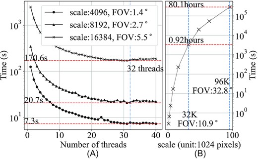
(A): The diagram of time consumption of IW-Stacking (Ducc.wgridder) with different number of threads. (B): The diagram of time consumption of IW-Stacking (Ducc.wgridder) in different image scales running at a 32-core server.
To meet the requirements of large-scale imaging, it is worth improving processing performance as much as possible while ensuring sufficient imaging accuracy. Reducing the number of w-planes is a possible method to reduce the calculation time. Snapshot imaging allows a significant reduction of w-range by coordinate transformation based on splitting visibility data into multiple snapshot observations (Brouw 1971; Bracewell 1984; Ord et al. 2010; Cornwell et al. 2012). To fully take advantage of the excellent performance of 'improved W-Stacking’, we propose a hybrid algorithm WS-Snapshot that has the advantages of both 'improved W-Stacking’ and snapshot algorithms.
We introduce the WS-Snapshot algorithm in Section 2, investigate its imaging accuracy and performance through practical tests in Section 3, and discuss some limitations of WS-Snapshot in Section 4.
2 DISTRIBUTED WS-SNAPSHOT ALGORITHM
2.1 WS-Snapshot
WS-Snapshot extends W-Snapshot by using IW-Stacking to correct Δw instead of W-Projection. We first obtain the current best plane in u,v,w space by least-squares fit. We then use IW-Stacking to correct Δw based on the fitted plane and perform snapshot imaging. We finally reproject the results of each snapshot from a distorted coordinate system to a normal coordinate system. Two parameters, a and b (equation 3), can be stored as the projection parameters of the image obtained by the snapshot observation, which in the current Flexible Image Transport System (FITS) are PV2_1 and PV2_2, respectively (Ord et al. 2010).
The computational complexities of W-Snapshot, W-Stacking, and WS-Snapshot are shown in Table 1. Although WS-Snapshot has NxNy more reprojection operations than W-Stacking for a single snapshot imaging, the w-range is significantly reduced after w-plane fitting. Take the example given in Fig. 2. The w-range is reduced from 45 511 m to 239 m after plane fitting, making the computational overhead required for the final WS-Snapshot to complete snapshot imaging comparable to W-Stacking or even smaller. As the FOV and image scale increase, the time consumed by both WS-Snapshot and W-Stacking increases accordingly. However, the time increase of WS-snapshot is much lower than that of W-Stacking. For reference, we also include the notional computational complexity of the DDFacet approach. Note that the number of facets Nfac can be taken to be roughly equivalent to the FOV squared. These figures should be taken with a serious caveat, as the scaling constants can be very different. In particular, the aggressive BDA strategy employed by DDFacet (see above) can easily yield compression factors of B ≫ 10 for small facets (large Nfac), but this is a complicated scaling relationship. It is also essential to clarify that WS-Snapshot is a time-slice-oriented data processing method, while DDFacet parallelizes over facets.
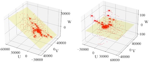
The diagram of uvw distribution in a snapshot. The left and right diagrams show the w-plane before (w-range = 45,511 m) and after (w-range = 239 m) plane fit, respectively.
Computational Complexity. Nx and Ny are the pixel size of the image in height and width, respectively, FOV is the field of view, Wrange and |$W_{\rm range\_fit}$| are the values of w-range before and after the w-plane fitting, respectively. Nvis is the amount of visibility data. Nfac is the number of facets. B is the BDA compression factor. The computational cost for FFTs and gridding is shown separately.
| Method | FFT cost | Gridding cost |
|---|---|---|
| W-Snapshot(snapshot imaging) | |$\mathcal {O}(N_{x}N_{y}\log ({N_{x}N_{y}}))$| | |$\mathcal {O}(N_{\rm vis}$|) |
| W-Stacking | |$\mathcal {O}(W_{\rm range} \times FOV \times N_{x}N_{y}\log ({N_{x}N_{y}})$|) | |$\mathcal {O}(N_{\rm vis})$| |
| WS-Snapshot(snapshot imaging) | |$\mathcal {O}(W_{\rm range\_fit} \times FOV \times N_{x}N_{y}\log ({N_{x}N_{y}}) + N_{x}N_{y}$|) | |$\mathcal {O}(N_{\rm vis}$|) |
| DDFacet | |$\mathcal {O}(N_{x}N_{y}\log ({N_{x}N_{y}/N_{\rm fac}) + N_{x}N_{y}}$|) | |$\mathcal {O}(N_{\rm vis}N_{\rm fac}/B)$| |
2.2 Algorithm implementation
We implement a WS-Snapshot function based on the Radio Astronomy Simulation, Calibration, and Imaging Library (RASCIL2). RASCIL is a crucial software package for SKA simulation and parallel data processing. RASCIL integrates with Ducc.wgridder to improve the performance of RASCIL imaging calculations. RASCIL uses Dask (Rocklin 2015) as an execution framework to build complex pipelines flexibly, which provides great convenience for WS-Snapshot implementation.
The key of the WS-Snapshot algorithm is to process multiple snapshot data separately and then combine them. Therefore, compared with other algorithms, WS-snapshot can achieve a more efficient distribution calculation by grouping the visibility data at different observation times.
To more flexibly control the parallelism of the time distributed WS-Snapshot algorithm at a limited number of nodes, two parameters, ‘number of times per task (NPT)’ and ‘number of times per slice (NPS)’, are considered in the implementation. Here, the slice refers to a slice of visibility data on the time axis. A sample time can be considered a snapshot observation. A slice would include one or more snapshot observations. NPT means the number of snapshot observations to be processed in each computing node. The NPS defines the number of observational times in each slice. The larger NPS, the larger the w-range of a time slice after transforming the uvw coordinates.
While processing time-distributed visibility data, WS-Snapshot is fully capable of working with multiple-frequency synthesis (MFS; Conway, Cornwell & Wilkinson 1990; Sault & Wieringa 1994) and multi-scale multi-frequency deconvolution algorithm (MSMFS; Rau & Cornwell 2011), thus maximizing performance. Fig. 3 shows a diagram of WS-Snapshot gridding and degridding with MFS, respectively. The visibility data with six channels are distributed into two computing nodes when NPT = 4. Ducc.wgridder has supports MFS very well, which can be directly invoked in the WS-Snapshot implementation. We describe the pseudo-gridding code as Algorithm 1 and the pseudo-degridding code as Algorithm 2
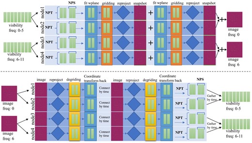
The diagram of gridding/degridding processes using WS-Snapshot and MFS.
WS-Snapshot Gridding Pseudo-code
 |
|
WS-Snapshot Gridding Pseudo-code
|
|
WS-Snapshot Degridding Pseudo-code
 |
|
WS-Snapshot Degridding Pseudo-code
|
|
We adopt the reproject_interp function from reproject package .3 The reproject package implements image reprojection (resampling) methods for astronomical images (Robitaille, Deil & Ginsburg 2020). The reproject package makes it easy to perform image projection in gridding and degridding with the correct PV2_1 and PV2_2 FITS keywords.
3 ALGORITHM ASSESSMENT
To further evaluate the usability of WS-Snapshot, we assessed its performance with simulated data.
3.1 Data preparation
We select SKA1-Low as the telescope for data simulation. All performance evaluations are based on the Measurement Set (MS) format generated by the simulated observations carried out by OSKAR4 (A GPU-accelerated simulator for the SKA). The main simulation parameters are listed in Table 2. The final MS file for evaluation is around 17GB, 5232 640 rows.
Simulation parameters used for OSKAR.
| Parameters | Values |
|---|---|
| Skymodel-1 | GLEAM |
| Skymodel-2 | Random faint source (FOV<5°) |
| Fainter source | Minimum flux 10−4 Jy |
| Telescope | SKA1-LOW full array |
| Phase_centre | RA: 0.0°, Dec.: −27.0° |
| Start_frequency_hz | 140 MHz |
| Num_channels | 30 |
| Frequency_inc_hz | 200 kHz |
| Channel_bandwidth_hz | 10 kHz |
| Observation length | 14 400 s |
| Num_time_steps | 40 |
| Time_average_sec | 0.9 s |
3.2 Evaluation environment
The evaluations were conducted on a small high-performance computing cluster with 13 nodes. All nodes have an Intel(R) Xeon(R) Gold 6226R CPU (32-core/64-thread) with 1024 GB memory and are connected by a 100 Gbps Infiniband network (EDR). All computer nodes were installed with Centos 7.9 Linux operating system with the newest updates, and Slurm 20.04 software was installed for task scheduling.
To investigate WS-Snapshot’s imaging performance and quality, we utilized a RASCIL-based continuum imaging pipeline (CIP) for the SKA telescope. IW-Stacking (Ducc.gridder) has been integrated into the CIP to perform the gridding/degridding and Fourier transform.
All evaluation scripts are written in python3, based on RASCIL version 0.5.0, Ducc.wgridder version 0.21.0, and Dask version 2022.1.0.
3.3 Computational performance
3.3.1 WS-Snapshot versus IW-Stacking
We first investigate the performance of the WS-Snapshot algorithm and analyse it in comparison with the IW-Stacking algorithm. The parameters evaluated in detail are shown in Table 3. To accurately evaluate the performance in the case of slicing at different observation times, we tested the cases of NPS equal to 1, 4, 8, and 20, respectively. For each of the NPS values, we evaluated the imaging performance at different scales such as 16 K (16, 384 × 16, 384), 24 K (24, 576 × 24, 576), and 32 K (32, 768 × 32, 768).
Scaling parameters.
| Parameters | Values |
|---|---|
| Scale | 16 K(5.5°), 24 K(8.2°), 32 K(10.9°) |
| NPS | 1, 4, 8, 20 |
| Number of threads | 8, 16, 24, 32, 40 |
| MFS channel | 6 (140 MHz-141 MHZ) |
| Parameters | Values |
|---|---|
| Scale | 16 K(5.5°), 24 K(8.2°), 32 K(10.9°) |
| NPS | 1, 4, 8, 20 |
| Number of threads | 8, 16, 24, 32, 40 |
| MFS channel | 6 (140 MHz-141 MHZ) |
Note. NPS = 12,16 are not divisible by 40 times and are not used in test.
The final evaluation results are given in Fig. 4. The time consumption of IW-Stacking is not related to the number of time slices but only to the image size. The time consumption of IW-Stacking gradually decreases as the number of threads grows, but the change is approximately stable after using 24 threads.
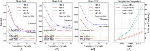
A, B, and C are the diagram of time consumption of WS-Snapshot and IW-Stacking (Ducc.wgridder) for different number of threads. D shows the relative complexity for Ducc and WS-Snapshot (NPS = 1) predictions and measurements as function of scales.
The time consumption variation of the WS-Snapshot algorithm is approximately the same as IW-Stacking. However, regardless of the value of NPS, most of the WS-Snapshot time consumption is better than IW-Stacking, and the trend of WS-Snapshot performance with the number of threads is also basically the same as IW-Stacking. WS-Snapshot significantly outperforms IW-Stacking for small NPS values and large scales. Regardless of the image size, a smaller NPS will significantly reduce the computational time, e.g. the minimum time consumption of WS-Snapshot is 450.3 s at 32 K with NPS = 1, and the minimum time consumption IW-Stacking is 2602.5 s. This means that WS-Snapshot is easier to achieve fine-grained parallelism with a sufficient number of compute nodes.
We tested the computation time of Ducc.wgridder and WS-Snapshot with different scales (i.e. 16 K, 24 K, 32 K), and then divided these computation times by the computation time of 16 K to obtain the computation time ratio. Similarly, we used the computational complexity equation in the Table 1 to predict 100 computational complexities within the scale from 16 K to 32 K. We also calculated the ratio of the predicted values to the predicted values for 16 K complexity. Fig. 4 (D) shows that the change in the ratio of computation time to prediction complexity is essentially the same. This also indicates that the complexity estimates are reasonable.
3.3.2 Comprehensive performance assessment
To evaluate the WS-Snapshot algorithm more objectively, we performed a comprehensive assessment of WS-Snapshot and IW-Stacking using the continuous imaging pipeline of SKA1-LOW. Assessment parameters such as different imaging sizes, number of threads, and NPS were considered in the evaluation (see Table 4). Likewise, we compared the imaging performance at different scales separately.
CIP test parameters.
| Parameters | Values |
|---|---|
| Scale | 16 K(5.5°), 24 K(8.2°), 32 K(10.9°) |
| NPS | 4 |
| Number of Taylor | 2 |
| Clean threshold | 1.2 × 10⁻³ Jy (>10 times minimum brightness) |
| Major cycle | 10 |
| Minior cycle | 10 000 |
| Input channels | 30 |
| MFS channel | 6 |
| Number of theads | 16 (for gridding/degridding) |
| Number of Dask-worker | 52 (13-nodes, 4 worker per node) |
Note. The number of channels in the data set is 30, generate one image for every 6 channels, output of 5 channels, represented by 2 taylor images.
During the assessment, we create 52 ‘Dask-workers’ on 13 computing nodes. Each node runs 4 ‘Dask-workers’. ‘Dask-scheduler’ is running on the first node of the cluster simultaneously.
Fig. 5 shows that compared with IW-Stacking (Ducc.wgridder), WS-Snapshot has a significant improvement in the combined processing performance, especially at the scale of 32K, WS-Snapshot can save nearly half of the time.
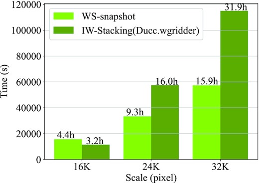
Histogram of CIP time consumption at different scales based on WS-Snapshot and IW-Stacking.
3.4 Imaging quality assessment
We carefully analysed the final imaging quality of the WS-Snapshot algorithm. We assessed the imaging quality in terms of both calculated dirty image and CIP results, using IW-Stacking imaging results as a comparison.
3.4.1 Imaging quality assessment
We subtracted the dirty images generated by WS-Snapshot and IW-Stacking at the same scale and NPS to obtain the difference images. The root means square error (RMS) is calculated for the difference images. The RMS for different scales with different NPS are given in Fig. 6.
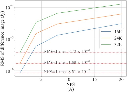
The RMS variations with different NPS.
As the NPS value increases, the RMS value increases from 10−6 to 10−4. As expected, larger imaging scales or larger NPS values will result in more significant errors.
To further assess the imaging quality, we set the NPS to 1, performed imaging calculations on the 40 observation times of visibility data included in the simulated MS, and then superimposed the generated 40 dirty images to generate the final dirty image (see Fig. 7). We further used the generated dirty image to subtract the dirty image produced by IW-Stacking to obtain difference images.
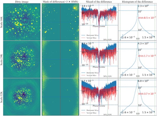
The dirty and the difference images and histograms of the difference are shown here for NPS of 1, three scales, with the horizontal and vertical slices of the difference image given, and the vertical coordinates of the difference slices and histograms are taken as log.
Due to the limited reprojection accuracy, the RMS of the edges is much higher than that of the central region in the difference image. It can also be seen from the histogram of the RMS that the central part of the image should be selected for the final image when high precision imaging is required.
3.4.2 Quality assessment of CIP results
To objectively compare the imaging quality, we evaluated the imaging results of both algorithms separately using the quality assessment (QA) procedure of the RASCIL QA tool (Lü et al. 2022), and the results are shown in Fig. 8. With the default parameters of RASCIL QA, the input fluxes are absolute and the output fluxes are apparent. The three results show that: (1) the source coordinate positions obtained by QA through the source search method are approximately the same, with differences in 2 per cent of error in both directions compared to the input source catalogue; (2) the spectral index of a source varies widely, with relatively small differences in brightness; and (3) the number of WS-Snapshot weak source detections is statistically consistent with IW-Stacking (within 101).
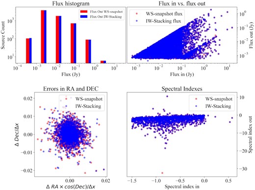
Comparison of WS-Snapshot and IW-Stacking (Ducc.wgridder) as gridder for CIP imaging quality evaluation at 32 K pixels 10 deg FOV. Up left: Histogram of the fluxes of all sources, binned logarithmically, where red and blue represents the output catalogue with two methods. Up right: The comparison of fluxs of all sources for input and output source catalogues. Bottom left: The errors between identified and input source positions, with respect to image resolution in (RA, Dec.). Bottom right: The comparison of spectral indexes for input and output source catalogues.
From the final imaging results, the 0th-order Taylor residual difference and the recovered image obtained from the CIP implemented by the two methods are approximately the same on flux, with the RMS of difference image as low as 10−5. The main difference is concentrated on the stronger point sources (as shown in Fig. 9, difference), which is also on the dirty image (Fig. 7, mask of the difference).
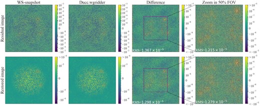
IW-Stacking (Ducc.wgridder) and WS-Snapshot are respectively applied to the 0th-order Taylor residuals image and the restored image of the CIP, and the corresponding difference (npixel:32 K, FoV:10.9 deg). Also shown here is a partial zoom of the snapshot dirty image of the bright source.
4 DISCUSSION
4.1 Reprojection
Reprojection plays a significant role in the overall WS-Snapshot implementation. Its performance also directly affects the performance of WS-Snapshot. However, the latest reproject package (version 0.8) cannot process a large-size image of 32 K up. Meanwhile, the reproject package is a serial implementation that significantly decreases the WS-Snapshot performance.
We optmized the ‘efficient_pixel_to_pixel_with_roundtrip’ function in the reproject package using multiple threads and keep the same number of threads as the gridding step for comparability of evaluation. With fewer than 32 threads, the time percentage of reproject increases with threads (as shown in Fig. 10).
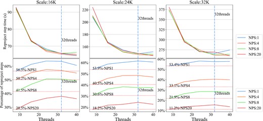
The figure shows the runtime and ratio of the reproject step of WS-Snapshot for single time slice with different parameters.
Although multithreading technology has been used, in calculating a single slice with NPS = 1, reproject takes up more than 50 per cent of the computation time. The optimization efficiency in the assessment has space for improvement. Currently, only the bottleneck step (’efficient_pixel_to_pixel_with_roundtrip’) is parallelized using python multithreading, and the interpolation and other steps remain based on the serial implementation.
4.2 Precision
WS-Snapshot can obtain a high degree of accuracy. Fig. 6 shows that in the best case (NPS = 1), the RMS of difference image is as low as 10−6, with the main differences from the image distortion due to the projection. In the worst case (NPS = 20), the error in the difference image reaches 10−4, a result that is unacceptable. This one shows that the value of NPS should be small when high accuracy results are needed.
It is necessary to note that it is also very difficult to further improve the accuracy of Ducc.wgridder. Ducc.wgridder can dynamically select the kernel, kernel support, and oversampling factor to obtain maximum performance, and we can specify the error (Arras et al. 2021) compared to the DFT by changing the epsilon parameter of Ducc.wgridder. However, adjusting this parameter in the Ducc.wgridder step of WS-Snapshot has no effect on the final results of WS-Snapshot because the main errors are caused by the image reprojection.
4.3 Network data transmission
Network transmission is an essential factor in the performance of distributed computing. The data that must be transferred between the various computing nodes in the CIP imaging computation is mainly visibility data and images. Image transfer is the main load in the computation, and the size of an image can reach 8 GB at a 32 K scale.
The visibility data is distributed as it is split by frequency first, then further in time slices. Therefore, each computing node needs to read about 223 MB of visibility data in the CIP at a 32 K scale.
After the computation is completed, we use the reduced form to implement image and visibility merging, which reduces the single node memory usage and increases speed.
5 CONCLUSIONS
After conducting various performance assessments, we conclude that WS-Snapshot has the following advantages in large-scale imaging.
Capable of achieving demanding wide-field imaging processing with the high accuracy required for scientific studies. The combination of W-stacking and Snapshot can guarantee sufficient accuracy in large-scale imaging processing (error range of 10−4 to 10−7). The central part of the image can be selected based on the FoV when high-precision imaging is required to avoid the errors caused by reprojections.
When using the fitted optimal plane, the value of w-range becomes smaller (see Fig. 2), which significantly improves the computational performance for IW-stacking (Ducc.wgridder). At a scale like 32 K, WS-Snapshot nearly halves the computation time.
Since the IW-stacking algorithm is splittable in u,v,w directions, WS-Snapshot can be computed for distributions of observations at different times. This makes sense for data processing on the scale of SKA.
Overall, WS-Snapshot inherits the advantages of the IW-Stacking and Snapshot methods. It can guarantee sufficient imaging accuracy and significantly reduce the runtime at large-scale imaging.
This study also shows that the bottlenecks encountered in the computation of WS-Snapshot deserve to be studied in more depth. These include how to perform the projection computation more quickly and with high accuracy and improve the performance of large-scale image computation.
ACKNOWLEDGEMENTS
This work was supported by the National SKA Program of China (2020SKA0110300), the Joint Research Fund in Astronomy (U1831204, U1931141) under cooperative agreement between the National Natural Science Foundation of China (NSFC) and the Chinese Academy of Sciences (CAS), the Funds for International Cooperation and Exchange of the National Natural Science Foundation of China (11961141001), the National Natural Science Foundation of China (No.11903009). The Innovation Research for the Postgraduates of Guangzhou University (2021GDJC-M13). The research of OS was supported by the South African Research Chairs Initiative of the Department of Science and Technology and National Research Foundation.
We do appreciate all colleagues of SKA-SDP ORCA and Hippo team for valuable and helpful comments and suggestions. This work was also supported by Astronomical Big Data Joint Research Center, co-founded by National Astronomical Observatories, Chinese Academy of Sciences and Alibaba Cloud.
DATA AVAILABILITY
We cloned RASCIL from its official repository and further implemented the WS-Snapshot. All the program code and part of the test data are stored in Gitlab repository, the RASCIL with WS-snapshot link is https://gitlab.com/ska-sdp-china/rascil.git, the link of the experimentally optimized reproject is https://gitlab.com/ska-sdp-china/reproject.git.
