


ABSTRACT
Young massive clusters (YMCs) are compact (≲1 pc), high-mass (>104 M⊙) stellar systems of significant scientific interest. Due to their rarity and rapid formation, we have very few examples of YMC progenitor gas clouds before star formation has begun. As a result, the initial conditions required for YMC formation are uncertain. We present high resolution (0.13 arcsec, ∼1000 au) ALMA observations and Mopra single-dish data, showing that Galactic Centre dust ridge ‘Cloud d’ (G0.412 + 0.052, mass = 7.6 × 10⁴ M⊙, radius = 3.2 pc) has the potential to become an Arches-like YMC (104 M⊙, r ∼ 1 pc), but is not yet forming stars. This would mean it is the youngest known pre-star-forming massive cluster and therefore could be an ideal laboratory for studying the initial conditions of YMC formation. We find 96 sources in the dust continuum, with masses ≲3 M⊙ and radii of ∼103 au. The source masses and separations are more consistent with thermal rather than turbulent fragmentation. It is not possible to unambiguously determine the dynamical state of most of the sources, as the uncertainty on virial parameter estimates is large. We find evidence for large-scale (∼1 pc) converging gas flows, which could cause the cloud to grow rapidly, gaining 104 M⊙ within 105 yr. The highest density gas is found at the convergent point of the large-scale flows. We expect this cloud to form many high-mass stars, but find no high-mass starless cores. If the sources represent the initial conditions for star formation, the resulting initial mass function will be bottom heavy.
1 INTRODUCTION
Young massive clusters (YMCs) are gravitationally bound stellar systems with masses ≳ 104 M⊙, radii ∼1 pc, and ages ≲ 100 Myr (Portegies Zwart, McMillan & Gieles 2010). The large number of co-eval stars within YMCs provide an important astrophysical laboratory to study the stellar initial mass function (IMF), stellar evolution, and stellar dynamics. As local Universe analogues of young globular clusters (Elmegreen & Efremov 1997; Kruijssen 2015; Pfeffer et al. 2018), studying nearby YMCs, provides an important way to understand the formation and early evolution of stars and clusters in extreme environments across cosmological time-scales.
Despite their importance, we still have limited observational examples of YMC progenitor clouds before star formation has begun (Ginsburg et al. 2012; Longmore et al. 2012; Urquhart et al. 2013; Contreras et al. 2017; Jackson et al. 2018). Two main YMC formation mechanisms have been proposed – a monolithic ‘in situ’ mode and a hierarchical ‘conveyor belt’ mode (see e.g. Longmore et al. 2014 for a review). In the monolithic scenario, all gas is contained within the final cluster volume before star formation begins. After forming its stars, the remaining gas is lost from the cluster, decreasing the global gravitational potential and the cluster expands towards its final, unembedded phase. In the hierarchical scenario, gas is initially more extended than the final cluster volume, with both the extended gas cloud and the embedded protostellar population undergoing global gravitational collapse simultaneously. Studies of young cluster and progenitor cloud populations show that the latter ‘conveyor belt’ formation mode, where gas accretion and star formation occur simultaneously, better reproduces their observed properties (Longmore et al. 2014; Walker et al. 2015; Krumholz & McKee 2020).
Observationally differentiating between these formation mechanisms is, however, difficult. A prediction of the hierarchical conveyor belt mode of YMC formation is that there should exist gas clouds with mass of 105 M⊙ and radii of a few pc, which contain a small amount of star formation activity. Without this on-going star formation it cannot be determined if a quiescent cloud will simply collapse to form a very high density proto-cluster in future (i.e. in situ). Identifying massive molecular clouds on the cusp of forming stars then provides the rare opportunity to observe the very initial stages of these YMC formation mechanisms, and provides insight to the dynamics of the cloud prior to the formation of stars.
Despite extensive observational searches (e.g. Bressert et al. 2012; Ginsburg et al. 2012; Urquhart et al. 2013; Longmore et al. 2013a, 2017), such clouds have remained elusive in the Milky Way. The most promising examples to date have generally been found in the ‘Central Molecular Zone’ (CMZ) – the inner few hundred pc of the Galaxy (Henshaw et al. 2022a) (the Henshaw + 22 references has been added in this edit). In particular, a region of the CMZ known as the ‘dust ridge’ (Lis et al. 1994), contains a collection of six massive (105 M⊙), compact (radius ∼1–3 pc), and largely quiescent clouds (excluding the Sagittarius B2 complex, one of the most active sites of high-mass star formation in the entire Milky Way, e.g. Ginsburg et al. 2018; Ginsburg & Kruijssen 2018; Schwörer et al. 2019) orbiting at ∼100 pc from the Galactic Centre (Kruijssen, Dale & Longmore 2015; Kruijssen et al. 2019a; Dale, Kruijssen & Longmore 2019a; Petkova et al. 2021) which have been identified as potential progenitors to YMCs (e.g. Longmore et al. 2013b; Rathborne et al. 2015; Walker et al. 2015; Barnes et al. 2019).
A subset of the dust ridge clouds have been studied in detail, from pc scales down to the scale of individual cores (∼1000 au) (e.g. Lis et al. 1994; Immer et al. 2012; Longmore et al. 2012, 2013b; Rodríguez & Zapata 2013; Rathborne et al. 2014, 2015; Mills et al. 2015; Walker et al. 2018, 2021; Barnes et al. 2019; Lu et al. 2019a,b, 2020, 2021; Henshaw et al. 2019, 2022b; Battersby et al. 2020; Hatchfield et al. 2020). Based on the evolution of dense gas structure and analysis of the gas kinematics, Walker et al. (2015, 2016) and Barnes et al. (2019) conclude that YMCs forming from these clouds are more likely to do so in a way that is more consistent with the predictions of a hierarchical conveyor belt mode. Intriguingly, Henshaw, Longmore & Kruijssen (2016c) observed a regular, corrugated velocity field – which they referred to as ‘wiggles’ – within the same contiguous gas stream as the dust ridge clouds, located ∼20 pc upstream from the dust ridge in projection. They found that the velocity extremes correlate with regularly spaced (∼8 pc) massive, compact molecular clouds. They interpreted the velocity wiggles as kinematic evidence of cloud formation via large-scale gravitational collapse. If this interpretation is correct, the dust ridge clouds are potentially more evolved, collapsing ‘wiggles’, providing a key laboratory for studying YMC formation.
Perhaps unsurprisingly given their important role for understanding star formation in extreme environments, the Galactic Centre gas clouds with signs of ongoing star formation activity have been studied in the most detail (e.g. Lu et al. 2019a, 2020; Walker et al. 2021). Unfortunately – at least as far as searching for a pre-star-forming YMC progenitor cloud is concerned – even the most massive and previously most quiescent of these, G0.253 + 0.016 (the ‘Brick’), has now been shown to be unambiguously forming stars (Walker et al. 2021; Henshaw et al. 2022b). Walker et al. (2021) find that this is only a small grouping of 18 low-to-intermediate mass sources, and is contained to a small area rather than widespread throughout the ‘Brick’. Henshaw et al. (2022b) find that the Brick may have already formed a small (∼103 M⊙) cluster.
In the ongoing search for a truly pre-star-forming YMC progenitor cloud, we therefore turn our attention to the least studied of the dust ridge clouds, G0.412 + 0.052 (hereafter referred to as cloud ‘d’). Despite having a similar mass and radius to other dust ridge clouds, cloud ‘d’ shows no signs of star formation on ≳0.01 pc scales (Walker et al. 2018; Barnes et al. 2019). In this study, we present high angular resolution (0.13 arcsec) (∼1000 au) ALMA Band 6 observations towards the peak of the single-dish continuum emission in cloud ‘d’ (clump ‘d6’ in Walker et al. 2018), using the same observational and spectral set-up as Walker et al. (2021) who found embedded star formation on 1000 au scales in the ‘Brick’. We aim to determine whether or not star formation is occurring at the scale of individual cores and understand the fate of this cloud by investigating the gas density distribution in relation to large-scale gas kinematics.
2 OBSERVATIONS AND DATA
2.1 Observations
We obtained single-pointing (Table 1), high-sensitivity and high-angular-resolution dust continuum and molecular line observations towards clump ‘d6’ in cloud ‘d’ with ALMA [RA (J2000) 17:46:23.0, Dec. (J2000) −28:33:23.5; Walker et al. 2018, see Fig. 1]. The observations were performed during ALMA’s Cycle 4 (project ID: 2016.1.00949.S, PI: D. Walker), at a frequency of ∼230 GHz (1.3 mm, frequency band 6). The angular resolution is ∼0.13 arcsec, which allows us to resolve scales of 1000 au, the scale of individual cores, at a distance of 8.1 kpc (Abuter et al. 2019). The observations contain 7 spectral windows, 5 of which targeted specific molecular transitions (Table 2) in the lower sideband with a spectral resolution of ∼0.77 km s−1. The remaining two spectral windows were dedicated to broad-band continuum detection in the upper sideband, with a spectral resolution of ∼2.5 km s−1. The total aggregate bandwidth is approximately 5.6 GHz. The project was observed across 4 individual execution blocks between October 2016 and April 2017. Each execution used 41–45 antennas, with baselines ranging from 15 to 3696 m. Full observation parameters and spectral set-up details can be found in Tables 1 and 2, respectively.
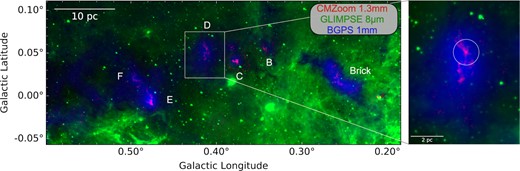
Left: Three-colour image of the Galactic Centre dust ridge. Red: SMA 1.3 mm dust continuum (Battersby et al. 2020), Green: Spitzer/GLIMPSE 8 μm emission (Churchwell et al. 2009), Blue: Bolocam Galactic Plane Survey 1 mm dust continuum (BGPS, Ginsburg et al. 2013). Right: Zoom-in on dust ridge cloud ‘d’ (G0.412 + 0.052) The white circle corresponds to the primary beam field of view of the ALMA observation towards source ‘d6’ (Walker et al. 2018) reported in this paper.
Details of the four observed execution blocks. Listed are the observation dates, nominal array configurations, number of 12 m antennas in the array, full range of antenna baseline lengths, total time on source, and the bandpass, flux, and phase calibrators used for each observation.
| Date | Array | Antennas | Baselines | Time on source | Bandpass | Flux | Phase |
|---|---|---|---|---|---|---|---|
| (d/m/y) | configuration | # | (m) | (min) | calibrator | calibrator | calibrator |
| 14/10/2016 | C40-6 | 41 | 18–2535 | 45.37 | J1924−2914 | J1924−2914 | J1744−3116 |
| 25/04/2017 | C40-3 | 41 | 15–450 | 27.22 | J1924−2914 | J1924−2914 | J1744−3116 |
| 19/07/2017 | C40-6 | 42 | 18–3696 | 45.37 | J1924−2914 | J1733−1304 | J1744−3116 |
| 08/08/2017 | C40-6 | 45 | 21–3696 | 45.37 | J1924−2914 | J1733−1304 | J1744−3116 |
Overview of the spectral setup used for our ALMA observation. The specific line(s) targeted per spectral window are given, along with the corresponding central frequency (νcent), bandwidth (BW), and spectral resolution in terms of velocity (Δν).
| Spectral | νcent | BW | Δν |
|---|---|---|---|
| window | (GHz) | (GHz) | (km s−1) |
| SiO (5–4) | 217.105 | 0.234 | 0.78 |
| H2CO (30, 3–20, 2) | 218.222 | 0.234 | 0.78 |
| H2CO (32, 2–22, 1) | 218.476 | 0.234 | 0.78 |
| H2CO (32, 1–22, 0) | 218.760 | 0.234 | 0.78 |
| 13CO (2–1)/CH3CN (12–11) | 220.709 | 0.934 | 0.77 |
| Continuum | 232.500 | 1.875 | 2.50 |
| Continuum | 235.000 | 1.875 | 2.47 |
2.2 Image cleaning and processing
The ALMA pipeline calibrated data sets for each execution block were combined to obtain final data products, which were then imaged in casa version 5.6.0.68 (McMullin et al. 2007).
Prior to generating the dust continuum, any channels with spectral-line contamination were flagged. No line emission is detected in the broad spectral windows in the upper sideband, and only a small fraction of the channels in the other spectral windows contain line emission. We estimate that no more than 10 per cent of the aggregate bandwidth is flagged due to line contamination, and the effective bandwidth used for continuum generation is ∼5 GHz.
We use casa’s tclean task to image both the continuum and line cubes. Due to the complex structure of cloud ‘d’, we opt for tclean’s ‘automasking’ mode over 105 iterations. A cleaning threshold of 15 |$\mu$|Jy (the rms sensitivity of the continuum image) was used, with Briggs weighting and a robust parameter of 0.5. The resultant image has a synthesised beam size of 0.14 arcsec × 0.11 arcsec (∼1100 au × 890 au).
We note that some of our initial ALMA data is lost due to the different footprints of the feathered data sets. We do not, however, lose any of the main area of dust emission, and so continue with this feathered image.
After feathering, the rms continuum sensitivity is ∼15 |$\mu$|Jy, corresponding to a 5σ mass sensitivity of ∼0.1 M⊙, assuming a dust temperature of 20 K (see Section 3.1).
We split out the target spectral windows using casa’s split task and defining the spectral windows that are our desired targets. We subtract the continuum from the isolated lines using the uvcontsub task. We use the tclean task to image the lines. We use the interactive manual clean so we can stop defining masks when all the emission had been cleaned and the residuals look like noise with no remaining structure. We again use Briggs weighting and a robust parameter of 0.5, although here we use a cleaning threshold of 0.06 mJy. Finally, we use the immoments task to produce the desired moment maps.
For the spectral lines, we only have 12m data, and so we are missing the larger scale structure. We use casa’s imsmooth task to perform a spatial Gaussian smoothing on the molecular line data to improve the signal-to-noise ratio. We set the major and minor axes parameters of the Gaussian smoothing kernel to equal ∼0.34 arcsec, double the size of the major axis of the synthesized beam. This increased the rms of the line images from ∼0.6 to ∼1 mJy. Any discussion regarding molecular lines hereafter refers to results obtained from this Gaussian smoothing. The resulting moment maps of the lines following this smoothing can be found in the supplementary online material. We will discuss the morphology and kinematics of this emission later in the paper.
3 RESULTS
3.1 Spatial distribution, mass, radius, and density of compact continuum sources
The left-hand panel of Fig. 2 displays the ALMA-only 1.3 mm dust continuum map for cloud ‘d’, focused on ‘d6’ (Walker et al. 2018), along with overlaid contours of both the feathered continuum data (red) and the combined SMA and Bolocam Galactic Plane Survey (BGPS) data (black; Walker et al. 2018). The right-hand panel displays the continuum map for our data feathered with ALMA+BGPS data (Barnes et al. 2019), with the same contours as the left-hand panel. Note that a section of the feathered continuum map is missing on the upper right side due to the ALMA data and the ALMA+BGPS data having different footprints. However, no obvious structure has been lost in this process (see the left-hand panel of Fig. 2 for the unfeathered ALMA data with a complete footprint). We detect dense substructure within cloud ‘d’ with a filamentary morphology. The mass concentration peaks in the middle of the image, which corresponds to the peak of the continuum emission in the lower resolution images.
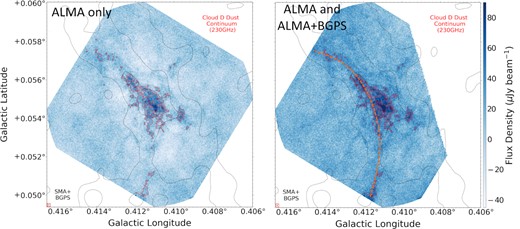
Left: Dust continuum map of our ALMA data only. Red contours show structure in the continuum data at levels of 45, 60, and 80 |$\mu$|Jy (levels of 3, 4, and 5.3σ, respectively). Black contours show just the SMA+BGPS continuum data from Walker et al. (2018). The black circle in the bottom left (highlighted by a red box) represents the synthesized beam. Filamentary structure is not as clear in the unfeathered data. Additionally, white ‘patches’ can be seen surrounding the filament. These ‘negative bowls’ are a sign of missing zero-spacing data (i.e. the large-scale structure has been spatially filtered out). Right: Our ALMA data feathered with ALMA+BGPS data (Barnes et al. 2019). Red contours show structure in the continuum data at levels of 45, 60, and 80 |$\mu$|Jy. Black contours show just the SMA+BGPS continuum data from Walker et al. (2018). The black circle in the bottom left (highlighted by a red box) represents the synthesized beam. Curved filamentary structure (represented by a dashed orange line) can be seen with a roughly central mass concentration. A section of the map is missing due to our ALMA data and the Barnes et al. (2019) ALMA+BGPS data having different footprints.
Dendrograms pick out substructures as independent entities in a hierarchical manner, with the smallest possible structures being referred to as ‘leaves’. The dendrogram leaves are shown in Fig. 3, with each red contour indicating substructure detected using the above parameters. In the context of this research, each leaf is a potential star-forming core of the scale ∼103 au (Table A1). Using these dendrogram parameters, we isolate 96 compact continuum sources. We have varied the parameters of the dendrogram to see how this affects our results, namely by increasing the threshold to 5σ. In this case, we detect nine sources as opposed to 96. We repeat our analysis on just these nine sources detected over 5σ and report our results for comparison, but for completeness we show the properties of all 96 3σ sources.
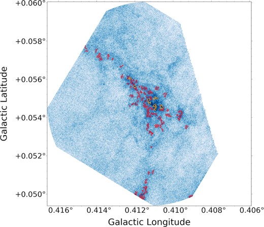
Locations of dendrogram leaves extracted with the ASTRODENDRO code. The dendrogram was computed using a threshold of 3σ (σ = 16 |$\mu$|Jy), an increment of σ and an Npix value of 77. Red contours show the individual compact continuum sources (‘leaves’) isolated by the dendrogram, of which 96 are found. Yellow contours show the nine continuum sources detected above 5σ. Note that some of the leaves extend beyond the boundary of the observed region, and so these are later excluded from analysis.
Given the large mass of gas it is perhaps surprising that most of the structure has a column density only 3–5σ above noise. This makes it difficult to determine whether an individual dendrogram leaf is a physically distinct object or not – the nature of these sources is uncertain. However, it leads to one of the main conclusions of this paper, that the column density contrast in the cloud is very small. The lack of density contrast on 1000 au scales in this cloud is reminiscent of the lack of density contrast found at 0.1 pc scales throughout the CMZ in Battersby et al. (2020).
We also need to assume the dust temperature in order to estimate masses. We use a dust temperature of ∼20 K, based on estimates by Tang, Wang & Wilson (2021). The uncertainties in the dust temperature and opacity mean that systematic uncertainties in the mass estimates are a factor of ∼2 (Kauffmann et al. 2008).
Additionally, we have assumed a spectral index, β, of 1.75 (Battersby et al. 2011). It should be noted that recent estimates by Tang et al. (2021) determine β in the CMZ to be in the range of 2.0–2.4 on scales of 10.5 arcsec. Using the upper value of this range of β = 2.4 instead of our assumed value of 1.75 increases our reported masses by a factor of ∼1.69. Additionally, Marsh et al. (2017) use Herschel data to create higher resolution maps (12 arcsec) using the PPMAP procedure, reducing the average dust temperature to ∼17 K. If we assume this dust temperature and combine it with β = 2.4, then our reported masses would increase by a factor of ∼2.10. Therefore, our mass and density estimates, using a β value of 1.75 and dust temperature of 20 K, may be underestimates. These measures of temperature and β are on significantly larger scales than we are probing, so any variations on smaller scales are not well constrained.
We also note that, as discussed in Rosolowsky & Leroy (2006), sources extracted via a contour-based extraction technique often have intrinsic sensitivity and resolution biases. Interferometers systematically underestimate cloud properties, particularly the flux and by extension the mass. For example, Rosolowsky & Leroy (2006) find that the flux of Orion is underestimated by 5 per cent even at high sensitivity. Therefore, our mass estimates could also be underestimates by a factor of 0.05 due to this.
We calculate effective radii for each structure by calculating the radius of a circular source with an area equal to that of the structure (|$R_\mathrm{eff} = \sqrt{A/\pi }$|, where A is the area enclosed within the dendrogram boundary). Using the calculated masses and effective radii, we then compute the volume densities of the sources, assuming a spherical geometry.
We have assumed that all flux within each dendrogram leaf belongs to the cloud ‘d’ continuum sources. However, the case may be that some flux in each leaf is background emission. To account for this, we have calculated background-subtracted fluxes, masses, and densities for each leaf. To do this, we use the minimum pixel value in each leaf as a proxy for the background emission (Pineda et al. 2015; Henshaw et al. 2016b). We then subtract this value from each pixel in the leaf and then find the total flux after this subtraction. We then use these flux values to calculate background-subtracted masses and densities.
On average, the continuum sources with background-subtraction are ∼9 times less massive and dense than the non-background-subtracted continuum sources. This is likely due to the contrast within each leaf being small, and so even subtracting the minimum value integrated over the leaf is quite significant. In the rest of our analysis, we use the non-background-subtracted masses and densities, but we acknowledge that these could be overestimates if any flux in the continuum sources does not belong to the source itself.
The mean mass, radius, and number density of the 96 compact continuum sources are 0.67 M⊙, ∼1.6 × 10³ au and 7.1 × 106 cm−3, respectively, all computed from within the footprint of the dendrogram leaf. The total combined mass of the sources is 65 M⊙. Repeating this analysis for the nine sources detected above 5σ gives a mean mass, radius, and number density of 0.94 M⊙, ∼1.6 × 10³ au and 9.7 × 106 cm−3, respectively, with a total combined mass of 8.4 M⊙. A table of these values (and background-subtracted values) for each source can be found in the Appendix (Table A1). We discuss the implications of these masses in Section 4.
3.2 Search for star formation tracers within cloud ‘d’ continuum sources
We searched for 13CO, CH3CN, and SiO emission towards the cloud ‘d’ continuum sources. 13CO is a commonly used tracer for outflows due to its high abundance and relatively low energies of the lower rotational states (Bally 2016). CH3CN is used to trace small-scale gas kinematics towards hot protostellar cores, and the relative intensities of the k-components can be used to estimate gas temperatures and column densities (e.g. Beuther et al. 2017; Ilee et al. 2018; Maud et al. 2018). SiO is a well-known tracer of proto-stellar outflows. Walker et al. (2021) detected both strong CH3CN emission and SiO outflows towards the young, low-mass star-forming cores in the ‘Brick’. However, we do not detect any CH3CN emission towards the continuum sources, nor do we detect any SiO outflows. We searched for SiO outflows by manually inspecting every channel in the SiO cube and although we detect SiO emission, no distinct outflow morphology can be seen. 13CO is detected, but the emission is widespread (see the integrated intensity maps in the supplementary online material) with no distinct outflow structure. Cloud ‘d’ also shows a lack of Class II methanol and water maser emission (Cotton & Yusef-Zadeh 2016; Rickert, Yusef-Zadeh & Ott 2019; Lu et al. 2019a) and 70 |$\mu$|m emission (Herschel, HiGAL; Molinari et al. 2010), both tracers of star formation. Cloud ‘d’ does not show any detections of radio continuum emission from possible H ii regions (Immer et al. 2012; Lu et al. 2019a), nor does it show any 24 or 8 |$\mu$|m emission (Churchwell et al. 2009).
In summary, even with the order of magnitude improvement in angular resolution and sensitivity provided by ALMA, cloud ‘d’ remains unique among the dust ridge clouds in still having no signs of star formation.
3.3 Nearest neighbour analysis of compact continuum source separations
In order to calculate the separations of the compact continuum sources within cloud ‘d’ and compare them to theoretically predicted values, we carry out nearest neighbour analysis using the scikit-learn module neighbors. We use a n_neighbors parameter of 2 and set the algorithm parameter to auto. From this analysis, we find that the nearest neighbour separation between continuum sources in cloud ‘d’ is typically of the order 103 au. Most continuum sources have a nearest neighbour separation of less than ∼7.5 × 10³ au, with a mean of ∼2.6 × 10³ au.
However, this number is not the mean separation between sources. Kruijssen et al. (2019c) show that the expectation value of the nearest neighbour distance is |$\langle r_n \rangle = \sqrt{\pi }\lambda /4 \approx 0.443\lambda$|, where λ is the mean separation length. This expression is the integrated form of the probability distribution function of the nearest neighbour distance. Rearranging this expression for λ means that we must multiply the mean nearest neighbour separation by a factor of ∼2.3 to get the mean separation length.
This separation is also the 2D projection of the nearest neighbours, and we do not know the complete 3D separation. The implicit assumption is then that the sources all lie in the same 2D plane of the sky. In reality, the sources will also lie at different distances along the line of sight, so the separations between them may appear smaller than they are in reality due to projection effects. To correct for this, we also multiply the mean nearest neighbour separation by |$\sqrt{3/2}$|. This is based on the reduction of three dimensions to two, that is (x2 + y2 + z2) to (x2 + y2).
Combined with the earlier factor of 2.3, this means we must multiply our mean nearest neighbour separation by a factor of ∼2.8. Converting each nearest neighbour separation to a separation length gives a mean separation length of ∼1.5 × 10⁴ au. Separation lengths are shown in Fig. 4. Below we compare this to the expected gas fragmentation scale.
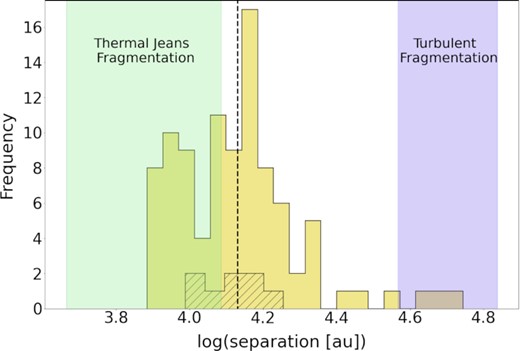
The separations of the 96 individual continuum sources, calculated using nearest neighbour analysis and corrected for geometric and projection effects. The black hatched histogram shows the same quantity for the nine 5σ sources. The black dashed line shows the mean separation. The green shaded region represents the range of predicted thermal Jeans lengths and the blue shaded region represents the range of predicted turbulent Jeans lengths. The separation between compact continuum sources in cloud ‘d’ is typically of order 104 au, with a mean of ∼1.5 × 10⁴ au and a standard deviation of ∼8.0 × 10³ au. The separations of the continuum sources lie between thermal and turbulent fragmentation predictions.
Compared to the disc of the Galaxy, the CMZ has an elevated gas temperature (60 K versus 10 K; Ginsburg et al. 2016; Immer et al. 2016; Krieger et al. 2017) and velocity dispersion (5 km s−1 versus 1 km s−1 at a fixed size-scale, Shetty et al. 2012). Therefore, we expect that the thermal and turbulent fragmentation scales in the CMZ will be different to those in the disc.
If the gas and dust are thermally coupled, then we expect the gas temperature to be ∼20 K, matching the dust temperatures reported by Immer et al. (2012) and Walker et al. (2015) of 17−23 K (Clark et al. 2013). However, on larger scales, the gas and dust are often thermally decoupled (e.g. Ginsburg et al. 2016; Immer et al. 2016). The only gas temperature constraint on similar spatial scales in this cloud is from Walker et al. (2018) and is an upper limit of ∼60 K, based on the non-detection of higher excitation H2CO transitions towards clump ‘d6’. Based on this, we use upper and lower limits of 20 K and 40 K. We choose 40 K as a reasonable upper limit as we do not have a firm constraint on the actual temperature, and this temperature is lower than the estimated upper limit.
Using both of these gas temperature estimates, as well as both estimates of mass, we derive thermal Jeans length estimates of λJ, therm = 8.0|${}^{+4.2}_{-3.4}$| × 103 au. The expected value of the turbulent Jeans fragmentation length is λJ, turb = 5.3|${}^{+1.6}_{-1.6}$| × 104 au. Fig. 4 shows the distribution of the separations, along with the mean value (black dashed line) and the ranges of the thermal and turbulent fragmentation lengths (shaded regions). The mean separation of 1.5 × 10⁴ au lies between these ranges, meaning it is potentially consistent with both, although marginally more consistent with thermal Jeans fragmentation. When making this comparison for the nine sources found above 5σ, we again find that the separations are still marginally more consistent with thermal Jeans fragmentation, with no separations being consistent with turbulent Jeans fragmentation. The mean separation, however, still lies between the two predictions, with a mean value of 1.3 × 10⁴ au.
Repeating this analysis but using a value of half the thermal Jeans and turbulent Jeans fragmentation wavelengths (to represent the fact that fragments may form at half-wavelength-spaced nodes), the distribution marginally favours the turbulent fragmentation length. However, given the large uncertainty in these measurements, we conclude the data are consistent with both predictions. Therefore, it is not possible to unambiguously distinguish whether the separation distribution is more likely to be drawn from a thermal Jeans or turbulent Jeans fragmentation mechanism.
The estimated thermal Jeans mass is MJ, therm = 0.54|${}^{+0.70}_{-0.35}$| M⊙. The estimated turbulent Jeans mass is MJ, turb = 144|${}^{+43}_{-43}$| M⊙. Therefore, the masses of the sources (see Table A1) are roughly consistent with the predicted thermal Jeans mass limits of the clump and not with the turbulent Jeans mass predictions. When making this comparison for the nine sources found above 5σ, we find the same trend – the majority of sources are consistent with thermal Jeans mass estimates, with a few lying at masses greater than this.
In summary, the consistency of the source masses with thermal Jeans mass estimates, along with the slight tendency of the separations towards thermal Jeans fragmentation, it seems as though thermal Jeans fragmentation is a better descriptor of the source structure in this cloud. This is consistent with recent results from Lu et al. (2020) and Walker et al. (2021).
3.4 Virial analysis of cloud ‘d’ continuum sources
We produce spectra towards each of the continuum sources (see supplementary materials) in SiO and three different H2CO transitions. To produce these spectra, we extract an averaged spectrum for each leaf in the dendrogram. We then use the pyspeckitpython package to fit each these spectra with a Gaussian profile in order to obtain velocity dispersions. We set the guesses parameter as the amplitude is equal to the maximum amplitude within the spectrum, the velocity is equal to the velocity at the point of highest amplitude, and the width is equal to full width at half-maximum of the line. We note that only H2CO effectively traces the mass (see supplementary online material), and so we only use the lowest energy formaldehyde transition in later analysis.
For the majority of continuum sources, we could not measure an appropriate velocity dispersion, and the ones that we could measure have large measurement uncertainties. For continuum sources where we could measure reliable velocity dispersions, we calculate α values in the range of 5|${}^{+13}_{-4.94}$|–45|${}^{+55}_{-33}$| (see Table A2 in the Appendix for a full list of these calculated values). All of the calculated values are greater than 2. However, their uncertainties mean that some may have a virial parameter of less than 2. Therefore, assuming that these values are representative of the whole sample of continuum sources, it may be the case that some of the continuum sources in cloud ‘d’ are gravitationally bound, but uncertainties on the velocity dispersions of the continuum sources mean that in practice the virial state of the sources is essentially unconstrained.
Virial parameter, α, and velocity dispersion, σ, (and associated upper and lower limits) of sources for which velocity dispersion could be measured in H2CO (30, 3–20, 2). Asterisks denote the sources found using a 5σ threshold.
| Source | α | αlower | αupper | σ | Δσ |
|---|---|---|---|---|---|
| Number | H2CO (30, 3–20, 2) | (km s−1) | (km s−1) | ||
| 19 | 8.353476 | 2.099979 | 18.760553 | 0.752865 | 0.375388 |
| 22 | 27.004411 | 2.600424 | 77.09842 | 1.023652 | 0.705996 |
| 29 | 10.909824 | 0.106466 | 39.434801 | 1.030012 | 0.928261 |
| 30 | 10.468572 | 3.335144 | 21.574139 | 1.055967 | 0.459943 |
| 50 | 44.978999 | 11.594935 | 100.162932 | 1.289734 | 0.634902 |
| 55 | 12.351154 | 0.910142 | 36.903537 | 0.761981 | 0.555136 |
| 56 | 5.417488 | 0.81414 | 14.083529 | 0.586945 | 0.35941 |
| 58 | 25.066655 | 7.456437 | 53.037347 | 1.419999 | 0.645527 |
| 79 | 29.780918 | 5.930561 | 71.895217 | 1.199221 | 0.664068 |
| 80* | 6.147653 | 1.128015 | 15.185141 | 0.846895 | 0.484124 |
| 81 | 22.668 | 5.600116 | 51.204446 | 0.923663 | 0.464565 |
| 82 | 5.119289 | 0.055064 | 18.408492 | 0.732269 | 0.656324 |
| 85 | 12.289794 | 4.493792 | 23.926809 | 0.914435 | 0.361484 |
If we use only the nine 5σ sources detected, then only one of the sources has reliable H2CO emission. Therefore, we continue virial analysis with the full 96 source sample, as this still leaves the virial state of the sources unconstrained and ultimately does not change our conclusions.
This analysis of the virial parameter faces a potential issue, in that H2CO emission is extended. When we extract the spectrum towards continuum sources, it is important to distinguish the relative contribution from the compact continuum source and larger scales. Including emission from gas not associated with the source will affect the inferred gravitational boundedness. However, we do know that the formaldehyde and dust emission have good spatial correspondence, so we assume that this effect is minimal. Additionally, while H2CO is extended, it is used as a reliable tracer of dense gas kinematics in the CMZ (e.g. Walker et al. 2018; Lu et al. 2021), and so we consider it a reliable tracer of velocities.
To investigate the virial state further, we find the elongation of each continuum source by calculating the ratio of the major axis to the minor axis. We expect that unbound structures will have a higher degree of elongation than bound structures. This is because gravitationally bound structures would appear roughly circular due to being roughly spherical, whereas unbound structures are less likely to appear circular. We find ratios in the range of 1–4.5, with a mean value of ∼1.92. We also plot the virial parameter against the aspect ratio (Fig. 5) to see if continuum sources with a lower virial parameter correspond to a smaller aspect ratio. However, there is no clear correlation.
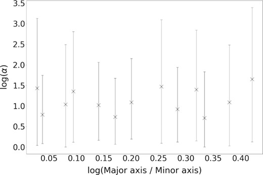
Comparison of the virial parameters of the continuum sources for which we could measure reliable velocity dispersion and their aspect ratios. One might expect continuum sources with a lower virial parameter (i.e. more likely to be gravitationally bound) to be more circular, but there is no correlation between these parameters.
In Section 4.3, we discuss the possibility of these continuum sources also being in pressure-bounded equilibrium.
4 DISCUSSION
Dust ridge cloud ‘d’ is one of the most massive (104−5 M⊙) and compact (R ∼ 3 pc) molecular clouds known to exist in the Galaxy in which there are no known signs of local or widespread star formation. Our ALMA observations towards the highest density region of the cloud confirm that there is no evidence of active star formation in the form of outflows or gas tracers down to protostellar scales (1000 au).
Our analysis of the continuum emission reveals an overall lack of compact substructure in the cloud. We identify a population of 96 low-mass continuum sources, for which the gas structure is more likely to be set by thermal fragmentation rather than turbulent fragmentation (Fig. 4). In Section 3.4, we found that the majority of these continuum sources are unlikely to be gravitationally bound ‘cores’. Moving forwards in the paper, we will therefore continue to refer to them as ‘sources’.
Nearest-neighbour analysis has shown that the sources have separations consistent with both thermal Jeans and turbulent Jeans fragmentation, with a tendency towards thermal. Additionally, the masses of the sources are consistent with the predicted thermal Jeans mass of the cloud. Several recent studies (Lu et al. 2019a, 2020; Walker et al. 2021) have found that separations are consistent with thermal Jeans fragmentation in other CMZ clouds, including the ‘Brick’.
This suggests that, while turbulence drives gas properties on large-scales in the CMZ, smaller scales may be less sensitive to this. On protostellar scales, star formation in the CMZ may proceed in a similar way to star formation regions in the local neighbourhood, albeit with a higher critical density threshold to overcome before star formation can begin (Walker et al. 2018; Barnes et al. 2019).
Fig. 6 shows a mass distribution of the sources. Compared to a standard core mass function, the distribution is bottom-heavy and has no high-mass progenitors – the most massive source is ∼3 M⊙, the mean mass of ∼0.7 M⊙, and most sources being <1 M⊙. If these sources are the precursors to stars, in order for the resulting stellar distribution to conform to a normal IMF, the compact continuum sources must gain many times their current gas mass from the surrounding environment. Calculating the mass distribution for the nine sources detected above 5σ, the majority of sources are still <1 M⊙, meaning they would still have to accrete a large amount of material from the surrounding environment. However, in both cases, not much can be said about the slope of this mass distribution as there are not enough sources to build a statistically meaningful mass function.
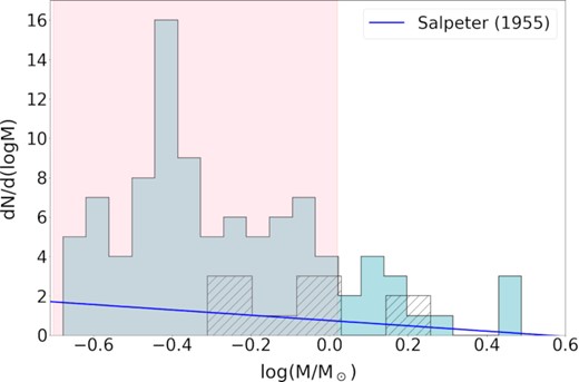
Mass distribution of the 96 individual sources detected by our dendrogram analysis. The black hatched histogram shows the same quantity for the nine 5σ sources. The Salpeter (1955) IMF is overplotted (blue line). The pink shaded region shows the range of predicted thermal Jeans masses for the clump, for which most masses are consistent.
Coupled with the lack of molecular line emission tracing hot cores or outflows, our results paint a coherent picture of a massive molecular cloud with no signs of star formation. In the following, we compare our results with complementary data to investigate the ultimate fate of this extreme molecular cloud.
4.1 Do the properties of sources vary with environment?
On global (1−100 + pc) scales in the CMZ, gas conditions are known to be extreme compared to the Solar neighbourhood. Densities (∼103−4 cm−3, Guesten & Henkel 1983; Mills et al. 2018), gas temperatures (typical gas temperatures are 50−100 K, but can reach as high as 400−600 K, Mills & Morris 2013; Ginsburg et al. 2016), pressures (P/kB ∼ 107−9 K cm−3, Longmore et al. 2014; Rathborne et al. 2014) and line widths (∼10−20 km s−1, Henshaw et al. 2016a) are between several factors to several orders of magnitude greater than those found in the disc. It is therefore plausible that the star formation process may occur differently in such an environment. To investigate this on protostellar (1000 au) scales, we compare the properties of the sources detected in cloud ‘d’ and compare them with cores both in the CMZ and the Galactic disc.
We take fig. 3 from Walker et al. (2018), which shows the mass–radius plot for a sample of CMZ and disc cores from the literature, and add our 96 sources. Also plotted are Walker et al. (2018)’s 15 SMA clumps and the cloud ‘a’ core (aka the ‘maser core’ in the ‘Brick’) mass and radius from Rathborne et al. (2014). The plot also includes a sample of high-mass protostellar cores found in the Galactic disc, taken from Peretto et al. (2013), as well as high-mass protostellar cores in the W43-MM1 ridge, a likely precursor to a ‘starburst cluster’, taken from Louvet et al. (2014). The masses of these cores have been scaled to make them consistent with the spectral index of β = 1.75 that we have used for mass estimates in our analysis. We have also plotted masses and radii for multiple CMZ cores from Lu et al. (2020) and the masses and radii of eighteen cores in cloud ‘a’ (aka the ‘maser core’ in the ‘Brick’/G0.253 + 0.016, Walker et al. 2021). The masses and radii of the cores in these samples were both calculated in the same way as the ALMA sources, assuming the same dust temperature of 20 K, and so direct comparison is possible. The resulting plot is shown in Fig. 7.
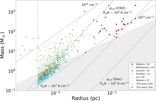
Mass–radius plot for all of the compact continuum sources reported in our ALMA sample. The solid cyan diamonds correspond to masses of the 96 sources detected above 3σ, estimated assuming a dust temperature of 20K. Solid pink diamonds show the same quantity for the nine sources detected above 5σ. Solid red squares correspond to SMA clump upper mass limits reported in Walker et al. (2018). The red point with a black star marker indicates the clump from Walker et al. (2018)’s sample that we have observed in this work. Black points correspond to high-mass protostellar cores in the Galactic disc taken from Peretto et al. (2013) and blue triangles to those from Louvet et al. (2014). The open red square corresponds to the star-forming core in cloud ‘a’ (aka the ‘Brick’) as seen with ALMA observations (Rathborne et al. 2014). Green crosses represent cores within four CMZ clouds as seen with ALMA observations (Lu et al. 2020) and yellow points correspond to cores found within cloud ‘a’ by Walker et al. (2021). Dash/dot lines show constant column density. Dashed lines show the predicted critical volume density thresholds for both the CMZ and the Galactic disc, assuming pressures of P/k = 109 and 105 K cm−3, respectively, with an intermediate threshold for a pressure of P/k = 107 K cm−3. The red dashed line corresponds to our resolution of ∼1000 au. The area above the grey-shaded region corresponds to the portion of the mass–radius plane above the empirical high-mass star formation threshold proposed by Kauffmann & Pillai (2010).
We find that the sources detected in cloud ‘d’ are consistent with the mass–radius relationship of cores detected in star-forming clouds in both the CMZ and the disc, though the cloud ‘d’ sources are on the lower end of the mass distribution at a given size scale. The area above the grey-shaded region of Fig. 7 corresponds to cores which lie above the empirical massive star formation threshold proposed by Kauffmann & Pillai (2010), which they determine to be M(R) ≳ 870 M⊙ × (R/pc)1.33. We find that all of the cloud ‘d’ sources are below this limit, and therefore should not be forming high-mass stars. Assuming that the sources are not transient and continue to accrete mass, they may eventually exceed this threshold and begin forming stars. However, as Kauffmann & Pillai (2010)’s threshold was derived for clouds in the Solar neighbourhood, it is unclear whether this should hold in the CMZ. Indeed, Walker et al. (2018) find that all of their CMZ clumps are on or above this limit, but only two show signs of star formation. At the scale of our ALMA data, it is difficult to conclude whether or not there is an environmental dependence on star formation, as none of our sources are above the threshold.
4.2 Are the sources in hydrostatic equilibrium?
Although the virial ratios calculated in Section 3.4 suggest the sources may not be self-gravitating, previous observations have suggested dense gas sources in the CMZ may be in hydrostatic equilibrium but confined by the high ambient pressure in the CMZ. We follow the analysis of both Field, Blackman & Keto (2011) and Walker et al. (2018) to investigate this possibility in cloud ‘d’. Field et al. (2011) study Galactic disc clouds from the Galactic Ring Survey (GRS; Jackson et al. 2006) as self-gravitating isothermal spherical clouds, subject to a uniform external pressure Pe, in the context of the virial theorem. Based on the GRS analysis of Heyer et al. (2009), the disc clouds are not bound when considering simple virial equilibrium. Field et al. (2011) find that external pressures of Pe/k ∼ 104−6 K cm−3 acting upon the clouds are needed for them to be in pressure-bounded equilibrium.
Walker et al. (2018) expanded on the Field et al. (2011) analysis by comparing their SMA observations of dust ridge clouds and clumps with the disc clouds. They conclude that, if these dust ridge clouds and clumps are in pressure equilibrium, then the external pressures in the CMZ would have to be of order Pe/k ∼ 108 K cm−3, 2–3 orders of magnitude greater than necessary for the clouds in the Galactic disc. This is consistent with the measured ambient pressure in the CMZ of Pe/k ∼ 107−9 K cm−3 (Kruijssen et al. 2014; Longmore et al. 2014; Rathborne et al. 2014).
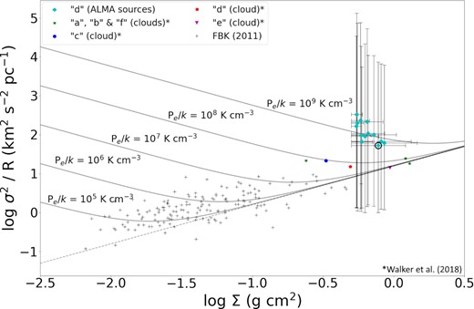
Comparison of the dust ridge sources with dust ridge clouds and GRS clouds. Black crosses show disc clouds as reported in Field et al. (2011) (original data from Heyer et al. 2009). Diamond-shaped markers indicate the cloud ‘d’ sources. The data point circled in black is the only source that was detected above 5σ that also had reliable H2CO emission. All other solid markers indicate dust ridge clouds, as reported in Walker et al. (2018). Curved black lines are those of constant external pressure, while the dashed line is for Pe = 0.
From Fig. 8, we can see that the pressures required to confine sources on the scale of these sources are ∼109 K cm−3. This is an order of magnitude larger than the external pressures determined for the large-scale clouds by Walker et al. (2018). This suggests that there is either an additional confining pressure on source scales that is undetected in cloud scale observations, or that the sources are overpressured with respect to the surrounding gas and are therefore transient.
The densities of these sources are of the range 106−7 cm−3, 2–3 orders of magnitude greater than the volume density threshold proposed by Lada, Lombardi & Alves (2010). Despite this, and the high external pressures the sources are subject to in the CMZ, the sources show no signs of star formation. We conclude that this is further evidence for star formation being inhibited in the CMZ due to the critical volume density threshold for star formation being driven up by the high turbulent energy density in this environment (Kruijssen et al. 2014; Rathborne et al. 2014).
4.3 Evidence for convergent gas flow
The lack of star formation in cloud ‘d’ indicates one of two scenarios – either cloud ‘d’ is in the very early stages of cluster formation, or it will never form a cluster at all. Given the high gas density (|$n_{\rm H_2}$| = 0.7 × 105 cm−3, tff = 11.4 × 10⁴ yr; Barnes et al. 2019), the fact the cloud and the dense clumps (at the scale Reff ∼0.1 pc) within it are gravitationally bound (Longmore et al. 2013b; Barnes et al. 2019), and the short free-fall times at all scales (Barnes et al. 2019), the latter of these scenarios would pose a serious challenge to star formation theories.
To distinguish between these scenarios, we now try to better understand the likely fate of cloud ‘d’.
4.3.1 Gas flows at the cloud scale
We use MALT90 data (Foster et al. 2011, 2013; Jackson et al. 2013), specifically the HNCO (40, 4–30, 3) and SiO (2–1) lines, to investigate the gas kinematics in cloud ‘d’ at a larger scale. HNCO is commonly used as a reliable dense gas tracer in the CMZ (Henshaw et al. 2016a, 2019) and SiO is a well-known tracer of shocked gas. The larger-scale MALT90 data has an angular resolution of 40 arcsec – two orders of magnitude larger than that of our ALMA data – providing the pc-scale gas motion in and around cloud ‘d’.
Figs 9 and 10 show the gas motions of HNCO and SiO in cloud ‘d’, respectively. To make these plots, we map integrated intensity in spacing of 5 km s−1 in the range of 0−30 km s−1. Another dust ridge cloud (cloud ‘c’) can also be seen at the far right of each map. Red contours show the 0.13 arcsec ALMA 1.3 mm dust continuum data for scale. Black contours show the BOLOCAM Galactic Plane Survey data for clouds ‘d’ and ‘c’.
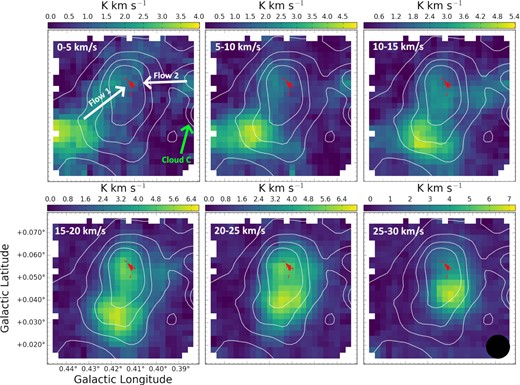
Mopra 22-m telescope data of HNCO emission towards cloud ‘d’ as part of the MALT90 Survey. The angular resolution of this data is 40 arcsec. Red contours show the 0.13 arcsec ALMA data presented in this paper. Black contours show BGPS data. The black circle in the bottom right plot represents the primary beam of the Mopra data. The data show channel maps of HNCO in the velocity range of 0−30 km s−1. Part of cloud ‘c’ is visible to the right of each map. At low velocities, the HNCO emission is found to the right and bottom left of the continuum emission peak (outlined by the ALMA contours). As the velocity increases, the emission from the right and bottom left both steadily move towards the continuum peak. The convergence of this velocity gradient at the location of the continuum peak is the same kinematic signature found by Henshaw et al. (2016a) in the gas upstream from the dust ridge. We interpret this kinematic structure as the convergence of pc-scale gas flows at the continuum peak of cloud ‘d’.
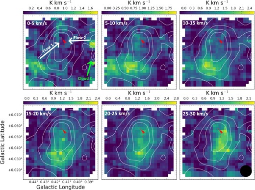
Mopra 22-m telescope SiO(2–1) data of cloud ‘d’ as part of the MALT90 Survey. The angular resolution of this data is 40 arcsec. Red contours show our 0.13 arcsec ALMA data and black contours show BGPS data. The black circle in the bottom right plot represents the synthesized beam. The data show channel maps of SiO in the velocity range 0 - 30 kms−1. Part of cloud ‘c’ is visible to the right of each map. A clear velocity gradient can be seen, with a point of convergence between clouds ‘d’ and ‘c’ at the point of our ALMA data.
The following interpretation of the three-dimensional motion assumes that the velocity along the line of sight is comparable to the velocity in the plane of the sky. At low velocities of 0−10 km−1, the HNCO and SiO emission is found to the right and bottom left of the continuum emission peak (outlined by the ALMA continuum contours). As the velocity increases, the emission from the right and bottom left both steadily move towards the continuum peak, converging at this location at a velocity of ∼20−25 km s−1.
In addition to these large-scale Mopra channel maps, we produce channel maps of the ALMA data. Figs 11 and 12 show the H2CO (30, 3–20, 2) and SiO (5–4) emission, respectively, at velocities in the range of 5−30 km s−1. The spatial morphology of the H2CO emission is dominated by two partially filled circular structures which intersect at the location of the dust continuum emission at a velocity of 15−20 km s−1. The SiO emission also shows a similar morphology, although less of both circles are filled, possibly due to the lower signal-to-noise ratio of the detection. A key difference between the SiO and H2CO morphologies is that the emission from the two overlapping H2CO circles coincides exactly with the dust emission, while the location of the overlapping circles in the SiO emission is offset to the right of the dust emission. Indeed, the SiO emission appears to be ‘wrapping around’ the right-hand edge of the dust continuum emission. This spatial offset is consistently equivalent to ∼7 beam widths, so must be real and not an observational artefact. No signs of SiO bipolar outflows indicative of ongoing star formation are detected.

A channel map of H2CO (30, 3–20, 2) from our ALMA data in the range of 5–30 kms−1. Black contours show the dust continuum emission of our ALMA data and green contours show SMA 1.3mm continuum data. The black circle in each plot represents the synthesised beam. Magenta dashed lines show the ‘hollow circle’ features described in Section 4.3. The velocity gradient in cloud ‘d’ observed on larger scales can also be seen on this smaller scale.
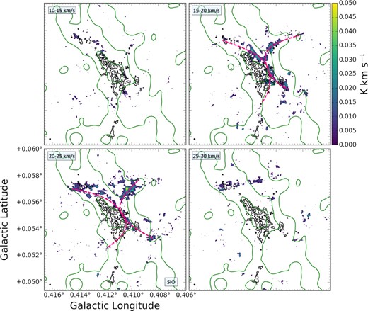
A channel map of SiO from our ALMA data in the range of 10−30 km s−1. Black contours show the dust continuum of our ALMA data and green contours show SMA 1.3 mm continuum data. The black circle in each plot represents the synthesized beam. Magenta dashed lines show the ‘hollow circle’ features described in Section 4.3. The velocity gradient seen on larger scales in cloud ‘d’ can be seen on this smaller scale.
We now try to interpret this information in a self-consistent way. The convergence of the large-scale HNCO and SiO velocity gradients at the location of the continuum peak is similar to the kinematic signature found in similar Mopra data by Henshaw et al. (2016c) in the gas upstream from the dust ridge. They showed that this velocity structure can arise from the convergence of large-scale gas flows due to global gravitational collapse. A natural interpretation of the HNCO and SiO kinematic structure in the Mopra data towards cloud ‘d’ is therefore that it is showing convergence of pc-scale gas flows at the continuum peak.
In this scenario, the curved ALMA dust continuum structure (at clump ‘d6’) is the most likely convergent point of the flows, with mass converging from across the entirety of cloud ‘d’. Given that the relative motion of the gas flows is highly supersonic, they should produce strong shocks at the intersection point. The fact that the SiO emission curves around the right-hand edge of the dust continuum emission provides strong evidence that there is a shock front at this location at VLSR = 15−20 km s−1.
As the ambient gas in the flows is already at high density, it should cool quickly after the shock front has passed, making this an isothermal shock. The post-shock density will therefore be enhanced by a factor |$\cal {M}^2$|, where |$\cal {M}$| is the Mach number of the shock (Padoan & Nordlund 2011). However, it is possible that C-shocks are present, and so the compression is not necessarily given by |$\cal {M}^2$|. The exact density enhancement will depend on the details of the shock. It is plausible that the gas traced by the ALMA dust continuum emission reached its high density through this process.
Here, the two unfilled circles in the ALMA H2CO channel maps represent the excitation- and density-enhanced gas along the intersection point of the two flows that converge at 15−20 km s−1 at the location of the dust continuum emission. The offset of the SiO emission to the right-hand side of the dust continuum emission shows the current location of the shock front. The curvature and central peak of the dust emission and the gas is strikingly similar to the bow shock morphology seen ubiquitously towards shocked regions.
To further illustrate the velocity flows we compute position–velocity (pv) diagrams of the two main flows in the HNCO Mopra data (Fig. 13). The diagrams were computed using the impv task within casa. The left-hand diagram was computed with a width of 5 pixels and the right-hand diagram was computed with a width of 1 pixel. While the velocity offset is more subtle in the right-hand flow, there is still a definite offset, converging with that of the much more obvious left-hand flow.
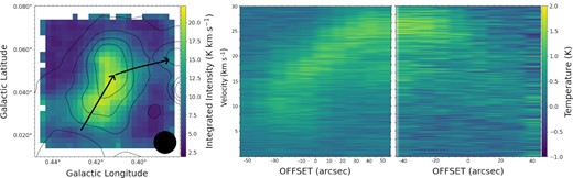
Left: Integrated intensity map of the Mopra HNCO line. Black arrows show the slices that the pv diagrams were computed across. Middle and right: Position–velocity (pv) diagrams of the two flows within the Mopra HNCO line.
In summary, all of the data to hand can be described as the result of a shock at the convergence point of two large-scale gas flows.
If this interpretation is correct, we estimate the time, t, it will take for all of the mass to end up at the convergence point through t = d/v, where v is the velocity of the gas and d is the distance the gas will travel. We use the earlier velocity dispersion of clump ‘d6’ of ∼2.1 kms−1 from Walker et al. (2018). We also use the effective radius of clump ‘d6’ of 0.16 pc from Walker et al. (2018) and double it to account for the gas moving across the entire clump. In this way, we estimate that it will take ∼105 yr for all the mass to reach the convergent point across clump ‘d6’. However, clump ‘d6’ is only a small part of cloud ‘d’, and so we must consider the whole cloud. From Walker et al. (2015), cloud ‘d’ has a radius of 3.2 pc and line widths of ∼ 16 km s−1, and so we estimate that all mass will converge across the entirety of cloud ‘d’ in around 3 × 10⁵ yr.
We estimate the corresponding mass inflow rate, |$\dot{m}$|, through, |$\dot{m} = m/t$|, where m is the gas mass. Using the upper mass limit of clump ‘d6’ of 239 M⊙ from Walker et al. (2018), we estimate a mass inflow rate towards the convergent point of the clump of 10−3 M⊙ yr−1. Once again considering the whole cloud, using the mass of 7.6 × 10⁴ M⊙ from Walker et al. (2015), we estimate a mass inflow rate across the entire cloud of around 0.25 M⊙ yr−1.
These estimates are all under the assumption that the material is all sitting in the same plane of the sky. However, there could be an offset along the line of sight, which would imply rotation, such as those in the simulations of Kruijssen et al. (2019b). This is because we are assuming that all of the gas is converging on one point. However, we do not know the 3D motions of the cloud. If they do not converge on this point, there could be net rotations in the gas. This may still lead to a collapse, but the process would be delayed when compared to collapse purely via convergence.
We conclude that a be funnelled towards the convergent point in a very short period of time (although this process may be delayed if there is an offset along the line of sight). This would quickly push the gas above the critical density threshold for star formation in the CMZ (Walker et al. 2018) and star formation will begin. This scenario would be in agreement with the results of Barnes et al. (2019), such that the gas would become bound and undergo collapse following the collision of both flows. In summary, it appears that star formation is imminent in cloud ‘d’ and that we have therefore identified a truly pre-star-forming YMC precursor gas cloud.
Source of converging flows
We now seek to understand the origin of these converging gas flows. As previously discussed, SiO emission is seen to be ‘wrapping around’ the right-hand edge of the dust continuum emission. The density required to excite the SiO (5–4) line across such a broad filament, coupled with the lack of SiO emission in the densest region, implies that a large-scale shock feature is present. Three plausible mechanisms that could drive large-scale gas flows and generate such a shock are gravitational collapse, a cloud–cloud collision, or a shock triggered by pericenter passage with the bottom of the gravitational potential.
Cloud–cloud collisions (CCCs) – collisions of molecular gas clouds (Hasegawa et al. 1994) – have been postulated as an explanation for various observed properties in multiple Galactic Centre clouds. These clouds include the ‘Brick’ (Higuchi et al. 2014; Johnston et al. 2014) and the 50 kms−1 cloud (Tsuboi, Miyazaki & Uehara 2015). There are many features that are attributed to CCCs. These features include shells or cavities (Higuchi et al. 2014; Tsuboi et al. 2015), multiple velocity components connected by ‘bridge features’ (Johnston et al. 2014; Tsuboi et al. 2021), and emission from shocked gas (Armijos-Abendaño et al. 2020; Zeng et al. 2020). Features that are unambiguously a signature of a CCC, however, are rare, particularly in an environment so complex as the CMZ. They may also occur at a much lower rate compared to other mechanisms that dominate the cloud lifetime (Jeffreson et al. 2018). Some shocks within the CMZ are caused by bar-driven streams colliding with clouds (Sormani, Binney & Magorrian 2015; Sormani & Barnes 2019; Hatchfield et al. 2021). Hatchfield et al. (2021) find that simulated CMZ clouds have peaks in their average density at the point where they collide violently with inflowing material. However, it is unlikely that the collision observed in cloud ‘d’ is driven by bar inflow, as cloud ‘d’ is not located near any proposed entry point to the CMZ (Henshaw et al. 2022a). It is also extremely unlikely that cloud ‘d’ is a collision occurring downstream from an entry point, as the collision is currently ongoing. However, the shocks at cloud ‘d’ could be the result of a collision between clouds independent of bar inflow.
Another possibility is that the shock has been caused by tidal forces in the clouds during their pericentre passage of the Galactic Centre. Hydrodynamic simulations performed by Dale, Kruijssen & Longmore (2019b) show that inclusion of tidal forces is required in modelling star formation in the centre of galaxies, and that the tidal forces experienced during pericentre passage temporarily increase the star formation rate by a factor of up to 2.7. It is possible that the shock in cloud ‘d’ is observational evidence of the tidal deformation found in the numerical simulations by Dale et al. (2019b).
While these scenarios, along with pure gravitational collapse, are all possibilities for the shock we see in cloud ‘d’, further work is required to unambiguously distinguish between them.
5 CONCLUSIONS
We report high-resolution (0.13 arcsec, 1000 au) ALMA Band 6 (1.3 mm, 230 GHz) observations towards the single-dish continuum peak of the Galactic Centre dust ridge cloud G0.412 + 0.052, also known as cloud ‘d’. We summarize the main results as follows:
This region of cloud ‘d’ contains substructures separated on 104 au scales. Using dendrograms to characterize the continuum structure, we identify 96 individual leaves above the 3σ level. The range in mass from 0.21 to 3.1 M⊙ has radii of ∼103 au and densities of 106−7 cm−3. Above the 5σ level, we identify nine leaves, with masses of 0.49−1.8 M⊙ and similar radius and density ranges.
The projected spatial separations of the continuum sources lie between the upper thermal Jeans length prediction and the lower turbulent Jeans length prediction. It is not clear which of these scales is favoured by the separation of the continuum sources, although there is a slight tendency towards thermal. However, the masses of the sources are consistent with thermal Jeans mass predictions but not turbulent Jeans mass predictions.
The mass distribution of compact continuum sources is bottom-heavy (mean mass ∼0.7 M⊙), and does not resemble a typical stellar initial mass function or pre-stellar core mass function. Stars forming from these initial sources would produce an extremely bottom-heavy IMF. Conversely, in order to populate a normal IMF, the initial sources will have to accrete many times their current mass from the surrounding environment to form the expected large number of intermediate and high-mass stars. We expect this cloud to form many high-mass stars, but find no high-mass starless cores.
None of the identified continuum sources coincide with known star formation tracers. In particular, we do not detect any molecular outflows via SiO (5–4) or 13CO (2–1) emission, nor do we detect any typical hot core tracers such as CH3CN. As star formation has been detected in similar CMZ cloud using an identical observational set-up, we conclude that cloud ‘d’ is not forming stars currently.
Virial analysis suggests that the continuum sources are most likely not gravitationally bound. However, they are subject to external pressures two to three orders of magnitude greater than those found in the Galactic disc. There is either an additional confining pressure on ∼1000 au scales that is undetected on the scale of clouds, or the sources are overpressured with respect to the surrounding gas and are therefore transient.
We find evidence from single-dish molecular line observations that suggest that cloud ‘d’ is a point of convergence of larger scale gas flows. It is estimated that all mass will have converged on this point in ∼105 yr at a mass inflow rate of ∼10−3 M⊙ yr−1. If the cloud continues to collapse and the sources continue to grow via accretion of this material, then the cloud has the potential to begin forming stars in this time frame, although we cannot confirm the mechanism by which they will form.
We conclude that cloud ‘d’ is the earliest known pre-star forming massive cluster and therefore is an ideal laboratory in which to study the initial conditions of star and cluster formation in extreme environments. These initial conditions shape the IMF and set global star-forming relations in extreme (but cosmologically typical) conditions and therefore further study of cloud ‘d’ and its counterparts is important to further our understanding.
SUPPORTING INFORMATION
Table A1. Masses, radii, and number densities (assuming spherical geometry) of each the 96 individual potential star-forming sources we have detected using dendrogram analysis, as well as estimated masses and number densities with background emission subtracted.
Please note: Oxford University Press is not responsible for the content or functionality of any supporting materials supplied by the authors. Any queries (other than missing material) should be directed to the corresponding author for the article.
ACKNOWLEDGEMENTS
This paper makes use of the following ALMA data: ADS/JAO.ALMA#2016.1.00949.S. ALMA is a partnership of ESO (representing its member states), NSF (USA) and NINS (Japan), together with NRC (Canada), MOST and ASIAA (Taiwan), and KASI (Republic of Korea), in cooperation with the Republic of Chile. The Joint ALMA Observatory is operated by ESO, AUI/NRAO and NAOJ. BAW thanks Matt, Luke, and Ash for their continued support and encouragement, and acknowledges an STFC doctoral studentship. DLW and CB acknowledge support from the National Science Foundation under Award No. 1816715 and CB also acknowledges support under Award No. 2108938. ATB would like to acknowledge funding from the European Research Council (ERC) under the European Union’s Horizon 2020 research and innovation programme (grant agreement no. 726384/Empire). GG acknowledges support from ANID project FB210003. LCH was supported by the National Science Foundation of China (11721303, 11991052) and the National Key R&D Program of China (2016YFA0400702). JMDK and MAP gratefully acknowledge funding from the European Research Council (ERC) under the European Union’s Horizon 2020 research and innovation programme via the ERC Starting Grant MUSTANG (grant agreement number 714907). JMDK gratefully acknowledges funding from the Deutsche Forschungsgemeinschaft (DFG) in the form of an Emmy Noether Research Group (grant number KR4801/1-1). XL was supported by JSPS KAKENHI grant no. 20K14528.
DATA AVAILABILITY
The data products used to conduct the research presented in this paper are made publicly available at the following Zenodo repository: https://doi.org/10.5281/zenodo.6546462. Scripts used to conduct this research are also made available on GitHub at: https://github.com/b-a-williams/Cloud-d-ALMA.
REFERENCES
APPENDIX
See Table A1.
This is a sample table, the full table is available online as supplementary material. Masses, radii, and number densities (assuming spherical geometry) of each the 96 individual potential star-forming sources we have detected using dendrogram analysis, as well as estimated masses and number densities with background emission subtracted.
| Right | Background | Background | |||||
|---|---|---|---|---|---|---|---|
| Source number | ascension | Declination | Mass | Radius | n | subtracted mass | subtracted n |
| (deg) | (deg) | (M⊙) | (103 au) | (106 cm−3) | (M⊙) | (106 cm−3) | |
| 1 | 266.5949552 | −28.56055698 | 0.71 | 1.71 | 6.04 | 0.06 | 0.54 |
| 2 | 266.5950498 | −28.56040786 | 2.82 | 3.31 | 3.3 | 0.39 | 0.45 |
| 3 | 266.5921428 | −28.56046861 | 0.92 | 1.96 | 5.21 | 0.23 | 1.28 |
| 4 | 266.5954069 | −28.56032063 | 1.00 | 2.02 | 5.14 | 0.22 | 1.14 |
| 5 | 266.5947927 | −28.56023752 | 0.48 | 1.42 | 7.06 | 0.05 | 0.69 |
| 6 | 266.5949923 | −28.56017972 | 0.25 | 1.04 | 9.42 | 0.04 | 1.32 |
| 7 | 266.5948637 | −28.56005386 | 0.76 | 1.78 | 5.67 | 0.08 | 0.62 |
| 8 | 266.5947918 | −28.55997624 | 0.4 | 1.31 | 7.57 | 0.05 | 0.95 |
| 9 | 266.594819 | −28.55975369 | 0.35 | 1.3 | 6.7 | 0.04 | 0.78 |
| 10 | 266.5947906 | −28.55961351 | 0.37 | 1.33 | 6.61 | 0.04 | 0.81 |
