


ABSTRACT
We present the results of an investigation of the giant radio pulse (GRP) generation rate from five radio pulsars (B0301+19, B0950+08, B1112+50, B1133+16, and B1237+25) and anomalous intensity pulse generation rate from B0809+74. All data used were obtained with the Large Phased Array radio telescope at the Pushchino Radio Astronomy Observatory at 111 MHz from 2012 to 2021. In addition to the analysis of the rate of generation of bright pulses, we analyse the distribution of bright pulses in the phase of the pulsar period and search for clusters of bright pulses – several bright pulses emitted in adjacent pulsar periods. It is found that pulsars B0301+19, B1112+50, B1133+16, and B1237+25 demonstrate different generation rates and generation of clusters. Pulsar B1112+50 generates GRP clusters more often than the other pulsars studied. The longest cluster of GRPs containing four single pulses is detected from this pulsar. GRPs from the pulsars studied are distributed along the longitudes of the main components of the average pulses of these pulsars. This distribution is 1.5–2 times narrower than the phase distribution of non-giant pulses. It is found that the distance between the components of the average GRP profile and the distance between the components of the average non-giant profile differ substantially for pulsars with multicomponent average profiles.
1 INTRODUCTION
The large group of radio pulsars shows small pulse-to-pulse intensity variations within the limits of 10 times the intensity of the averaged pulse. However, some pulsars demonstrate unpredictable short-duration outbursts of pulsed radio emission. These pulses are known as giant radio pulses (GRPs).
At the present day, only about 16 pulsars are known to be GRP emitters (Staelin & Reifenstein 1968; Wolszczan, Cordes & Stinebring 1984; Singal 2001; Ershov & Kuzmin 2003; Johnston & Romani 2003; Joshi et al. 2004; Kuzmin & Ershov 2004; Knight et al. 2005; Ershov & Kuzmin 2005; Kuzmin & Ershov 2006; Crawford et al. 2013; Kazantsev & Potapov 2017; Kazantsev, Potapov & Safronov 2019), i.e. emit individual pulses that satisfy the GRP criteria (the peak flux densities of GRPs exceed the flux density in the average profile of a pulsar by a factor of 30). These pulsars can be divided into two groups: pulsars with strong magnetic fields at their light cylinders (over BLC > 105 gauss) and millisecond and ordinary pulsars with BLC from several to several hundred gauss. Well-known representatives of the former group are the Crab pulsar (Staelin & Reifenstein 1968) and the millisecond pulsar B1937+21 (Wolszczan et al. 1984). There are a lot of theoretical models concerning GRPs from bright fast-rotating pulsars of the first group (Hankins et al. 2003; Istomin 2004; Petrova 2006; Machabeli, Chkheidze & Malov 2019), but much less is known about pulses from ordinary pulsars with GRPs.
Still, we consider that studies of GRPs from radio pulsars are equally important for understanding the pulse generation mechanism. In our earlier work (Kazantsev & Potapov 2018), we analysed the energy characteristics of this group of pulsars. However, we have not studied the temporal properties of GRP generation. This issue is clearly very important, because it can shed light on the dynamical behaviour of the GRP generation mechanism.
Here we present a statistical study of the rate of GRP emission from six pulsars: B0301+19, B0809+74, B0950+08, B1112+50, B1133+16, and B1237+25. All the listed pulsars have been previously noted as generators of sporadic bright individual pulses, mainly at low frequencies. A detailed study of the GRPs of the pulsar B0301+19 was carried out in Kazantsev et al. (2019). In this investigation, an analysis of 257 observation sessions at 111 MHz was performed, and it was shown that 2.5 per cent of the individual pulses of the pulsar exceed the peak flux density in the average profile by a factor of 30. The distribution of the individual pulses of this pulsar has a complex shape, with a pronounced power-law tail formed by bright individual pulses. Ulyanov et al. (2006) found very bright pulses 50–100 times higher than the average profile in amplitude from the pulsar B0809+74. The authors call these pulses ‘anomalous intensity pulses’; for this reason we use this term to describe bright pulses from the pulsar B0809+74. The emission of pulses of anomalous intensity can be similar to the GRP emission, and the long-term analysis of these pulses can be very useful for understanding the nature of their generation. Giant pulses from the pulsar B0950+08 were detected at 103 MHz by Singal (2001). The authors analysed about 1 million individual pulsar pulses received with the Rajkot radio telescope and showed that about 1 per cent of these pulses exceed the average pulsar profile by more than 100 times. An analysis of the distribution of pulses by the peak flux density, however, was not carried out in that investigation. Later, in Cairns, Johnston & Das (2004), it was discovered that there are several components of radiation from B0950+08: GRP emission, emission of giant micropulses, and several others. All these components have a power law of energy distribution and differ in their power-law indices. The lack of similar investigations for other pulsars with GRPs, such as B0031−07, B0301+19, B1133+16, etc., does not allow us to assert unambiguously that these emissions are characteristic only of the pulsar B0950+08. At the same time, it is impossible to unambiguously distinguish giant pulses and several merged giant micropulses from each other in observations of pulsars with emissions similar to that of B0950+08 at low frequencies and with insufficient time resolution. Such an analysis requires observations at high frequencies, as was done in Cairns et al. (2004). The analysis of powerful individual pulses from B0950+08 was carried out at low frequencies in Singal & Vats (2012) and Smirnova (2012) and it was shown that the aggregate statistics of these emissions unambiguously illustrates this pulsar as a pulsar with GRPs, which makes it possible to include it in our sample. GRPs from the pulsar B1112+50 were discovered by Ershov & Kuzmin (2003). The authors analysed 172 observation sessions and found 126 GRPs (on average 1 GRP per 150 pulsar periods), exceeding the flux in the average profile by a factor of 30. The authors also noted the generation of GRPs from this pulsar in pairs and triplets, and estimated the period of pulsar activity at several seconds. The authors pointed out the presence of a pronounced power-law tail in the distribution of pulses over the peak flux density, which corresponds to bright individual pulses of the pulsar. Kramer et al. (2003) reported bright pulses from B1133+16 at 5 GHz. In Karuppusamy, Stappers & Serylak (2010) it was shown that the pulsar B1133+16 emits bright pulses in the range 110–180 MHz. These pulses are 10 times higher than the average pulsar profile in amplitude, and the distribution of individual pulses over peak flux densities is a power law. Similar results were obtained in this work for the pulsar B1112+50, which is also included in our sample. A more detailed analysis of GRPs from B1237+25 was done by Kazantsev & Potapov (2017). The pulsar regularly emits pulses with a high flux density in comparison with regular pulses, constant localization at the longitude of one of the components of the average profile, which is from 50 to 100 per cent of the duration of the corresponding component. The distribution of individual pulses over the peak flux density is well approximated by a power law.
It is important to note once again that not all of the pulsars listed above are noted in the literature as sources of GRPs. In addition, several of these pulsars have their own peculiarities in generating bright pulses (for example, B0950+08). Analysis of flare activity over long periods for a given sample of active pulsars can provide the necessary material to search for similarities and differences in the mechanisms of emission of bright individual pulses of these pulsars.
This article is structured as follows: in Section 2 we describe the process of obtaining data and the methods of data analysis; Section 3 contains the results of the analysis for each pulsar. Discussions and our conclusions are presented in Sections 4 and 5, respectively.
2 OBSERVATIONS AND DATA PROCESSING
Our observations were made with the Large Phased Array transit radio telescope of the Pushchino Radio Astronomy Observatory (LPA LPI) at the Astro Space Center, P. N. Lebedev Physical Institute. This is a low-frequency radio telescope with a central frequency equal to 111 MHz and an effective bandwidth equal to 2.3 MHz. During our observational sessions, the telescope effective area was 20 000 ± 1300 m2 in the zenith direction. Single linear polarization was used.We used a sampling interval of 1.2288 ms for all observational sessions. The LPA LPI observes pulsars during their culmination only, when they cross the beam of the LPA LPI. As a result, the duration of observations depends on the declination of a pulsar. For example, the duration of a single observational session of B0809+74 is equal to ∼11 min; that of B1237+25 to ∼3.5 min.
Our data-processing pipeline can be described as follows. The digital receiver gets the phased analogue signal from the radio telescope. After that, using the synchronizer that generates trigger pulses, the signal is split into a sequence of segments with a duration equal to the period of a given pulsar. The synchronizer has ±100 ns accuracy when converting GPS time to the universal time-scale and ±10 ns accuracy when setting the start time of the receiver. These levels of accuracy are sufficient for observing normal-period pulsars at the central frequency of LPA LPI and performing phase analysis of individual pulses from these pulsars.
The signal is digitized at a frequency of 5 MHz for each pulse. The digitized pulse is accumulated in the receiver’s buffer. After digitization, all readings for a given pulsar are loaded into the fast Fourier transform hardware processor from the buffer. The processor returns the digitized signal as a raw-file observation. The file consists of a header with common information (name of pulsar, start time of observation, time sample, etc.) and an array of time-series spectra. The data for the time-series spectra are recorded as 32-bit floating-point numbers. This algorithm does not include absolute calibration of intensity, and units of intensity are analogue-to-digital converter (ADC) units. The next stage of data processing is the offline de-dispersion procedure (Hankins & Rickett 1975), which is done at a fixed dispersion measure (DM) for a given pulsar (see Table 1). The de-dispersed pulses for a given observation are saved for a subsequent analysis. The de-dispersed individual pulses of a pulsar recorded in an observing session are summed up synchronously with the pulsar period to form a dynamic average pulse (average pulse per one observing session). The individual pulse is considered to be a GRP if its peak flux density exceeds that of the dynamic average pulse by 30 times or more. We used a similar criterion for identifying GRPs in our early studies of these pulsars (e.g. Kazantsev & Potapov 2017, 2018; Kazantsev et al. 2019). This makes it possible to use the GRP statistics obtained in this and the above-mentioned works in further investigations. The selection of GRPs in amplitude relative to the average profile of a pulsar has been used in the studies by other authors (e.g. Ershov & Kuzmin 2003; Kuzmin & Ershov 2004; Smirnova 2012; Singal & Vats 2012; Tsai et al. 2015). However, for an extraction of radio giant pulses the intensity distribution of individual pulses also needs to be taken into account since they have been observed to be power-law distributed (Staelin & Reifenstein 1968). The corresponding distributions of individual pulses for the studied sample are given in Fig. 1. The Freedman–Diaconis rule (Freedman & Diaconis 1981) was used to define the width of the bins that were used in the distributions. A non-linear least-squares method was used to fit the distributions. It is important to note that the use of the dynamic average profile as a giant/non-giant separator provides information on the modulation of radiation within a single observation session.
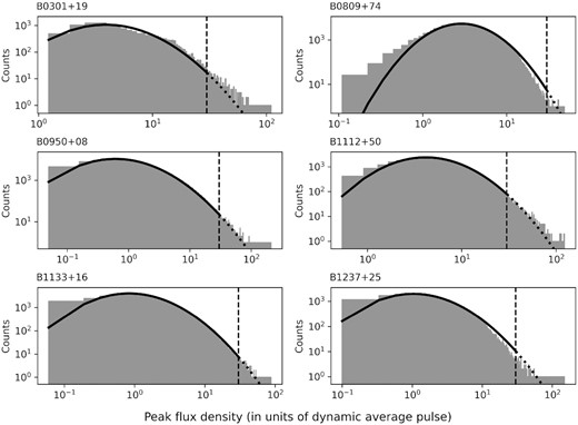
Distribution of individual pulses by peak flux density in units of the dynamic average profile for each of the pulsars studied. The solid and dotted lines show the fitting of the distribution by the lognormal function. The vertical dashed line shows the cutoff level of 30 dynamic average profiles of the pulsar.
Parameters of pulsars and durations of the observations of each pulsar.
| Pulsar name | RA | Dec. | P | dP/dt | DM | PEpoch | Years | Sessions | Total observational time |
|---|---|---|---|---|---|---|---|---|---|
| (epoch 1950) | (J2000) | (J2000) | (s) | (10−15 s s−1) | (cm−3 pc) | (MJD) | (h) | ||
| B0301+19 | 03h04m33|${_{.}^{\rm s}}$|115 | 19°32′51|${_{.}^{\prime\prime}}$|4 | 1.3876 | 1.29 | 15.66 | 49289.00 | 2012–2021 | 752 | 42.32 |
| B0809+74 | 08h14m59|${_{.}^{\rm s}}$|50 | 74°29′05|${_{.}^{\prime\prime}}$|70 | 1.2922 | 0.17 | 5.75 | 49162.00 | 2012–2020 | 534 | 106.03 |
| B0950+08 | 09h53m9|${_{.}^{\rm s}}$|3097 | 07°55′35|${_{.}^{\prime\prime}}$|75 | 0.2531 | 0.23 | 2.97 | 46375.00 | 2012–2021 | 1179 | 63.4 |
| B1112+50 | 11h15m38|${_{.}^{\rm s}}$|400 | 50°30′12|${_{.}^{\prime\prime}}$|29 | 1.6564 | 2.49 | 9.19 | 49334.00 | 2012–2020 | 1540 | 128.25 |
| B1133+16 | 11h36m3|${_{.}^{\rm s}}$|1198 | 15°51′14|${_{.}^{\prime\prime}}$|183 | 1.1879 | 3.73 | 4.84 | 46407.00 | 2013–2020 | 1050 | 56.11 |
| B1237+25 | 12h39m40|${_{.}^{\rm s}}$|4614 | 24°53′49|${_{.}^{\prime\prime}}$|29 | 1.3824 | 0.10 | 9.25 | 46531.00 | 2012–2021 | 781 | 45.77 |
The following parameters were calculated for each detected GRP:
Time stamp of the first sample (MJD),
Time of arrival (MJD),
Amplitude of GRP (ADC units),
STD noise (ADC units),
Width of pulse at 50 per cent of peak (ms),
Width of pulse at 10 per cent of peak (ms).
The rate of GRP generation were calculated in 30 d bins and normalized to the total duration of observations in the corresponding bins. Taking into account the time-scale of the nine-year observation, this bin size is optimal, since it allows us to detect variations on scales from months to years. Additionally, a search for clusters of GRPs is performed. A cluster means a sequence of giant pulses emitted in adjacent periods.
A method of control charts, also known as Shewhart charts (Shewhart 1930), were chosen to determine the stability of the rate of GRPs, namely, individuals and moving-range (XmR) charts. The individuals chart displays the individual measured values. The moving-range chart displays the difference from one point to the next. These charts show changes in processes or phenomena that change the mean or variance of the measured statistic. The statistical criterion of instability in these charts is the excess of the mean |$\bar{x}$| by three standard deviations σ. We call the level |$\bar{x}+3\sigma$| the upper control limit (UCL) and the level |$\bar{x}-3\sigma$| the lower control limit (LCL).
3 RESULTS
The resultant statistical properties of the rate of GRP generation are presented in Table 2. We present information about clustered GRPs separately in Table 3. Below, detailed information about each pulsar is provided.
XmR chart parameters.
| Parameters | B0301 | B0809 | B0950 | B1112 | B1133 | B1237 |
|---|---|---|---|---|---|---|
| Mean(x) | 0.12 | 0.01 | 0.44 | 0.26 | 0.07 | 0.06 |
| UCL(x) | 0.45 | 0.03 | 1.18 | 0.47 | 0.28 | 0.33 |
| LCL(x) | −0.21 | −0.02 | −0.31 | 0.05 | −0.14 | −0.20 |
| Mean(MR) | 0.09 | 0.01 | 0.20 | 0.08 | 0.06 | 0.07 |
| UCL(MR) | 0.34 | 0.03 | 0.77 | 0.28 | 0.23 | 0.33 |
Notes. Mean(x) is the measured process centre.
UCL(x) is the +3σ upper control limit.
LCL(x) is the −3σ lower control limit.
Mean(MR) is the measured moving-range centre.
UCL(MR) is the +3σ upper control limit of the moving range.
Clusters of GRPs. Numbers of detected pairs of GRPs are in the second column, number of instances of clusters with >2 GRPs are in the third column, and in the last column we show the maximal size of the cluster for each pulsar.
| Name | 2 GRPs | >2 GRPs | Max size of cluster |
|---|---|---|---|
| B0301+19 | 6 | 1 | 3 |
| B0809+74 | 1 | 0 | 2 |
| B0950+08 | 50 | 6 | 3 |
| B1112+50 | 75 | 5 | 4 |
| B1133+16 | 1 | 0 | 2 |
| B1237+25 | 1 | 0 | 2 |
| Name | 2 GRPs | >2 GRPs | Max size of cluster |
|---|---|---|---|
| B0301+19 | 6 | 1 | 3 |
| B0809+74 | 1 | 0 | 2 |
| B0950+08 | 50 | 6 | 3 |
| B1112+50 | 75 | 5 | 4 |
| B1133+16 | 1 | 0 | 2 |
| B1237+25 | 1 | 0 | 2 |
3.1 PSR B0301+19
During the processing of 752 observation sessions of the pulsar B0301+19, 14 588 individual pulses were detected with a signal-to-noise ratio (SNR) of more than four; out of these, 322 individual pulses were identified as GRPs according to our selection criterion. This pulsar demonstrated quite an unstable rate of GRP generation, since strong modulation is noticeable (see Fig. 2, B0301+19). The average rate is about eight giant pulses per hour. There is a jump in the rate of GRP generation around the MJD 58634 epoch. The maximal rate reaches a value of 31 GRPs per hour. For a significant number of sessions, no individual pulses that could be classified as GRPs were detected.
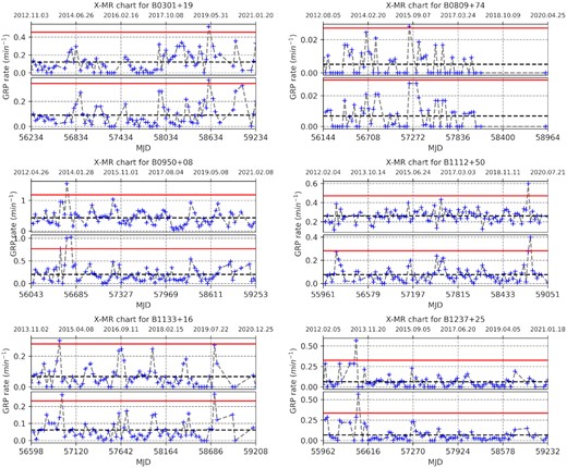
Individuals (upper panels) and moving-range (lower panels) charts of GRPs of the pulsars studied. Each point contains data averaged over 30 d.
In the framework of a search for GRP clusters, six clusters from B0301+19 were detected. The longest cluster includes three successively emitted GRPs of the pulsar (Fig. 3).
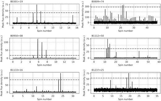
Examples of GRP clusters. The grey dashed line shows the GRP threshold; i.e. flux density is 30 times larger than the peak flux density of the dynamic averaged pulse.
The phase distribution of individual pulses from B0301+19 is shown in Fig. 4. The giant pulses of the pulsar are located along the longitudes of the main components of the average pulse. Out of all the registered GRPs, 124 are localized on the first component of the average profile, and 192 are localized on the second component.
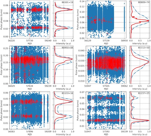
Left: Phase distribution of non-giant (blue points) and giant (red points) pulses from the pulsars studied. Right: the averaged GRP (red solid line) and the non-giant averaged pulse (blue dashed line) for the pulsars studied.
The fitting of the averaged GRP and average pulse, which includes all registered non-giant pulses, is shown in Fig. 5. According to the fitting results, the distance between the components of the average pulse is (66.1 ± 0.2) ms. The same parameter for the averaged GRP is equal to (64.6 ± 0.2) ms. In units of the pulsar period, these distances are 0.0477 and 0.0465, respectively.
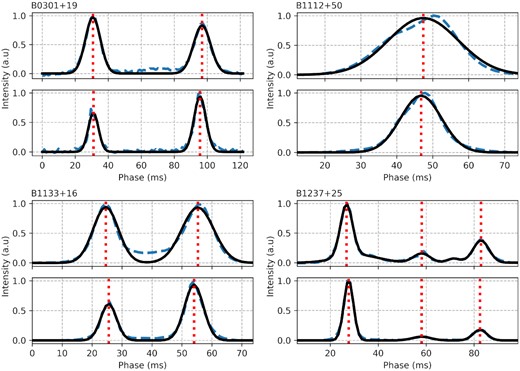
Fitting results for averaged pulses (upper panels) and the averaged GRPs (lower panels) for several studied pulsars. Blue dashed lines show an averaged pulse and an averaged GRP for each pulsar. Black solid lines show the corresponding fitting by a combination of Gaussian functions. Red dotted lines show the location of the peak for the corresponding Gaussian function.
3.2 PSR B0809+74
In 534 observations of PSB B0809+74, 261 108 pulses with SNR > 4σ were detected. As we have already mentioned, this pulsar is usually not considered to be a GRP emitter. Nevertheless, it sometimes generates individual pulses that exceed the amplitude of the average profile by 30 or more times (Ulyanov et al. 2006). We detected 39 such pulses. The rate of anomalous intensity pulse generation was the lowest among the pulsars studied by absolute value (see Table 2). There were no strong individual pulses in most observation sessions (see Fig. 2, B0809+74). Nevertheless, there were sessions with an increased generation rate. On average, B0809+74 generates approximately one anomalous intensity pulse in 2 h of observations. The maximum detected rate of GRP generation was two pulses per hour.
We found only one cluster of two consecutive strong pulses (see Fig. 3).
Strong pulses are located in the middle of the longitude of the average pulse (see the left-hand panel of Fig. 4). In view of the small number of detected strong pulses, the average pulse is highly jagged (see the right-hand panel of Fig. 4).
3.3 PSR B0950+08
We analysed 313 227 individual pulses from B0950+08 whose peak flux exceeds 4σ. Out of these, 1688 were GRPs. Pulsar B0950+08 showed a sinusoidal variation in GRP generation rate with a period of about 300 d (see Fig. 2). There were only several ‘empty bins’, where no GRPs were registered. The rate of generation varies between 0.1 and 1 min−1 with the average value equalling 0.44 min−1 or 26 GRPs per hour. There is a jump in rate around epoch MJD 56500 where it increased by approximately 3.5 times, up to 93 GRP per hour.
We detected 50 clusters of GRPs from B0950+08. Six of these include three consecutive GRPs. An example of one of these groups is presented in Fig. 3.
The average pulse of pulsar B0950+08 is fairly complex (see the right-hand panel of Fig. 4). It includes a precursor area (0–0.12 pulse phase) and a main pulse (0.12–0.25 pulse phase). 92 per cent of the GRPs are on the main pulse longitudes. Most frequently, GRPs were generated at the phase range of the second component of the main pulse of the pulsar. As a result, the shapes of the averaged GRP and average pulse are quite different. In addition, one can see GRP activity in the precursor area. It is clearly seen that near MJD 56430 and MJD 57232 the GRPs were actively emitted both in the precursor area and at the trailing edge of the main profile. Strong modulation activity at precursor longitudes has previously been noted (Cairns et al. 2004; Smirnova 2012).
3.4 PSR B1112+50
In 1540 observation sessions of B1112+50, 65 034 individual pulses were found with a signal-to-noise ratio of more than 4σ; of these, 2023 met the GRP criterion. The pulsar B1112+50 demonstrates a sufficiently stable rate of GRP generation (see Fig. 2). Nevertheless, a jump in the rate of generation can be seen around MJD 58740. At a maximum, the rate of GRP generation reaches 36 pulses per hour. Compared to the average, this gives about 16 giant pulses per hour.
Also, we detected the largest number of clusters from this pulsar, 75 (see Table 3). In five cases, the number of GRPs exceeds two and the largest cluster contained four pulses. In Fig. 3 we show one of the largest clusters.
The simple Gaussian-like shape of an average pulse is typical for the pulsar B1112+50. However, there is an asymmetry in the averaged pulse shape (see the right-hand panel of Fig. 4). GRPs from B1112+50 were distributed randomly along the average pulse longitude, which was narrower than the distribution of non-giant pulses. The averaged GRP was about twice as narrow as the averaged pulse, which included all non-giant pulses from this pulsar. There was a significant offset between the peaks of the averaged GRP and average pulse. However, according to the fitting, the profile’s location is quite similar (see Fig. 5). For the averaged GRP, the mean of the Gaussian form is equal to (46.76 ± 0.06) ms; for the average non-giant profile it is equal to (47.38 ± 0.15) ms. In units of the pulsar period, these locations are 0.0282 and 0.0286, respectively.
3.5 PSR B1133+16
In the 1050 observation sessions analysed for this pulsar, 107 379 individual pulses with a signal-to-noise ratio of more than 4σ were detected. Out of these, 236 individual pulses were classified as GRPs. The rate of GRP generation of B1133+16 is visibly unstable (see Fig. 2, B1133+16). The maximum rate generation is 18 GRPs per hour. On average, the pulsar generates around four GRPs per hour, but for B0809+76 there were no detections in numerous sessions. B1133+16 generates only one cluster of GRPs, as shown in Fig. 3.
B1133+16 has a double-component average pulse (see the right-hand panel of Fig. 4). The distribution of non-giant pulses shows that these pulses could be recorded between the main components of the profile. In the great majority of cases, GRPs were detected on the longitudes of the main components only. 60 per cent of the registered GRPs were detected on the second component of the pulsar average profile. The fitting results show that the distance between the main components for the averaged GRP and the average pulse is significantly different (see Fig. 5, B1133+16). For the average pulse, the distance is equal to (30.7 ± 0.3) ms; for the averaged GRP it is equal to (28.49 ± 0.12) ms. In units of the pulsar period, these distances are 0.0259 and 0.0240, respectively.
3.6 PSR B1237+25
We analysed 37 483 individual pulses from B1237+25 with a signal-to-noise ratio of more than 4σ. Out of these, 145 were classified as GRPs. The pulsar B1237+25 shows a fairly stable GRP generation rate (see Fig. 2, B1237+25). GRPs were detected in 70 per cent of the observed sessions. On average, PSR B1237+25 generates approximately four GRPs per hour. The maximum value of the GRP rate is 34 giant pulses per hour. We detected only one cluster of GRPs (see Fig. 3, B1237+25). The average pulse of B1237+25 is very complex and includes five components. Only three components (1, 3, and 5) can be reliably identified in one observation session at low frequency. The sum of numerous individual pulses allowed us to detect all five components of the average pulse. As seen in Fig. 4, the GRPs are emitted on the longitudes of the 1, 3, and 5 components. In 77 per cent of cases, giant pulses are recorded in the first component of the average profile. The fifth component accounted for 19 per cent of detected giant pulses, the third 4 per cent. We used the sum of five Gaussian functions (see the upper panel of Fig. 5) for fitting the complex average pulse of B1237+25. As a result, the positions of the 1, 3, and 5 components for the average pulse are equal to (26.70 ± 0.04), (58.4 ± 0.20), and (82.94 ± 0.09) ms, respectively. The shape of the averaged GRP is from three components only, and we used the sum of three Gaussian functions to fit this profile (see the lower panel of Fig. 5). The locations of the components of the average GRP are (27.62 ± 0.02), (58.1 ± 0.5), and (82.44 ± 0.14) ms. In this case, the difference between the most distant components (1 and 5) for the average GRP and the average non-giant pulse is equal to (54.82 ± 0.16) and (56.24 ± 0.12) ms, respectively. In units of the pulsar period, these distances are 0.0397 and 0.0407.
4 DISCUSSION
The pulsars considered in this analysis (except B0809+74) are GRP emitters with small values of magnetic field on a light cylinder. Existing theoretical models of GRP generation (e.g. Hankins et al. 2003; Istomin 2004; Petrova 2006; Machabeli et al. 2019) have been basically aimed at explaining the power law of the distribution of bright pulses and the extremely short duration of the GRPs found in the pulsar B0531+21 (Hankins et al. 2003). Such parameters of GRP emission as generation rate or the duration of the period of activity were not considered in these works. However, it seems to us very reasonable to hypothesize that since all the mentioned models are based on the basic pulsar parameters (the period of rotation and its first derivative). According to these models, the GRP generation should be similar for pulsars with similar periods and period derivatives. Not only should the pulse distribution, polarization, and duration of the GRPs be similar, but also such parameters as the rate of generation of GRPs and the generation of clusters of GRPs should be too. We have obtained the opposite result. Pulsars with highly similar physical parameters (e.g. B1112+50, B1133+16, and B1237+25) differ in rate of generation of GRPs and generation of clusters of GRPs.
According to our observations and analysis, the rate of generation of GRPs from the pulsars studied varies significantly in the considered time interval. Each pulsar demonstrates at least one significant increase in the GRP generation rate (see Fig. 2).
One can interpret this finding in several ways. First, it may reflect the instability of the mechanism of GRP generation. However, the emission rate of typical individual pulses is also subject to strong variability. In this way, the detected rate of GRPs may reflect the common nature of pulsed emission, both giant and normal.
The rates of generation of pulsars B1112+50 and B0950+08 are peculiar because they remain at a sufficiently high level during the periods studied. We detected the largest number of clusters of GRPs from these pulsars in comparison with other ones. The difference cannot be explained by different durations of observations: although the total time of observation of the pulsar B1112+50 is around three times longer than the total time of observation of pulsars B1133+16 and B1237+25, the number of detected clusters is 75 times larger.
Another striking feature of B1112+50 is the longest sequence of GRPs. At period 1.6564 s (see Table 1) the duration of emission of this group of giant pulses is approximately seven seconds. This could mean that the process giving rise to GRPs in the magnetosphere of this pulsar is not burst-like, but extended in time. This is the only pulsar in our study that demonstrated such extraordinary behaviour.
The rates of GRP generation of the pulsars B1237+25 and B1133+16 are similar – they have almost the same value of the average rate: 0.06 and 0.07 min−1, respectively.
The analysis of phase distribution shows that GRPs are located on the longitudes of the main components of average profiles of pulsars. However, the variance in longitude for the GRPs is much smaller. Moreover, for pulsars with multicomponent average profiles, the distance between the components of the averaged profile produced using GRPs only is less than the same distance for the average profile that includes non-giant pulses. For B1133+16, the difference between the distances mentioned above is (2.2 ± 0.4) ms. Taking into account the model of the nested-cone structure (Rankin 1993; Gil, Kijak & Zycki 1993), this difference, as well as the narrow distribution of the GRPs over the longitudes of the components, quite likely indicates that the GRPs of these pulsars are generated closer to the surface of the neutron star. Analysis of the phase distribution of giant pulses of the pulsar B0531+21 (Bij et al. 2021) does not show a noticeable difference in the arrival times of strong and weak pulses.
Detected sinusoidal variations in the rate of B0950+08 GRPs cannot be associated with any distortions in the telescope (change in the effective area or change in the gain), since the GRP sampling criterion that we used takes into account factors associated with the telescope. Something similar is also observed from B1133+16. This behaviour of the generation rate can be most interesting when applied to the formation of GRPs as an energy-accumulation mechanism in pulsar magnetosphere plasmas (Machabeli et al. 2019). At the same time, the study of the rate of generation from MJD 57638 to MJD 58624 (Kuiack et al. 2020) has given estimates of 30 GRPs per hour, while our estimates indicate this value as the average value of the rate of generation for B0950+08.
In addition, the average profile of the pulsar B0809+74, which includes only the GRPs, strongly differs from the average profile of the non-giant pulses. In the distribution of the GRP phase (right-hand panel of Fig. 4, B0809+74), one can notice a clear drift in the position of the GRPs along the longitudes of the average profile. It is known that this pulsar has a pronounced drift of subpulses, first discovered by Page (1973) and further studied in detail by e.g. Backer, Rankin & Campbell (1975), Rankin, Ramachandran & Suleymanova (2006), and Rankin & Rosen (2014). Due to the lack of observations of this pulsar in 2018 and 2019, we cannot state with confidence that the systematic drift of the GRP generation region in the phase of the average profile is not accidental. Further observations of this pulsar will help to confirm or refute the feature that we have discovered.
5 CONCLUSIONS
An analysis of variations in the rate of generation of powerful individual pulses of six pulsars of the Northern hemisphere at 111 MHz on a time-scale of nine years is presented.
It is shown that pulsars B0301+19, B1112+50, B1133+16, and B1237+25, which have been noted as GRP generators and have similar physical parameters (rotation period, period derivative, and the magnetic field on the light cylinder), demonstrate different generation rates and cluster generation. Each of the pulsars studied demonstrates jumps in the rate of GRP generation by 2–4 times from the average level. In the pulsar B1237+25, the maximal generation rate was found to exceed 10 times the average level. In the overwhelming majority of observations, the value of the generation rate is below the corresponding upper control limit.
GRPs from these pulsars are distributed along the longitudes of the main components of an average pulse. This distribution is 1.5–2 times narrower than the phase distribution of non-giant pulses. A systematic shift in the position of the GRPs was found in the pulsar B0809+74.
For pulsars with multicomponent average profiles, it is found that the distance between the components of the average GRP profile and the distance between the components of the average non-giant profile differ substantially. For pulsars B0301+19 and B1237+25, this difference is about 1.5 ms. For pulsar B1133+16, this difference is equal to 2.24 ms.
It is shown that the pulsar B1112+50 generates GRP clusters more often than others. In addition, this pulsar demonstrates the longest sequence of GRPs containing four single pulses. Pulsar B0950+08 also demonstrates a significant number of pairs of GRPs.
ACKNOWLEDGEMENTS
The authors are grateful to the program committee of PRAO ASC LPI for the allocated observing time. AK acknowledges the support by the Foundation for the Advancement of Theoretical Physics and Mathematics ‘BASIS’ grant 18-1-2-51-1. We thank our colleagues E. V. Kravchenko, V. A. Potapov, and M. S. Pshirkov for useful discussions and contributions during the preparation of this paper.
DATA AVAILABILITY
The data underlying this article will be shared on reasonable request to the corresponding author.
